Impacts of Transition Approach of Water Vapor-Related Microphysical Processes on Quantitative Precipitation Forecasting

Abstract

The water vapor-related microphysical processes (WVRMPs) in cloud microphysics schemes are crucial to the formation and dissipation of clouds, which have a significant impact on the quantitative precipitation forecasting of numerical weather prediction models. In this study, a well physics-based parallel-split transition approach (PSTA) to compute the WVRMPs from the same temperature and humidity state is developed and compared with the original sequential-update transition approach (SUTA) in a double-moment cloud microphysics scheme. Case study and batch experiments were carried out to investigate their different impacts on the clouds and precipitation simulated by the Global/Regional Assimilation and Prediction System (GRAPES) regional 3 km high-resolution model of the China Meteorological Administration (CMA), named CMA-MESO. The results show that the PSTA experiment tends to simulate a narrower and more concentrated precipitation area with a higher-intensity center compared to those of the SUTA experiment, which is more consistent with the observations. In the cold region, the net transition rates of WVRMPs from the PSTA experiment with more ice-phase hydrometeors are higher than those from the SUTA experiment. While in the warm region, the condensation and evaporation rates with violent fluctuation simulated by the SUTA are significantly larger than those from the PSTA experiment, resulting in less precipitation. The batch experiments indicate that the equitable threat scores (ETSs) of 24-h precipitation simulated by the PSTA are just slightly better than those of the SUTA, yet its ETSs of 48-h precipitation have been systematically improved for all magnitude levels against the SUTA. It is demonstrated that more attention should be paid to the reasonable treatments of the WVRMPs in developing cloud microphysics schemes.

1. Introduction

Quantitative precipitation forecasting (QPF) is still one of the most arduous issues for current numerical weather prediction (NWP) models. Generally, quantitative precipitation is jointly produced by different combinations of cloud microphysics schemes and cumulus convection schemes in coarse resolution models. With the advent of high-performance computers, the horizontal grid spacing of mesoscale NWP models has been continuously promoted to kilometer or sub-kilometer scales, which reach the cloud-resolving scale. In this case, only cloud microphysics schemes are adopted to carry out the precipitation simulation in most high-resolution NWP models when the cumulus convection schemes are no longer employed [1,2]. Thus, the reasonable representation of cloud microphysical processes is pivotal for improving short-term forecast accuracy, especially for the QPF [3,4,5,6,7,8].

Nowadays, microphysics schemes are divided broadly into two types: spectral (bin) schemes and bulk schemes [4,5,6,7,8,9,10,11,12]. The bulk microphysics schemes are widely used in operational models and academic research since they do not require massive computing resources, such as with the bin microphysics schemes. The bulk schemes mainly include the following microphysical processes: The transitions between water vapor and hydrometeors consisting of condensation/evaporation, deposition/sublimation, and nucleation, which are called the water vapor-related microphysical processes (WVRMPs) in this study; the conversion between different hydrometeor categories such as auto-conversion, collision-coalescence, breakup, freezing and melting; and the sedimentations of falling hydrometeors into precipitation at the surface. Among all the above microphysical processes, WVRMPs play an essential role in the formation and dissipation of clouds and precipitation since water vapor is their unique source term. Moreover, the water vapor content in the atmosphere is usually more than dozens of times the total hydrometeor contents, which makes the unreasonable handling of the WVRMPs inevitably affect cloud simulations and QPFs. Therefore, proper representation of the WVRMPs is critical for the development of cloud microphysics schemes.

In the natural atmosphere, there are many categories of cloud particles with different sizes and phases. Each particle simultaneously undergoes mutual transition with water vapor through the processes of condensation/evaporation, deposition/sublimation, and nucleation. The treatments to the above transition processes in current cloud microphysics schemes differ in two aspects. First, different cloud schemes adopt different parameterizations, especially in the deposition and sublimation of ice-phase cloud particles, as well as the nucleation process. For example, much research has been conducted to reveal their impacts on the simulations of cloud and the QPFs [8,13,14,15]. Second, there are different treatments to the transition approaches of the WVRMPs and the corresponding tendency updates. According to the transition approach, the calculations for WVRMPs can be divided into the parallel-split transition approach (PSTA) and the sequential-update transition approach (SUTA). The PSTA assumes that the transitions between all hydrometeor particles and water vapor occur simultaneously; thus, the WVRMPs are calculated with the same humidity and temperature state. Usually, to ensure that the total amount of water in all transition processes is no more than the maximal condensable/depositable amount or maximal evaporable/sublimable amount within one timestep, a transition rate weighted method is applied to adjust each rate of the WVRMPs before updating their tendencies. The SUTA is based on the physical fact that the ease degree and the transition rate between cloud particles and water vapor are related to the scale size of cloud droplets; for example, cloud droplets are more likely to inter-transition with water vapor than raindrops at a faster transition rate. Therefore, the WVRMPs are calculated in order from small to large particles in the SUTA; meanwhile, their corresponding tendencies of temperature, water contents, and number concentrations are updated gradually one by one.

Most current cloud microphysics schemes employ the PSTA, such as the predicted particles properties (P3) scheme [5], the Thompson scheme [6], and the Morrison scheme [12]. Some cloud microphysics schemes use a combined way of PSTA and SUTA, such as the Weather Research and Forecasting (WRF) Single-Moment 6-Class microphysics scheme (WSM6) [8] and the WRF Double-Moment 6-Class microphysics scheme (WDM6) [16]. Taking the WSM6 scheme as an example, the evaporation/condensation processes of raindrops in warm regions (T > 0 °C) are calculated first in the scheme, and then the PSTA is applied to compute the deposition/sublimation and nucleation processes of ice-phase hydrometeors (ice crystal, snow, and graupel) in cold regions (T < 0 °C). At last, the condensation/evaporation processes of cloud water are calculated in all model layers. In fact, Ma et al. [13,17] found that the transition approach of WVRMPs would have distinct effects on the cloud water content in cold regions when they investigated the reason for an overestimated winter snowfall case. Compared with the PSTA, the SUTA is rarely used in cloud microphysics schemes. A double-moment cloud microphysics scheme proposed by Dr. Hu [18,19,20,21] and developed by Dr. Liu [22,23] at CMA Earth System Modeling and Prediction Centre (CEMC) adopted the USTA to calculate the WVRMPs. Although it showed good abilities to simulate the typhoon, heavy rainfall, and snowfall [24,25,26], there is no sense how much influence the two types of transition approaches have on cloud simulations and the QPFs. Similarly, there is little research that discusses this issue, although much research has been published to introduce the development of cloud microphysics schemes and the impacts of microphysical parameterizations on cloud and precipitation forecasting [5,6,7,8,9,10,11,12,13,14,15]. In this study, based on the double-moment microphysics scheme of CEMC, a new well physically-based PSTA is developed and compared with the original SUTA for the cloud simulations and the QPFs. The research results would provide scientific clues for the developments and optimizations of cloud microphysics schemes.

This paper is organized as follows. The double-moment cloud microphysics scheme and the two types of transition approach of WVRMPs are introduced. The CMA-MESO model and experiment setup are described in Section 3. The main impacts of the new PSTA and the SUTA on the forecasts of latent heat, clouds, and precipitation are revealed in Section 4. The summary and concluding remarks are given in the final section.

2. Scheme Description

In this section, the cloud microphysics scheme employed in this study and its parameterizations of WVRMPs is introduced first. Then, a detailed description of the newly developed PSTA is given along with the original SUTA.

2.1. The Cloud Microphysics Scheme

A double-moment microphysics scheme was proposed by Hu et al. [18,19,20,21] at the Chinese Academy of Meteorological Sciences to research the microphysical processes in stratiform clouds and cumulonimbus clouds by using a cloud model in the 1980s. Liu et al. [22,23,27,28] further developed the cloud scheme and implemented it into several mesoscale NWP models such as Advanced Regional Prediction System (ARPS), High-Resolution Limited Area Forecast System (HALFS), and GRAPES. Water substances are divided into six categories in the scheme, including water vapor, cloud droplets, raindrops, ice crystals, snow, and graupels. It predicts not only the mixing ratios but also the number concentrations of the last four categories of hydrometeor. Meanwhile, the broadening function of cloud droplet size spectrum and the rimed mass fraction of ice crystals and snows are predicted to describe the auto-conversion of cloud water more accurately to rain droplet and the auto-conversion processes of ice to snow and snow to graupel. The conversions among different hydrometeors occur through the processes of auto-conversion, collision, freezing, melting, and ice multiplication. The microphysical conversion rates depend on various moments of the particle size distributions that are represented by a three-parameter gamma distribution form, $\mathrm{N}\left(\mathrm{D}\right)={\mathrm{N}}_{0\mathrm{x}}{\mathrm{D}}^{\mathsf{\mu }}{\mathrm{e}}^{-{\mathsf{\lambda }}_{\mathrm{x}}\mathrm{D}}$, where N is the number concentration, D is the maximum particle dimension, ${\mathrm{N}}_{0\mathrm{x}}$, ${\mathsf{\lambda }}_{\mathrm{x}}$, $\mathsf{\mu }$ are the intercept, slope and spectral shape parameters, respectively. The mass (${\mathrm{m}}_{\mathrm{x}}$) and fall speed (${\mathrm{v}}_{\mathrm{x}}$) of a single particle follow the power law relationships, which are ${\mathrm{m}}_{\mathrm{x}}={\mathrm{A}}_{\mathrm{mx}}{\mathrm{D}}^{{\mathrm{B}}_{\mathrm{mx}}}$ and ${\mathrm{v}}_{\mathrm{x}}={\mathrm{A}}_{\mathrm{vx}}{\mathrm{D}}^{{\mathrm{B}}_{\mathrm{vx}}}$. The microphysics parameters for the size distribution, mass, fall speed, and density of all categories of hydrometeors are summarized in

Table 1. Main microphysics parameters of the double-moment cloud scheme.

Micophysics Variables	Cloud Droplet	Raindrop	Ice Crystal	Snow	Graupel
Particle Size Distribution	${\mathrm{N}}_{0\mathrm{c}}{\mathrm{D}}^2{\mathrm{e}}^{-{\mathsf{\lambda }}_{\mathrm{c}}\mathrm{D}}$	${\mathrm{N}}_{0\mathrm{r}}{\mathrm{e}}^{-{\mathsf{\lambda }}_{\mathrm{r}}\mathrm{D}}$	${\mathrm{N}}_{0\mathrm{i}}{\mathrm{De}}^{-{\mathsf{\lambda }}_{\mathrm{i}}\mathrm{D}}$	${\mathrm{N}}_{0\mathrm{s}}{\mathrm{De}}^{-{\mathsf{\lambda }}_{\mathrm{s}}\mathrm{D}}$	${\mathrm{N}}_{0\mathrm{g}}{\mathrm{e}}^{-{\mathsf{\lambda }}_{\mathrm{g}}\mathrm{D}}$
Particle Mass	${\mathrm{A}}_{\mathrm{mc}}=\frac{1}{6}{\mathsf{\rho }}_{\mathrm{w}}$ ${\mathrm{B}}_{\mathrm{mc}}=3$	${\mathrm{A}}_{\mathrm{mr}}=\frac{1}{6}{\mathsf{\rho }}_{\mathrm{w}}$ ${\mathrm{B}}_{\mathrm{mr}}=3$	${\mathrm{A}}_{\mathrm{mi}}=0.001{\mathrm{g}\mathrm{cm}}^{-2}$ ${\mathrm{B}}_{\mathrm{mi}}=2$	${\mathrm{A}}_{\mathrm{ms}}=0.003{\mathrm{g}\mathrm{cm}}^{-2}$ ${\mathrm{B}}_{\mathrm{ms}}=2$	${\mathrm{A}}_{\mathrm{mg}}=0.065{\mathrm{g}\mathrm{cm}}^{-3}$ ${\mathrm{B}}_{\mathrm{mg}}=0.8$
Fall Speed	${\mathrm{A}}_{\mathrm{vc}}=0$ ${\mathrm{B}}_{\mathrm{vc}}=0$	${\mathrm{A}}_{\mathrm{vr}}=21{\mathrm{m}}^{0.2}{\mathrm{s}}^{-1}$ ${\mathrm{B}}_{\mathrm{vr}}=0.8$	${\mathrm{A}}_{\mathrm{vi}}=0.7\left(1+{\mathrm{F}}_{\mathrm{i}}\right){\mathrm{m}}^{2/3}{\mathrm{s}}^{-1}$ ${\mathrm{B}}_{\mathrm{vi}}=1/3$	${\mathrm{A}}_{\mathrm{vs}}=\left(1+0.5{\mathrm{F}}_{\mathrm{s}}\right){\mathrm{m}}^{2/3}{\mathrm{s}}^{-1}$ ${\mathrm{B}}_{\mathrm{vs}}=1/3$	${\mathrm{A}}_{\mathrm{vg}}=5{\mathrm{m}}^{0.2}{\mathrm{s}}^{-1}$ ${\mathrm{B}}_{\mathrm{vg}}=0.8$
Density	1000 kg m−3	1000 kg m−3	380 kg m−3	100 kg m−3	400 kg m−3

. For the intercept (${\mathrm{N}}_{0\mathrm{x}}$) and slope (${\mathsf{\lambda }}_{\mathrm{x}}$) parameters, x denotes to cloud droplets (c), raindrops (r), ice crystals (i), snow (s), and graupels (g). The ${\mathrm{F}}_{\mathrm{i}}$, ${\mathrm{F}}_{\mathrm{s}}$ are the rimed mass fraction of ice crystal and snow, respectively. The ${\mathsf{\rho }}_w$ is the density of cloud droplets or raindrops with the value of 1000 kg m⁻³.

The WVRMPs in the scheme include the condensation/evaporation of cloud droplets, evaporation of raindrops, the nucleation of ice crystals, and the deposition/sublimation of ice-phase particles (ice crystals, snow, and graupels). Since this study mainly focuses on the influences of different transition approaches for the WVRMPs on the forecasting of clouds and precipitation, rather than those of the parameterizations adopted by the WVRMPs, we briefly introduce their formulations in Appendix A. In addition, the other parameterizations of transition processes, such as auto-conversions and collisions, were described in detail by Hu and Liu et al. [18,20,22], which will not be repeated in this study.

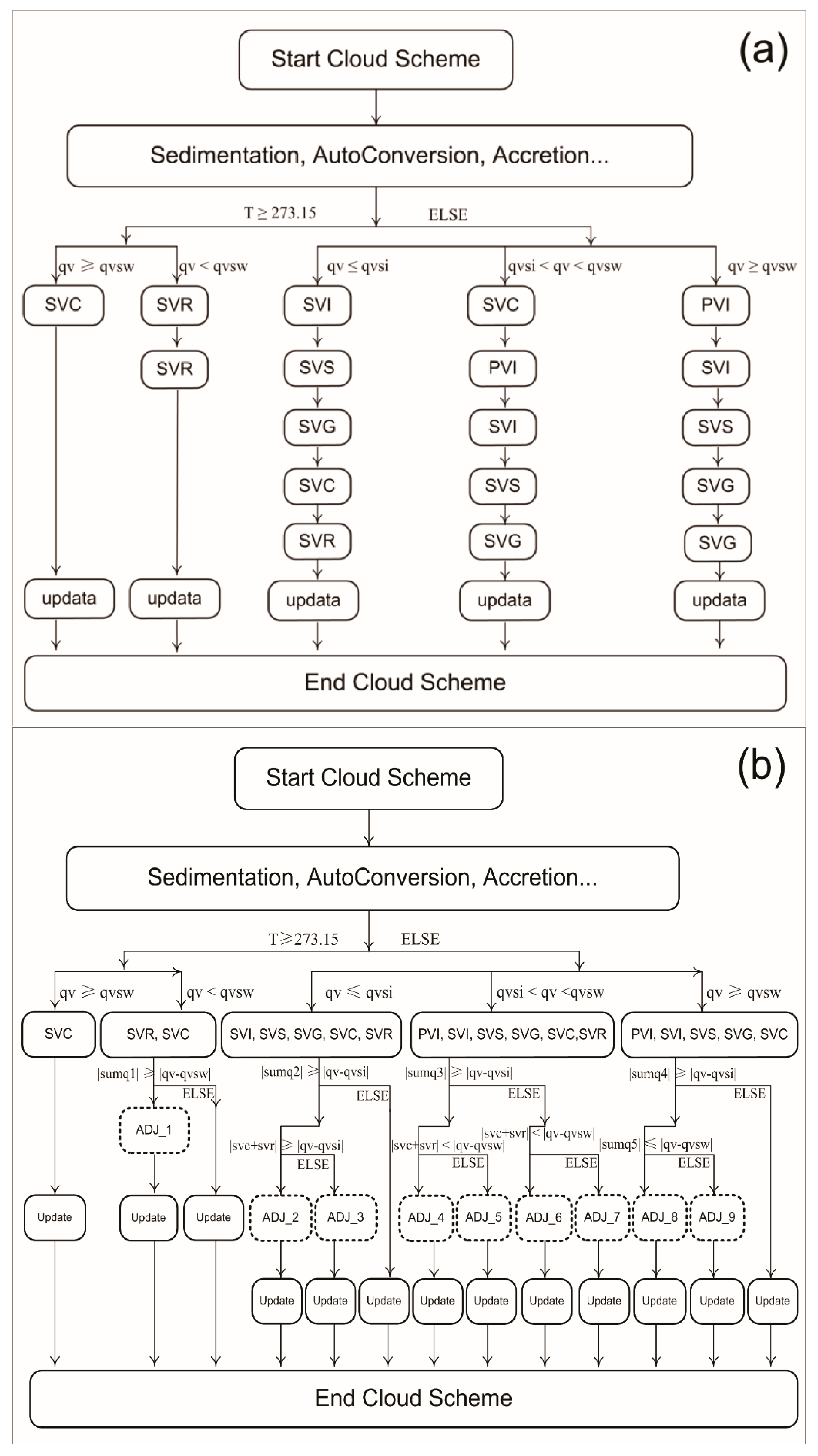
2.2. Descriptions of the SUTA and the PSTA

Detailed descriptions for the two transition approaches are given in this subsection. Figure 1 shows the flow charts of the PSTA and the SUTA, which illustrate the orders of calculating the WVRMPs and updating corresponding tendencies of mass and temperature. In the microphysics scheme, the sedimentation processes of hydrometeors with falling speed are calculated first as well as surface precipitation, and then the conversion processes among different categories of cloud particles are computed. The last part is to compute the WVRMPs, which is what we focus on in this study.

For the SUTA, when the water vapor (${\mathrm{q}}_{\mathrm{v}}$) in the atmosphere is supersaturated with respect to water in the warm region (T ≥ 0 °C), only the condensation rate of cloud droplets ($\mathrm{SVC}$) and its tendency update are calculated. Contrarily, when the water vapor content is subsaturated with respect to water, the evaporation rate of cloud droplets and the update of mass and temperature tendencies are firstly computed, and then those of raindrops are followed. In the cold region (T < 0 °C), these transition processes become complicated because the solid-phase and liquid-phase hydrometeors coexist, and the saturated specific humidity with respect to water is higher than that with respect to ice. When the water vapor content in the environment is less than the saturated specific humidity with respect to ice (${\mathrm{q}}_{\mathrm{vsi}}$), all categories of hydrometeors undergo the sublimation or evaporation process. Therefore, the rates of sublimation or evaporation in order of ice crystals ($\mathrm{SVI}$), snow ($\mathrm{SVS}$), graupels ($\mathrm{SVG}$), cloud droplets ($\mathrm{SVC}$), and raindrops ($\mathrm{SVR}$) are calculated sequentially. After each process, their tendencies of mass and temperature are updated. Similarly, when the air is supersaturated with respect to water (${\mathrm{q}}_{\mathrm{v}}<{\mathrm{q}}_{\mathrm{vsw}}$), water vapor will transit into solid-phase or liquid-phase hydrometeors through the deposition or condensation process. In this condition, the calculations for the transition rates and tendency updates are conducted in order of the initial nucleation of ice crystals ($\mathrm{PVI}$), the deposition of ice crystals ($\mathrm{SVI}$), snow ($\mathrm{SVS}$), and graupels ($\mathrm{SVG}$), and the condensation of cloud droplets ($\mathrm{SVC}$). When water vapor content in the atmosphere is between the saturated specific humidity with respect to ice and that with respect to water, the “Bergeron Process” occurs. That is, the liquid-phase cloud particles undergo the evaporation process, and ice-phase cloud particles undergo the deposition process. In the SUTA, the evaporation of cloud droplets and the tendency update are calculated first, and then the ice crystal initial nucleation, ice-phase deposition processes in order from small to large particles (ice crystals, snow, and graupels) along with tendency update are processed one by one.

A new well physically-based parallel-split transition approach (PSTA) for the WVRMPs is developed in this study, and its flow chart is shown in Figure 1b. For the PSTA, when the air is supersaturated with respect to water in the warm region, the condensation rate of cloud droplets ($\mathrm{SVC}$) is calculated. In contrast, the evaporation processes of cloud droplets ($\mathrm{SVC}$) and raindrops ($\mathrm{SVR}$) are calculated simultaneously with the same humidity and temperature state when the air is subsaturated over a liquid surface. To ensure that the total evaporation rate of $\mathrm{SVC}$ and $\mathrm{SVR}$ does not overshoot the maximum evaporable rate of water vapor ((${\mathrm{q}}_{\mathrm{v}}-{\mathrm{q}}_{\mathrm{vsw}})/\mathrm{dt}$) at the grid in a time step, necessary adjustments for their transition rates need to be carried out. When the total evaporation rate of $\mathrm{SVC}$ and $\mathrm{SVR}$ ($\mathrm{sumq}1$) is less than the maximum evaporable rate of water vapor at the current time step, that is $\mathrm{sumq}1<\left({\mathrm{q}}_{\mathrm{v}}-{\mathrm{q}}_{\mathrm{vsw}}\right)$, their own tendencies of mass and temperature will be updated accordingly. On the contrary, when the sum of $\mathrm{SVC}$ and $\mathrm{SVR}$ is greater than (${\mathrm{q}}_{\mathrm{v}}-{\mathrm{q}}_{\mathrm{sw}})/\mathrm{dt}$, that is $\mathrm{sumq}1\ge \left({\mathrm{q}}_{\mathrm{v}}-{\mathrm{q}}_{\mathrm{vsw}}\right)$, a transition-rate-weighted (TRW) method of $\mathrm{SVC}$ and $\mathrm{SVR}$ is used to allocate the maximum evaporable rate to $\mathrm{SVC}$ and $\mathrm{SVR}$ according to their weights (“Adj_1” in Figure 1b). The mass tendencies of water vapor, cloud droplets, and raindrops and corresponding temperature change caused by the released latent heat are finally updated.

In the cold region, when the air is subsaturated with respect to ice (${\mathrm{q}}_{\mathrm{v}}\le {\mathrm{q}}_{\mathrm{vsi}}$), the evaporation of liquid-phase cloud particles ($\mathrm{SVC}$, $\mathrm{SVR}$) and the sublimation of ice-phase cloud particles ($\mathrm{SVI}$, $\mathrm{SVS}$, $\mathrm{SVG}$) occur simultaneously. Similarly, all the transition processes are calculated with the same environmental state. Thus, the TRW method for each process also is necessary to avoid overshooting the maximum sublimable rate $\left({\mathrm{q}}_{\mathrm{v}}-{\mathrm{q}}_{\mathrm{vsi}}\right)/\mathrm{dt}$ in the time step. In this case, when the total amount of evaporation and sublimation rates ($\mathrm{sumq}2=\mathrm{SVC}+\mathrm{SVR}+\mathrm{SVI}+\mathrm{SVS}+\mathrm{SVG}$) is less than the maximum sublimatable rate $({\mathrm{q}}_{\mathrm{v}}-{\mathrm{q}}_{\mathrm{vsi}})/\mathrm{dt}$, it only needs to update their mass and temperature tendencies without the adjustment. However, when the total evaporation and sublimation rates are greater than the maximum sublimable rate, that is $\mathrm{sumq}2>\left({\mathrm{q}}_{\mathrm{v}}-{\mathrm{q}}_{\mathrm{vsi}}\right)/\mathrm{dt}$, there are two scenarios that may happen. On the one hand, when the total evaporation rate of cloud droplets and raindrops ($\mathrm{SVC}+\mathrm{SVR}$) exceeds the value of $\left({\mathrm{q}}_{\mathrm{v}}-{\mathrm{q}}_{\mathrm{vsi}}\right)/\mathrm{dt}$, the sublimation processes are not considered to occur, and then the adjustments are implemented to allocate the maximum sublimatable rate to $\mathrm{SVC}$ and $\mathrm{SVR}$ according to their transition rate weights. On the other hand, all the evaporation and sublimation processes are considered to occur simultaneously when the sum of $\mathrm{SVC}$ and $\mathrm{SVR}$ is less than the sublimatable rate; thus, the value of $\left({\mathrm{q}}_{\mathrm{v}}-{\mathrm{q}}_{\mathrm{vsi}}\right)/\mathrm{dt}$ is allocated to each transition process using the TRW method. After that, the tendency feedback for each process is calculated.

When the air is supersaturated with respect to water, the condensation of cloud droplets, the initial nucleation of ice crystals, and the depositions of ice crystals, snow, and graupels will occur simultaneously. Likewise, adjustments should be applied to these processes to ensure that the total amount of condensation and deposition rates $\mathrm{sumq}4$ ($\mathrm{sumq}4=\mathrm{SVC}+\mathrm{PVI}+\mathrm{SVI}+\mathrm{SVS}+\mathrm{SVG}$) does not overshoot the value of the maximum condensation rate $\left({\mathrm{q}}_{\mathrm{v}}-{\mathrm{q}}_{\mathrm{vsw}}\right)/\mathrm{dt}$ in this time step. Because the saturated specific humidity over the ice surface is less than that over the water surface, the ice deposition happens more easily than cloud droplet condensation. Therefore, when $\mathrm{sumq}4$ is greater than the value of $\left({\mathrm{q}}_{\mathrm{v}}-{\mathrm{q}}_{\mathrm{vsw}}\right)/\mathrm{dt}$, first make sure whether the total deposition rate of ice-phase cloud particles $\mathrm{sumq}5$ ($\mathrm{sumq}5=\mathrm{PVI}+\mathrm{SVI}+\mathrm{SVS}+\mathrm{SVG}$) exceeds the threshold or not. If the value of $\mathrm{sumq}5$ exceeds the threshold, the TRM method will be applied to allocate the maximum condensation rate $\left({\mathrm{q}}_{\mathrm{v}}-{\mathrm{q}}_{\mathrm{vsw}}\right)/\mathrm{dt}$ to $\mathrm{PVI}$, $\mathrm{SVI}$, $\mathrm{SVS}$, and $\mathrm{SVG}$, and the condensation rate of cloud droplets is set to zero. On the contrary, each deposition rate of ice-phase particles will still be kept; meanwhile, the value after deducting the total ice-phase deposition rate $\mathrm{sumq}5$ from $\left({\mathrm{q}}_{\mathrm{v}}-{\mathrm{q}}_{\mathrm{vsw}}\right)/\mathrm{dt}$ is assigned to the amount of condensation of cloud droplets.

When the water vapor content in the atmosphere is between the saturated specific humidity over the ice surface and that over the water surface, the evaporation of cloud water and the deposition of ice-phase particles will occur simultaneously, which is called the “Bergeron Process”. In the PSTA, when the total deposition rate of the ice-phase particles $\mathrm{sumq}3$ ($\mathrm{sumq}3=\mathrm{PVI}+\mathrm{SVI}+\mathrm{SVS}+\mathrm{SVG}$) is less than the value of $\mathrm{qv}-\mathrm{qvsi}$, it needs to be further consider as to whether the total evaporation rate of the liquid-phase particles ($\mathrm{SVC}+\mathrm{SVR}$) exceeds the maximum evaporable rate with the value of $\left(\mathrm{qv}-\mathrm{qvsw}\right)/\mathrm{dt}$ or not. When the value of $\mathrm{SVC}+\mathrm{SVR}$ exceeds the threshold, the value of $\left(\mathrm{qv}-\mathrm{qvsw}\right)/\mathrm{dt}$ will be allocated to $\mathrm{SVC}$ and $\mathrm{SVR}$ according to their transition rate weights. In other cases, the evaporation/deposition rates of all categories of cloud particles remain unchanged. When the total condensation of ice-phase particles $\mathrm{sumq}3$ is greater than the value of $\left(\mathrm{qv}-\mathrm{qvsi}\right)/\mathrm{dt}$, the TRW method is adopted to allocate the maximum depositable amount to each transition of $\mathrm{PVI}$, $\mathrm{SVI}$, $\mathrm{SVS}$, and $\mathrm{SVG}$. Meanwhile, the value of $\left(\mathrm{qv}-\mathrm{qvsw}\right)/\mathrm{dt}$ is used as the threshold value to determine whether to adjust the evaporation rates of cloud droplets and raindrops or not. Note that here we only consider the coexistence of the evaporation process and deposition process of different phase cloud particles calculated with the same temperature and humidity state and do not really consider the triple-phase transformations of water substance involved in the “Bergeron Process”. Because the “Bergeron process” is a dynamic transition process, the first calculation process will inevitably bring about changes in temperature and humidity, which further change the ambient conditions of the subsequent calculation process; thus, the whole process will become very complicated. In addition, since the integration time step (30 s) is relatively short, the effects of the Bergeron process on clouds and precipitation within a time step can be ignored. Actually, the Bergeron process is rarely treated specially in the codes of most current microphysics schemes.

3. Model and Dataset

3.1. CMA_MESO Model

Since the 2000s, the China Meteorological Administration (CMA) has been devoted to building its own NWP system based on the Global/Regional Assimilation and Prediction System (GRAPES). Up to now, a suite of complete numerical forecasting systems at the CMA, including global medium-range, regional, ensemble, and typhoon simulations, has been established with steadily improved prediction performance [29,30,31,32,33]. Among them, the GRAPES regional 3-km high-resolution deterministic prediction system, renamed the CMA-MESO model in 2021, covering the whole of China, became operational in June 2018. Version 5.0 of the CMA-MESO operational system is employed in this study. The dynamical core of the CMA-MESO v5.0 and its physical parameterization schemes have been introduced in Ma et al. [13], and we will not repeat them here.

3.2. Experiment Setup

A heavy rainfall case that occurred in central China on 23 June 2017 was simulated for a detailed analysis of the influences of the STUA and PSTA on hydrometeors, transition rates, latent heat, and surface precipitation. In addition, batch experiments for simulating the summer precipitation in 2017 were carried out to analyze further the impact on QPFs. The analysis and forecast fields of the National Centers for Environmental Predication Global Forecast System (NCEP/GFS) were treated for the initial conditions and time-varying lateral boundary conditions at 6-h intervals. All of the simulations were run at a 0.03° horizontal grid spacing resolution with 561 × 931 grid points in the south-north and east-west directions, respectively. There were 50 vertical stretched sigma levels from the surface up to the model top at 10 hPa. All of the simulations were integrated for 48 h with a time step of 30 s. The simulation domain covered South China, which is shown in Figure 2. The double-moment cloud microphysics scheme with the SUTA and PSTA options described above, referred to as the SUTA experiment and PSTA experiment, respectively, was employed in this study. Except for the cloud microphysics scheme, the other physical schemes used in this experiment were consistent with the operational application, which were the RRTM long-wave radiation scheme [34], the Dudhia short-wave radiation scheme [35], the Noah land surface scheme [36], and the NMRF planetary boundary layer scheme [37]. The cumulus convection scheme was not used since the horizontal resolution reaches the cloud-resolving scale in this study.

3.3. Gauge Precipitation

To quantitatively validate the daily amount of precipitation simulated by the two transition approaches in the double-moment microphysics scheme, a daily accumulated precipitation database from the CMA precipitation gauge network was employed in this study. The precipitation datasets are widely used in research, as applied by Su et al. [38]. There are a total of 1236 gauges in the simulation domain, as shown in Figure 2.

4. Results

4.1. Analysis of Rainfall Event

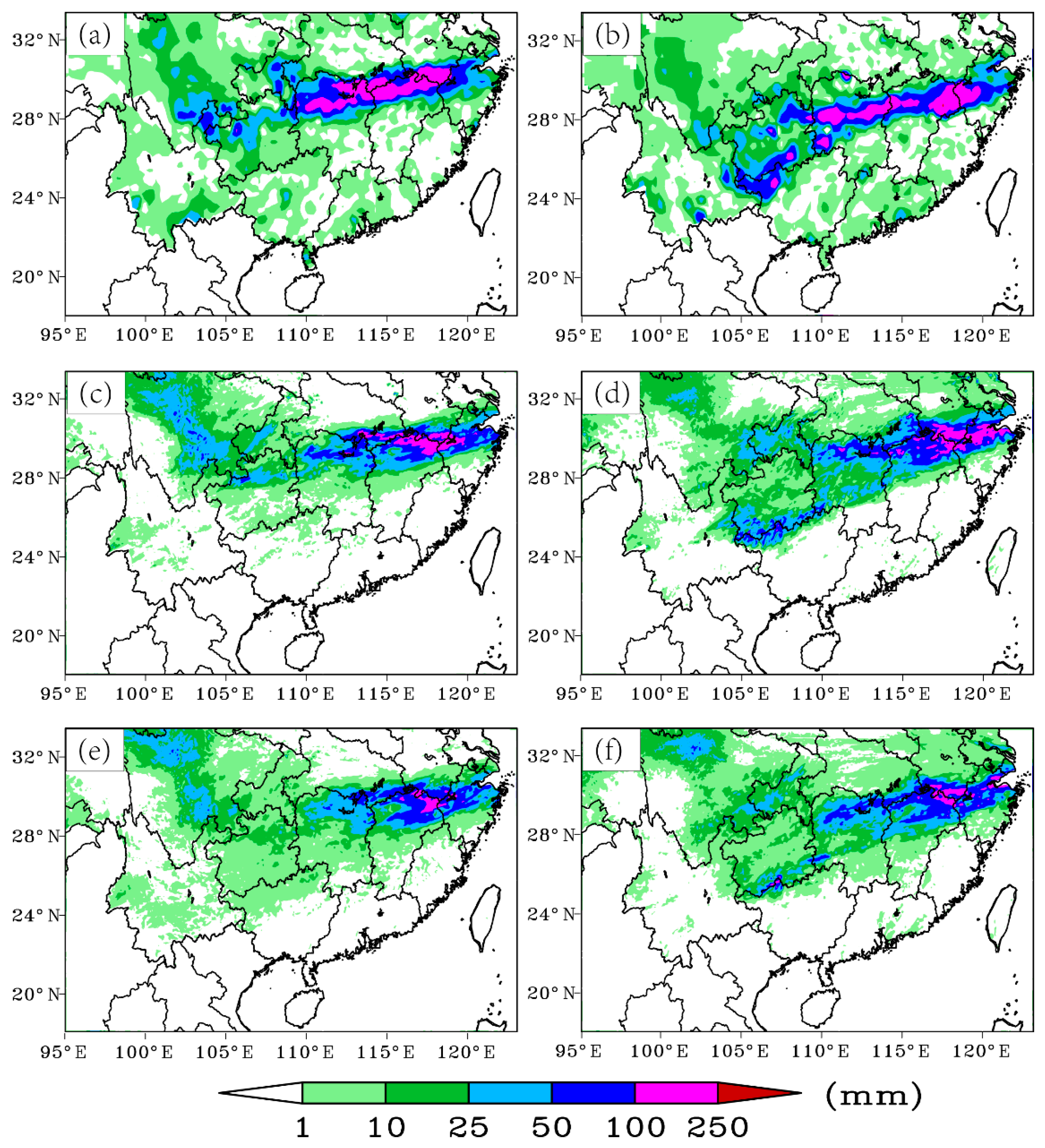
4.1.1. Precipitation

To analyze the impacts of the transition approach of the WVRMPs on the QPFs, a mesoscale convective system (MCS) case, which occurred over central China from 23 June to 25 June 2017, was simulated. Figure 3 shows the simulated 24-h and 48-h accumulated precipitation and gauge observations. As shown in Figure 3a, the observed 24-h precipitation belt is located within the range of 102° E–121° E and 26° N–30° N, oriented from southwest to northeast. According to the meteorological observation standard of the CMA, rainfall events with 24-h accumulated precipitation of 0.1–9.9 mm, 10.0–24.9 mm, 25–49.9 mm, 50.0–99.9 mm, 100.0–249.9 mm, and over 250.0 mm are defined as light rainfall, moderate rainfall, heavy rainfall, torrential rainfall, rainstorm, and heavy rainstorm, respectively, which has also been adopted by Su et al. [38]. The high-value precipitation areas with torrential rainfall or more (>50 mm) are concentrated in the domain of 110° E–120° E and 28° N–30° N, where there is a total of 35 stations with rainstorms (100–249.9 mm). Generally, the SUTA experiment and the PSTA experiment both well simulate the location and distribution range of the precipitation case (Figure 3c,e). Although the two experiments both underestimate the torrential rainfall and the rainstorm over the main rain belt areas to some extent, the PSTA experiment has advantages over the SUTA experiment in precipitation magnitude. The PSTA experiment simulates a narrower distribution range with a high magnitude for 24-h accumulative precipitation compared with that of the the SUTA experiment, which is closer to the observed precipitation. For example, it is clear that more torrential rainfall and rainstorm consistent with observations occurred in the PSTA experiment over the main rain belt area (110° E–120° E, 28° N–30° N), while the precipitation above the magnitude of 100 mm (rainstorm) is significantly underestimated in the SUTA experiment.

Similarly, the characteristics and differences of the 48-h precipitation simulations in the two experiments are similar to those of the 24-h precipitation simulation compared with the observed precipitation. The distribution range of the rain belt and its precipitation amount in the PSTA experiment is more consistent with the observations. The above-simulated precipitation differences are directly related to the two transition approaches, which will be explained in detail in Section 4.1.2.

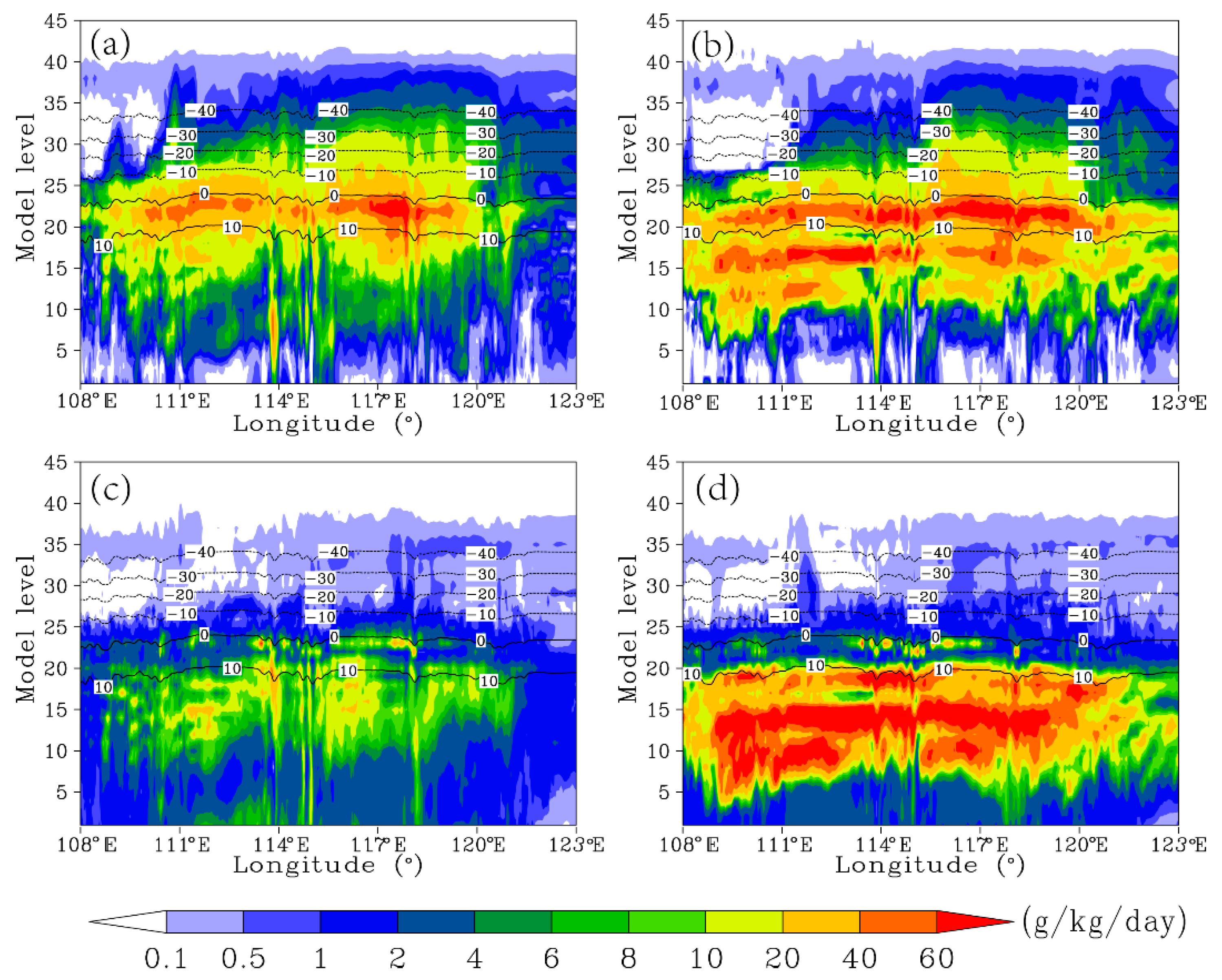
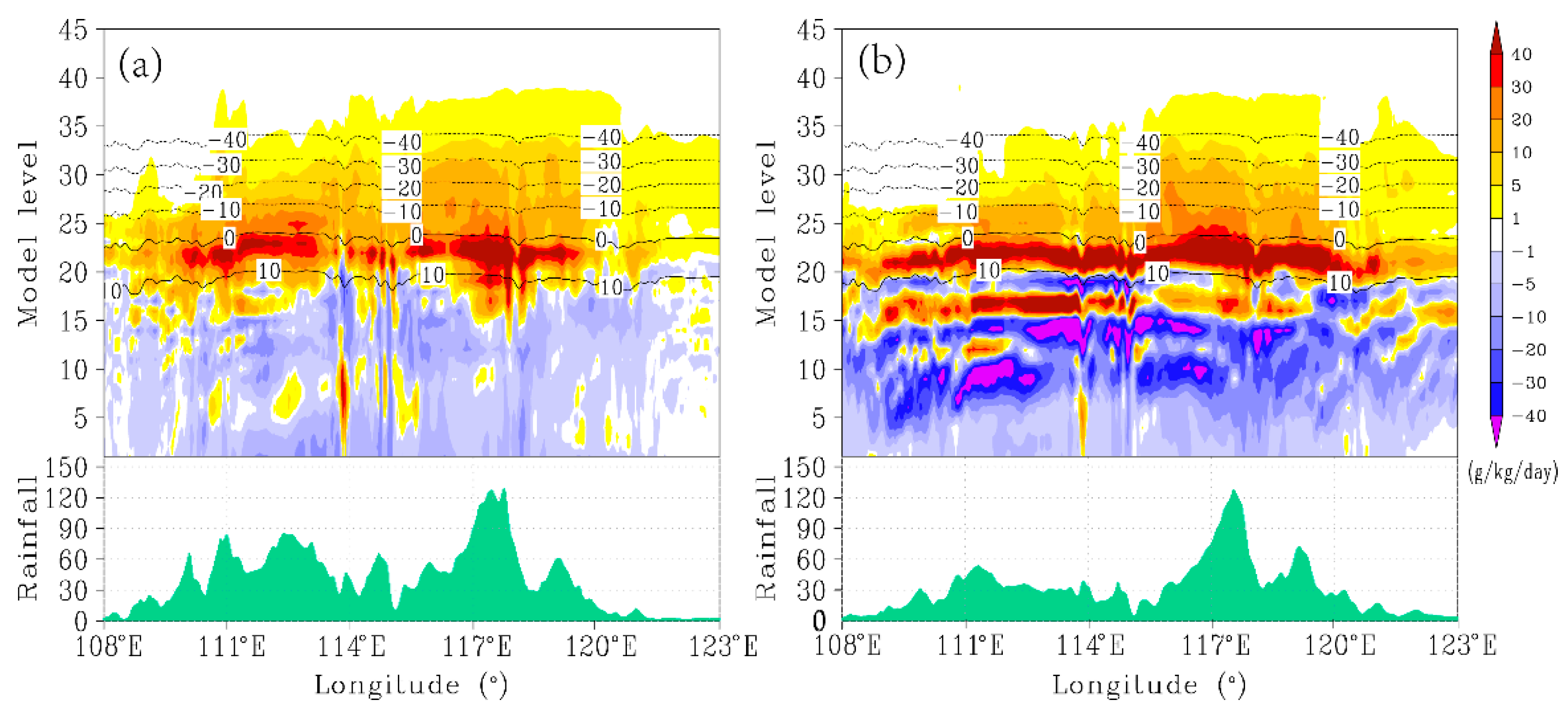
4.1.2. Source and Sink Terms of WVRMPs

In this subsection, the characteristics of the transition rates and their differences for the WVRMPs simulated by the SUTA and PSTA are investigated to analyze their impacts on the formation and dissipation of clouds and surface-precipitation forecasting. Figure 4 shows the vertical latitude cross-sections of the 24-h-averaged total condensation/deposition rate and total evaporation/sublimation rate from the two experiments along the central location of this precipitation case (the latitude of 29.5° N). As seen, for both the total condensation/deposition rate and total evaporation/sublimation rate, their values simulated by the PSTA are systematically smaller with more gentle changes than those from the SUTA experiment in the warm region ($\mathrm{T}\ge 0°\mathrm{C}$); however, their differences are not significant in the cold region ($\mathrm{T}<0°\mathrm{C}$). Taking the total condensation/deposition rate as an example, the region with values exceeding 20 g kg⁻¹ d⁻¹ simulated by the PSTA is mainly distributed between layer 15 and layer 25, while the region with the responding values simulated by the SUTA is mainly between layer 10 and layer 25. Moreover, the area with a high condensation/deposition rate (above 40 g kg⁻¹ d⁻¹) in the PSTA experiment is obviously smaller than that in the SUTA experiment. It is worth noting that, overall, the total condensation/deposition rate in the ice–liquid mixing areas from the PSTA experiment is slightly greater than that from the SUTA experiment, such as at the heights with temperatures between −20 °C and 0 °C. For the total evaporation rate of the PSTA experiment, it is evident that there is a weak evaporation process in warm regions, where its values are mostly below 20 g kg⁻¹ d⁻¹. In the corresponding regions, most of the total evaporation rates from the SUTA experiment are above 20 g kg⁻¹ d⁻¹, indicating that the SUTA scheme is prone to lead to more evaporation processes of cloud water and rainwater. In the cold region, the total evaporation/sublimation rate of the PSTA experiment is slightly larger than that of the SUTA experiment, which has a wider distribution with values above 1 g kg⁻¹ d⁻¹.

To reveal the integral (combined) effects of the two transition approaches on QPF, their simulated net transition rate between water vapor and hydrometeors, that is, the total transition rate of all the WVRMPs (SVC + SVR + PVI + SVI + SVS + SVG), and the corresponding 24-h accumulated precipitation along the precipitation center (the latitude of 29.5° N) are plotted, as shown in Figure 5. As seen, the WVRMPs from the two experiments are both dominated by the cloud formation process (net condensation/deposition) in the middle and upper model layers (from layer 18 to layer 37) and are dominated by the cloud dissipation process (net evaporation) below the cloud base, which conforms to the natural characteristics of clouds. However, their values of net transition rate are different. Similar to the results of total condensation/deposition and total evaporation/sublimation, the net transition rate simulated by the PSTA presents a more continuous and steadier distribution with smaller values compared with those of the SUTA, while the net transition rate simulated by SUTA is characterized by large values and violent fluctuations in the warm region. For example, there is greater net condensation (deposition) amounts at the heights with temperatures of 0 °C–10 °C (layer 18 to layer 23) in the simulation by the SUTA than the PSTA, indicating that more cloud droplets are condensed. Meanwhile, apparent fluctuations in the net transition rate from the SUTA experiment occur at the heights below layer 18. For the PSTA experiment, it simulates the net transition rate with the values mostly between 10 g kg⁻¹ d⁻¹ and 30 g kg⁻¹ d⁻¹ and locally up to 40 g kg⁻¹ d⁻¹ at the height with temperatures of 0 °C–10 °C. The junction areas between the net condensation and net evaporation are smoother and more natural in the warm region compared with the SUTA. The net evaporation rate simulated by the PSTA below the cloud base is obviously smaller than that simulated by the SUTA. The net evaporation rate simulated by the PSTA is below −10 g kg⁻¹ d⁻¹ in most areas, reaching the value of −20 g kg⁻¹ d⁻¹ locally. However, the net evaporation simulated by the SUTA is significantly stronger between layer 5 and layer 15, with the values ranging from −20 g kg⁻¹ d⁻¹ to −40 g kg⁻¹ d⁻¹ and even greater locally. In the cold region, the net condensation/deposition rate in the PSTA experiment is slightly greater than that in the SUTA experiment, but their difference is not significant.

The surface precipitation amount is affected by the net transition rate between water vapor and hydrometeors. The net transition rate in the SUTA experiment is greater than that of the PSTA experiment, especially at the height between 0 °C and 10 °C. However, accompanied by more intense evaporation processes below the cloud base in the SUTA simulation, its surface precipitation amount is less than that of the PSTA, which is the same result as the difference between 24 h and 48 h surface accumulative precipitation (Figure 3). For the PSTA experiment, as shown in Figure 5a, it simulates more surface precipitation compared with the SUTA experiment in most of the region west of 118° E since its corresponding net evaporation rate below the cloud base is less than that of the SUTA. For instance, the precipitation values near 110° E simulated by the SUTA and the PSTA are 53 mm and 85 mm, respectively. At this location, the net evaporation simulated by the SUTA is over −40 g kg⁻¹ d⁻¹, while that by the PSTA is only about −10 g kg⁻¹ d⁻¹. To the east of 118° E, the precipitation simulated by the SUTA is slightly more than that by the PSTA, which is related to more condensation (deposition) in clouds and relatively less evaporation below the cloud base.

The 24-h averaged vertical profiles of the tendencies of each of the WVRMPs and their net tendencies between water vapor and cloud particles over the heavy rainfall region (108° E–120° E, 27.5° N–30° N) are analyzed to reveal their differences simulated by the two transition approaches, which are shown in Figure 6. Both the PSTA and the SUTA well simulate the vertical distributions of conversion between ice-phase hydrometeors and water vapor in the cold regions, but the amounts of conversion rates simulated by the PSTA are higher than those simulated by the SUTA. For example, the deposition process of ice crystals in the two simulations occurs in a deep range, from layer 22 to layer 43 of the model, while the depositions of snows and graupels are mainly distributed in the middle and lower layers of the cold region. In the simulation by the PSTA, the 24-h averaged deposition rates of ice crystal (C_SVI), snow (C_SVS), and graupel (C_SVG) are 1.22 g kg⁻¹ d⁻¹, 1.10 g kg⁻¹ d⁻¹, and 1.01 g kg⁻¹ d⁻¹, respectively. In addition, the corresponding transition rates simulated by the SUTA are slightly smaller, with the values of 1.07 g kg⁻¹ d⁻¹, 1.06 g kg⁻¹ d⁻¹, and 0.76 g kg⁻¹ d⁻¹, respectively. The sublimation process of ice phase particles in the cold region is weaker than the deposition process, and the transition rates simulated by the PSTA are also slightly stronger than that by the SUTA. The average sublimation amount of ice crystals (E_SVI), snow (E_SVS), and graupel (E_SVG) simulated by the PSTA are 0.109 g kg⁻¹ d⁻¹, 0.266 g kg⁻¹ d⁻¹, and 0.15 g kg⁻¹ d⁻¹, respectively. Those simulated by SUTA have values that are 0.09 g kg⁻¹ d⁻¹, 0.23 g kg⁻¹ d⁻¹, and 0.097 g kg⁻¹ d⁻¹, respectively. The initial nucleation of ice crystals (C_PVI) simulated by the two transition approaches are the weakest among all the ice-phase processes, and the C_PVI values simulated by the PSTA and SUTA are 0.089 g kg⁻¹ d⁻¹ and 0.018 g kg⁻¹ d⁻¹, respectively. For the difference in the conversion rates between the ice-phase hydrometeor and water vapor simulated by the two transition approaches, the main reasons are as follows. At each integration step of the model, the same initial value of water vapor is used to calculate the conversion rate of ice-phase particles in the PSTA simulation. When the water vapor reaches supersaturated, compared with the SUTA, the deposition simulated by the PSTA tends to deplete more water vapor and produce more ice-phase hydrometeors.

For the warm cloud microphysics process, both the condensation of cloud water (C_SVC) and the evaporation of cloud water (E_SVC) and rainwater (E_SVR) simulated by the PSTA are steadier and smaller than those simulated by the SUTA. The condensation process of cloud water is taken as an example. The maximum value simulated by the SUTA is 50.3 g kg⁻¹ d⁻¹, and its average value is 11 g kg⁻¹ d⁻¹, while the corresponding values simulated by the PSTA are 31.5 g kg⁻¹ d⁻¹ and 6 g kg⁻¹ d⁻¹, respectively. Moreover, the transition rate simulated by the SUTA varies greatly between layer 14 and layer 20, with more violent distributions. For the evaporation processes of cloud water and rainwater, the same characteristics are also shown.

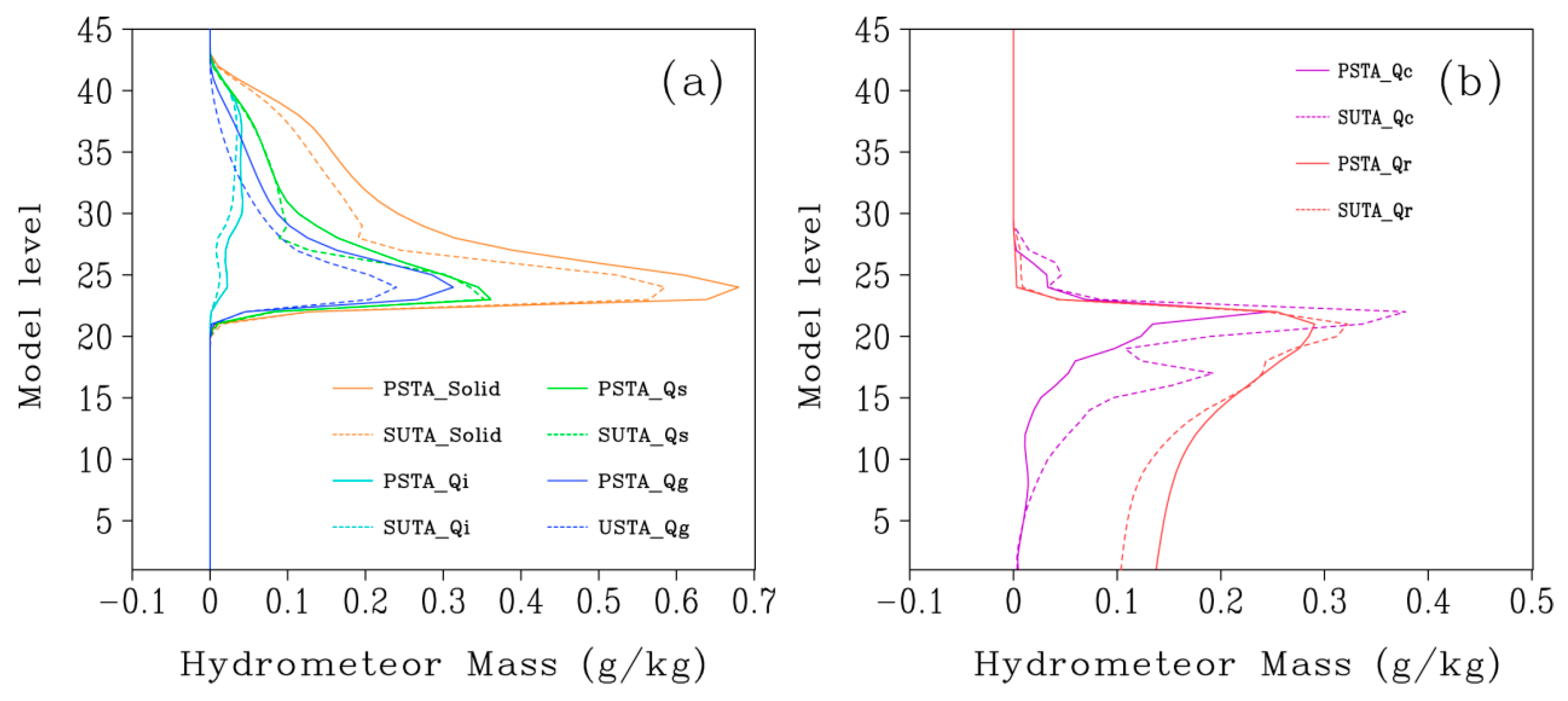
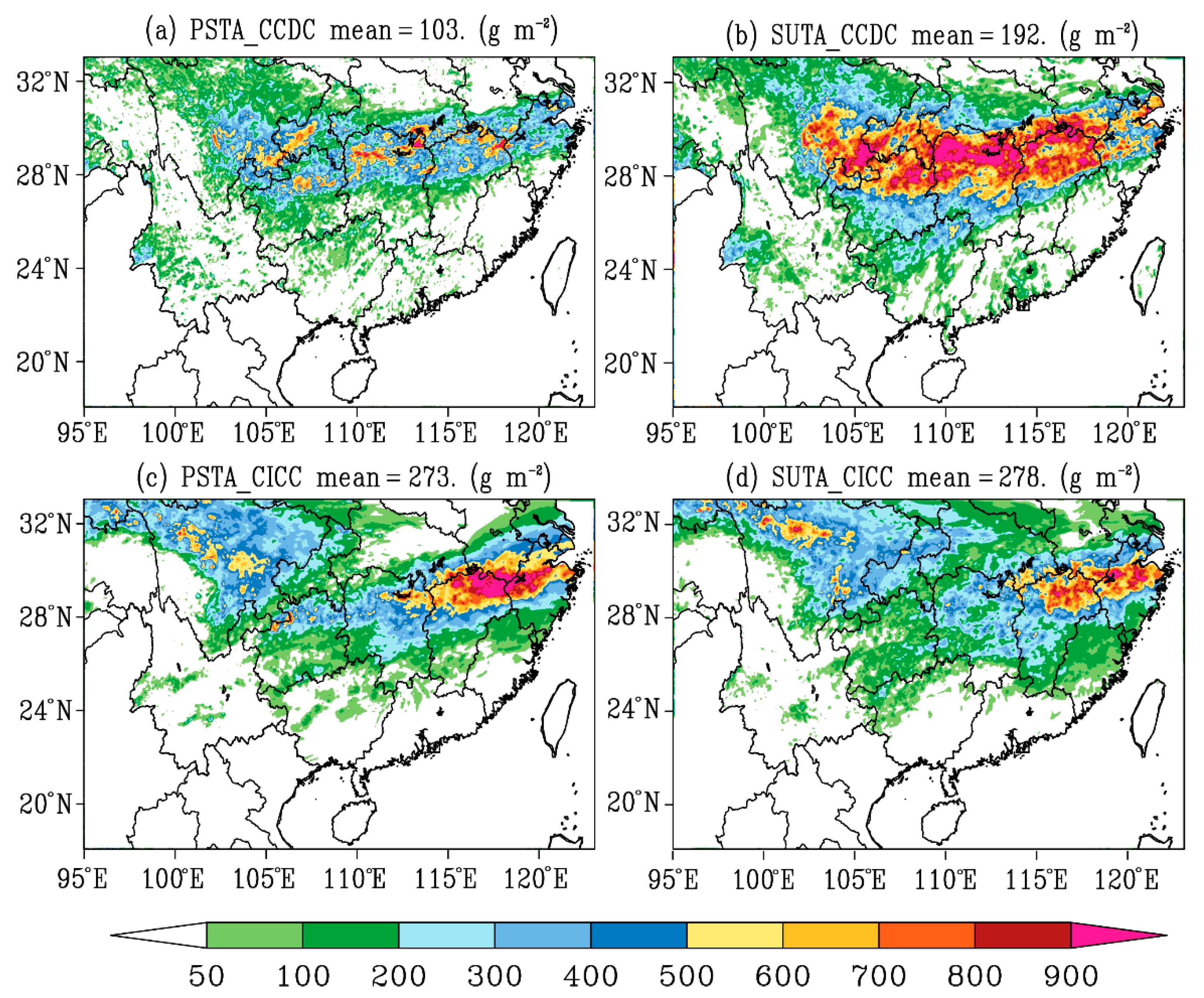
4.1.3. Hydrometeor Contents

The precipitation in the microphysics scheme comes from the sedimentation of different categories of hydrometeor, so the precipitation amount on the ground is directly determined by the mass contents of all cloud particles falling in the atmosphere. In this subsection, the vertical distributions of the hydrometeors simulated by the two transition approaches are analyzed, which are shown in Figure 7. It can be seen that the vertical distribution structures of the ice-phase hydrometeors in the two experiments are very consistent, yet there are systematic differences in their mass content. The PSTA tends to simulate more ice-phase cloud particles than the SUTA in cold regions (Figure 7a). The mass difference of graupel between the two experiments is the most significant among all the ice-phase hydrometeors, which has a difference of 0.09 g kg⁻¹ at the height of the 24th layer. At heights between layers 22 and 40, the PUSA simulated slightly larger ice water content than the SUTA, with a range of less than 0.2 g kg⁻¹. The differences in snow mass content are distributed in a relatively shallow range between 25 and 32 layers, with a maximum difference of 0.07 g kg⁻¹. Apparently, there are more total ice-phase contents in the PSTA simulation compared with the SUTA simulation, and their maximum values are 0.67 g kg⁻¹ and 0.56 g kg⁻¹, respectively. The largest difference occurred at the height of the 28th layer, reaching 0.16 g kg⁻¹.

However, in contrast to ice-phase hydrometeors, it can be found in Figure 7b that the PSTA simulates less liquid-phase cloud particles than the SUTA in almost all warm regions and mixing-phase regions since it has weaker evaporation processes of cloud droplets and raindrops. Similar to the vertical distributions of transition tendency shown in Figure 6, the profiles of liquid-phase hydrometeors simulated by the PSTA are smoother with smaller values compared with those of the SUTA experiment. The profile of cloud droplets in the SUTA simulation has remarkable fluctuations between layers 15 and 23, with a maximum value of 0.37 g kg⁻¹, greater than the 0.25 g kg⁻¹ of the PSTA. Below the cloud base (about 15th layer), the PSTA considerably has more raindrop content than the SUTA due to the weak evaporation process, which makes the central precipitation amount in the PSTA simulation greater than the SUTA (Figure 3).

Column integrated mass content indicates the total content of each hydrometeor in the atmosphere. The horizontal distributions of 24-h averaged column cloud droplet content (CCDC), and the column ice crystal content (CICC) are plotted in Figure 8. The CCDC simulated by the PSTA is obviously less than that of the SUTA experiment, which is the same as the results revealed in Figure 7. Over the main precipitation belt (22° N–30° N and 98° E–122° E), the CCDC with the averaged value of 103 g m⁻² in the PSTA simulation is mostly under 500 g m⁻². Yet, for the SUTA experiment, the simulated 24-h averaged CCDC values are mostly above 500 g m⁻² over the heavy rainfall areas (>50 mm d⁻¹). Its averaged CCDC is up to 192 g m⁻², which is about 1.86 times that simulated by PSTA. Although the SUTA simulates more cloud droplet content compared to PSTA, the violent evaporation process of raindrops in the warm region means that it has little contribution to the surface precipitation amount (Figure 6b). Similar to their simulated precipitation distributions and magnitudes, the PSTA tends to produce more CICCs with more concentrated distributions over the precipitation belt. Although the mean values of CICC simulated by the two transition approaches are very close (273 g m⁻² and 278 g m⁻² for the PSTA and SUTA, respectively), there are great differences in their distribution range and central intensity. For example, the maximum value of the PSTA can reach above 1800 g m⁻² locally in this case, greater than that of the SUTA (1400 g m⁻²).

4.2. Assessment of Batch Experiments

Batch experiments for precipitation simulation from June to August 2017 were carried out to evaluate the influence of the two transition approaches objectively, using QPFs in CMA-MESO v5.0. The average precipitation amount and equitable threat score (ETS) [39] are analyzed below.

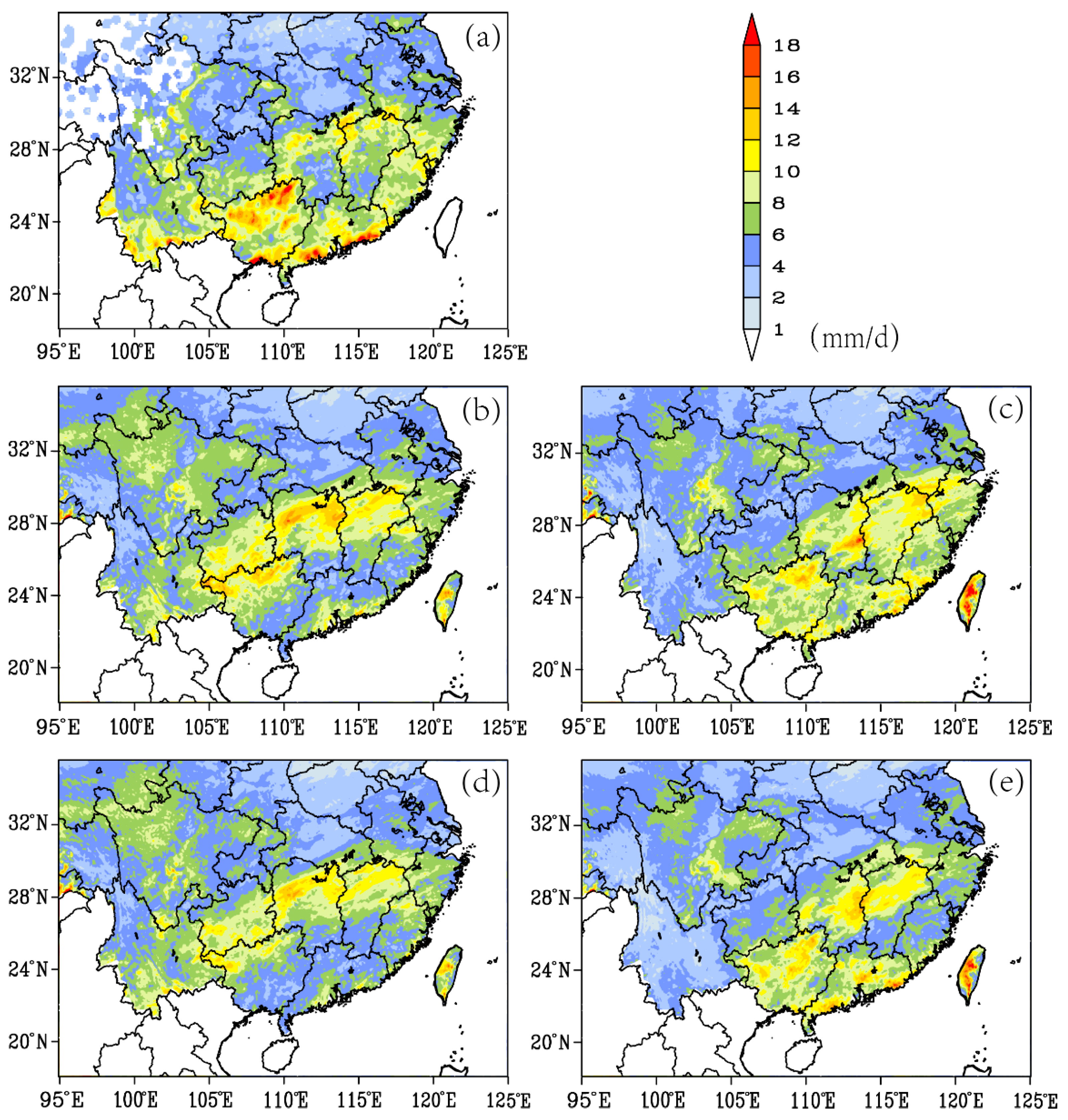
4.2.1. Average Precipitation Amount

Figure 9 shows the distributions of observed and simulated average precipitation amounts for the summer (from June to August) in 2017. In the simulation domain, most of the observed precipitation is above 2 mm d⁻¹, and the precipitation with values greater than 6 mm d⁻¹ is mainly distributed in the south of 29° N, locally reaching 18 mm d⁻¹. Both the two transition approaches well simulate the southwest–northeast rain belt located in the domain of 98° E–122° E and 22° N–29° N, where their average precipitation amounts and rainfall belt distributions are close to the observations. Generally, the precipitation intensity simulated by the PSTA is slightly greater than that of the SUTA over the above areas (Figure 9b,d). In addition, although the PSTA-simulated precipitation amount is somewhat superior to the SUTA in this region, with a certain increase in precipitation amount, they still have the common phenomenon of underestimating precipitation in warm sectors along the south coastline areas, which is one of the challenging issues for QPFs in current NWP models. It is evident that the 48-h averaged precipitation amounts simulated by the two transition approaches are both more compared with those of 24-h simulation, possibly due to the fact that they do not need to go through the spin-up process at the beginning of the integration. Similar to 24-h precipitation, the PSTA simulates a more-averaged precipitation amount for 48-h than the SUTA (Figure 9c,e); for example, there is a broader distribution of precipitation above 6 mm d⁻¹ in the PSTA experiment.

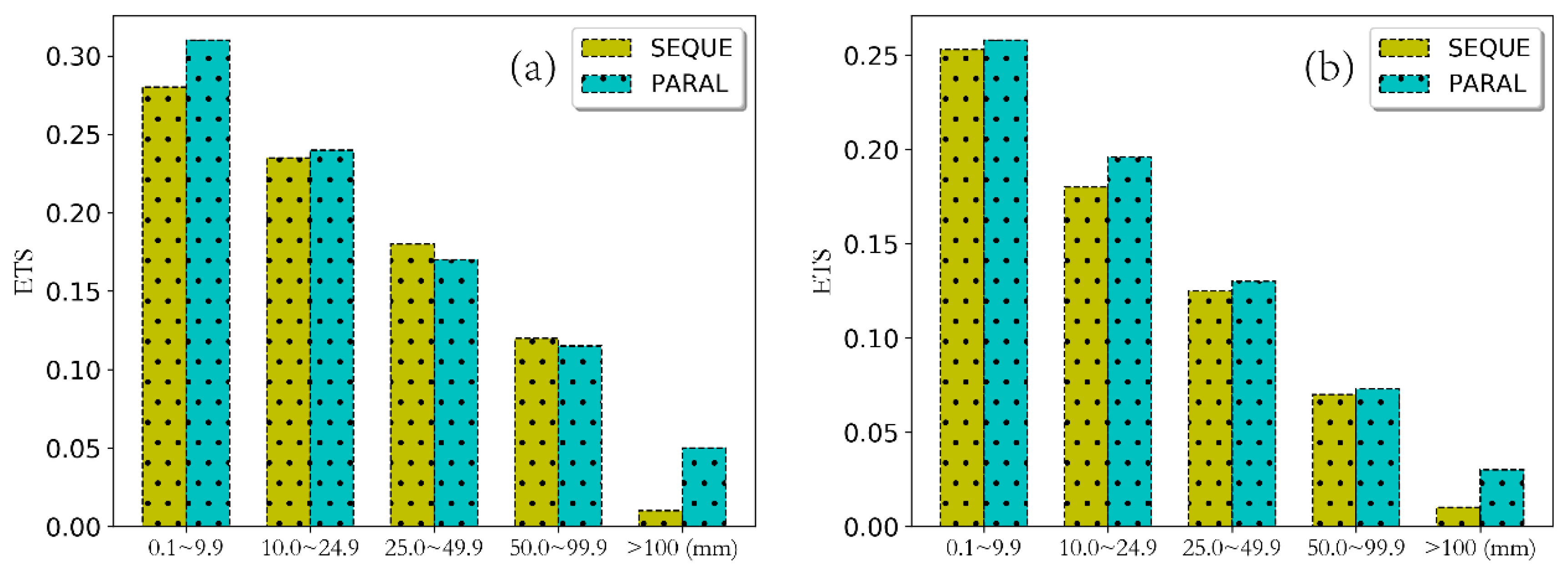
4.2.2. Equitable Threat Score of Precipitation

The ETS is often used for the verification of precipitation forecasts since it measures the skill of a forecast relative to chance. The ETSs of precipitation simulations in different lead times for the summer of 2017 are given in Figure 10. Compared with the SUTA, the ETSs of 24-h precipitation from the PSTA simulation show a neutral and slightly positive effect as a whole. The ETSs of heavy rainfall and torrential rainfall simulated by the PSTA are lower than those simulated by the SUTA, but the ETSs of light rainfall, moderate rainfall, and rainstorm simulated by the PSTA are greater than those from the USTA simulations. In particular, the light rain and rainstorm improved significantly, with the ETSs increasing from 0.28 to 0.31 and from 0.013 to 0.048, respectively. For the 48-h simulations, the PSTA has significant advantages over the SUTA in the performance of precipitation forecasting (Figure 10b). Obviously, the ETSs for all magnitudes of precipitation simulated by the PSTA experiment are improved against the SUTA experiment, especially for moderate rainfall and rainstorm. Therefore, comprehensively, the PSTA has a better performance in precipitation forecasting compared with the SUTA, especially for the 48-h simulations. The above results reveal that reasonable treatments of the WVRMPs would effectively improve the QPFs in the development or optimization of cloud microphysics schemes.

5. Conclusions and Discussion

With the improvement in the horizontal resolution of the numerical weather forecast models, more detailed descriptions of microphysical processes in cloud schemes are important to the QPFs. In this study, a newly developed parallel-split transition approach (PSTA) is applied to the WVRMPs and compared with the original sequential-update transition approach (SUTA) in the double-moment cloud microphysical scheme. Based on the CMA-MESO 3-km operational model, the main characteristics and possible reasons for the impacts of the two transition approaches on cloud and precipitation forecasting are investigated. The main conclusions are as follows.

A new well physically-based parallel-split transition approach (PSTA) to calculate the MPRWVs is applied to the double-moment cloud microphysics scheme at CMA. The PSTA considers different temperature and humidity environments, the difference of the saturated specific humidity over water and ice, and the degree of difficulty in the formation and dissipation of different categories of hydrometeors.

A heavy precipitation case is used to evaluate the performance of the PSTA and SUTA. Compared with the SUTA, the precipitation simulated by the PSTA is closer to the observations, and the PSTA simulates narrower and more concentrated precipitation distributions with a stronger intensity in its precipitation center.

For the processes of condensation (deposition) and evaporation (sublimation), the conversion process is steadier, and their values are smaller in the simulation by the PSTA. In the cold region, the PSTA simulates a net condensation (deposition) process with a higher conversion rate than that simulated by the SUTA, which is not rather significant. In the warm region, the condensation and evaporation processes in the PSTA simulation are significantly weaker than those in the SUTA simulation. The PSTA has more steady evaporation processes below the cloud base with more sedimentary hydrometeors to produce more precipitation.

The verification of the precipitation in the batch experiments shows that the horizontal distribution of precipitation simulated by the PSTA is more reasonable than that simulated by the SUTA, especially the 48-h precipitation, which is closer to the observation. The 24-h precipitation simulated by the PSTA has similar but slightly better ETSs compared with that from the SUTA experiments, and the ETS for the 48-h precipitation from the PSTA experiments has an evident advantage over that of the SUTA experiments for all precipitation magnitudes.

To summarize, this study develops a new, well physical parallel-split transition approach to process the WVRMPs. It can significantly improve the quantitative precipitation forecast in the CMA-MESO 3-km regional model. However, it should be noted that this study only focuses on a summer precipitation analysis and assessment. The net condensation (deposition) rates for the two transition approaches are different in the cold region. In winter, the impacts of the PSTA on snowfall forecasting and whether the result would be consistent with the summer precipitation are still unknown. Further studies need to be conducted in the future.

References

1. Yu, R.C.; Zhang, Y.; Wang, J.J.; Li, J.; Chen, H.M.; Gong, J.D.; Chen, J. Recent Progress in Numerical Atmospheric Modeling in China. Adv. Atmos. Sci. 2019, 36, 938–960. [Google Scholar] [CrossRef]
2. Barszcz, A.; Milbrandt, J.A.; Thériault, J.M. Improving the Explicit Prediction of Freezing Rain in a Kilometer-Scale Numerical Weather Prediction Model. Wea. Forecast. 2018, 33, 767–782. [Google Scholar] [CrossRef]
3. Klein, S.A.; Jakob, C. Validation and Sensitivities of Frontal Clouds Simulated by the ECMWF Model. Mon. Weather Rev. 1999, 127, 2514–2531. [Google Scholar] [CrossRef]
4. Wang, Y.; Fan, J.; Zhang, R.; Leung, L.R.; Franklin, C. Improving bulk microphysics parameterizations in simulations of aerosol effects. J. Geophys. Res. Atmos. 2013, 118, 5361–5379. [Google Scholar] [CrossRef]
5. Milbrandt, J.A.; Morrison, H. Parameterization of Cloud Microphysics Based on the Prediction of Bulk Ice Particles Properties. Part III: Introduction of Multiple Free Categories. J. Atmos. Sci. 2016, 73, 975–995. [Google Scholar] [CrossRef]
6. Thompson, G.; Eidhammer, T. A Study of Aerosol Impacts on Clouds and Precipitation Development in a Large Winter Cyclone. J. Atmos. Sci. 2014, 71, 3636–3658. [Google Scholar] [CrossRef]
7. Morrison, H.; Thompson, G.; Tatarskii, V. Impact of cloud microphysics on the development of trailing stratiform precipitation in a simulated squall line: Comparison of one- and two-moment schemes. Mon. Weather Rev. 2009, 137, 991–1007. [Google Scholar] [CrossRef] [Green Version]
8. Hong, S.-Y.; Dudhia, J.; Chen, S.-H. A Revised Approach to Ice Microphysical Processes for the Bulk Parameterization of Clouds and Precipitation. Mon. Weather Rev. 2004, 132, 103–120. [Google Scholar] [CrossRef]
9. Khain, A.P.; Rosenfeld, D.; Pokrovsky, A. Aerosol impact on the dynamics and microphysics of deep convective clouds. Quart. J. R. Meteor. Soc. 2005, 131, 2639–2663. [Google Scholar] [CrossRef] [Green Version]
10. Flossmann, A.I.; Wobrock, W. A review of our understanding of the aerosol—Cloud interaction from the perspective of a bin resolved cloud scale modelling. Atmos. Res. 2010, 97, 478–497. [Google Scholar] [CrossRef]
11. Vié, B.; Pinty, J.P.; Berthet, S.; Leriche, M. LIMA (v1.0): A quasi two-moment microphysical scheme driven by a multimodal population of cloud condensation and ice freezing nuclei. Geosci. Model Dev. 2016, 9, 567–586. [Google Scholar] [CrossRef] [Green Version]
12. Morrison, H.; Grabowski, W.W. A Novel Approach for Representing Ice Microphysics in Models: Description and Tests Using a Kinematic Framework. J. Atmos. Sci. 2008, 65, 1528–1548. [Google Scholar] [CrossRef] [Green Version]
13. Ma, Z.; Milbrandt, J.A.; Liu, Q.; Zhao, C.; Li, Z.; Tao, F.; Sun, J.; Shen, X.; Kong, Q.; Zhou, F.; et al. Sensitivity of snowfall forecast over North China to ice crystal deposition/sublimation parameterizations in the WSM6 cloud microphysics scheme. Quart. J. R. Meteor. Soc. 2021, 147, 3349–3372. [Google Scholar] [CrossRef]
14. Harrington, J.Y.; Meyers, M.P.; Walko, R.L.; Cotton, W.R. Parameterization of Ice Crystal Conversion Processes Due to Vapor Deposition for Mesoscale Models Using Double-Moment Basis Functions. Part I: Basic Formulation and Parcel Model Results. J. Atmos. Sci. 1995, 52, 4344–4366. [Google Scholar] [CrossRef] [Green Version]
15. Koenig, L.R. Parameterization of Ice Growth for Numerical Calculations of Cloud Dynamics. Mon. Weather Rev. 1972, 100, 417–423. [Google Scholar] [CrossRef]
16. Lim, K.-S.S.; Hong, S.-Y. Development of an Effective Double-Moment Cloud Microphysics Scheme with Prognostic Cloud Condensation Nuclei (CCN) for Weather and Climate Models. Mon. Weather Rev. 2010, 138, 1587–1612. [Google Scholar] [CrossRef] [Green Version]
17. Ma, Z.; Liu, Q.; Sun, J.; Kong, Q.; Li, Z.; Shen, X.; Zhao, C.; Dai, K.; Tao, F. Study on the reason for overestimation of a snowfall case by WSM6 cloud microphysical scheme over North China. Meteor. Mon. 2021, 47, 1029–1046. (In Chinese) [Google Scholar]
18. Hu, Z.; Yan, C. Numerical Simulation of Microphysical Processes in Stratiform Clouds (I)—Microphysical Model. J. Acad. Meteorol. Sci. S.M.A. China 1986, 1, 37–52. (In Chinese) [Google Scholar]
19. Hu, Z.; Yan, C. Numerical Simulation of Microphysical Processes in Stratiform Clouds (II)—Microphysical Processes in Middle-Latitude Cyclone Cloud Systems. J. Acad. Meteorol. Sci. 1987, 2, 133–142. (In Chinese) [Google Scholar]
20. Hu, Z.; He, G. Numerical Simulation of Microphysical Processes in Cumulonimbus—Part I: Microphysical Model. Acta Meteor. Sin. 1988, 2, 471–489. [Google Scholar]
21. Hu, Z.; He, G. Numerical Simulation of Microphysical Processes in Cumulonimbus—Part II: Case Studies of Shower, Hailstorm and Torrential Rain. Acta Meteor. Sin. 1989, 3, 185–199. [Google Scholar]
22. Liu, Q.; Hu, Z.; Zhou, X. Explicit Cloud Schemes of HLAFS and Simulation of Heavy Rainfall and Clouds, Part I: Explicit Cloud Schemes. J. Appl. Meteor. Sci. 2003, 14, 60–67. (In Chinese) [Google Scholar]
23. Liu, Q.; Hu, Z.; Zhou, X. Explicit Cloud Schemes of HLAFS And Simulation of Heavy Rainfall And Clouds, Part II: Simulation of Heavy Rainfall and Clouds. J. Appl. Meteor. Sci. 2003, 14, 68–77. (In Chinese) [Google Scholar]
24. Hua, C.; Liu, Q. Numerical simulation of cloud microphysical characteristics of landfall typhoon KROSA. J. Trop. Meteor. 2013, 19, 284–296. [Google Scholar]
25. Nie, H.; Liu, Q.; Ma, Z. Simulation and Analysis of Heavy Precipitation Using Cloud Microphysical Scheme Coupled with High-Resolution GRAPES Model. Meteor. Mon. 2016, 42, 1431–1444. (In Chinese) [Google Scholar]
26. Li, Z.; Zhang, Y.; Liu, Q.; Fu, S.; Ma, Z. A Study of the Influence of Microphysical Processes on Typhoon Nida (2016) using a New Double-Moment Microphysics Scheme in the Weather Research and Forecasting Model. J. Trop. Meteor. 2018, 24, 123–130. [Google Scholar]
27. Chen, X.; Liu, Q.; Zhang, J. A Numerical Simulation Study On Microphysical Structure And Cloud Seeding In Cloud System of Qilian Mountain Region. Meteor. Mon. 2007, 33, 33–43. (In Chinese) [Google Scholar]
28. Liu, W.; Liu, Q. The Numerical Simulation of Orographic Cloud Structure and Cloud Microphysical Processes in Qilian Mountains in Summer. Part (I): Cloud Microphysical Scheme and Orographic Cloud Structure. Plateau Meteor. 2007, 26, 1–15. (In Chinese) [Google Scholar]
29. Shen, X.; Su, Y.; Hu, J.; Wang, J.; Sun, J.; Xue, J.; Han, W.; Zhang, H.; Lu, H.; Zhang, H.; et al. Development and operation transformation of GRAPES global middle-range forecast system. J. Appl. Meteor. Sci. 2017, 28, 1–10. (In Chinese) [Google Scholar]
30. Huang, L.; Chen, D.; Deng, L.; Xu, Z.; Yu, F.; Jiang, Y.; Zhou, F. Main Technical Improvements of GRAPES_Meso V4.0 and Verification. J. Appl. Meteor. Sci. 2017, 28, 25–37. (In Chinese) [Google Scholar]
31. Ma, S.; Zhang, J.; Shen, X.; Wang, Y. The Upgrads of GRAPES_TYM in 2016 and Its Impacts on Tropical Cyclone Prediction. J. Appl. Meteor. Sci. 2018, 29, 257–269. (In Chinese) [Google Scholar]
32. Ma, Z.; Liu, Q.; Zhao, C.; Shen, X.; Wang, Y.; Jiang, J.H.; Li, Z.; Yung, Y. Application and Evaluation of an Explicit Prognostic Cloud-Cover Scheme in GRAPES Global Forecast System. J. Adv. Model. Earth Syst. 2018, 10, 652–667. [Google Scholar] [CrossRef]
33. Ma, Z.; Zhao, C.; Gong, J.; Zhang, J.; Li, Z.; Sun, J.; Liu, Y.; Chen, J.; Jiang, Q. Spin-up characteristics with three types of initial fields and the restart effects on forecast accuracy in the GRAPES global forecast system. Geosci. Model Dev. 2021, 14, 205–221. [Google Scholar] [CrossRef]
34. Mlawer, E.J.; Taubman, S.J.; Brown, P.D.; Iacono, M.J.; Clough, S.A. Radiative Transfer for Inhomogeneous Atmospheres: RRTM, a Validated Correlated-K Model for the Longwave. J. Geophys. Res. Atmos. 1997, 102, 16663–16682. [Google Scholar] [CrossRef] [Green Version]
35. Dudhia, J. A nonhydrostatic version of the Penn State-NCAR mesoscale model: Validation tests and simulation of an Atlantic cyclone and cold front. Mon. Weather Rev. 1993, 121, 1493–1513. [Google Scholar] [CrossRef] [Green Version]
36. Chen, F.; Dudhia, J. Coupling an advanced land surface-hydrology model with the Penn State-NCAR MM5 modeling system. Part I: Model implementation and sensitivity. Mon. Weather Rev. 2001, 129, 569–585. [Google Scholar] [CrossRef] [Green Version]
37. Hong, S.-Y.; Pan, H.-L. Nonlocal boundary layer vertical diffusion in a medium-range forecast model. Mon. Weather Rev. 1996, 124, 2322–2339. [Google Scholar] [CrossRef] [Green Version]
38. Su, Y.; Zhao, C.; Wang, Y.; Ma, Z. Spatiotemporal Variations of Precipitation in China Using Surface Gauge Observations from 1961 to 2016. Atmosphere 2020, 11, 303. [Google Scholar] [CrossRef] [Green Version]
39. Hamill, T.M. Hypothesis Tests for Evaluating Numerical Precipitation Forecasts. Weather Forecast. 1999, 14, 155–167. [Google Scholar] [CrossRef]
40. Rutledge, S.A.; Hobbs, P.V. The mesoscale and Microsccale Structure and Organization of Clouds and Precipitation in Midlatitude Cyclones. VIII: A Model for the “Seed-Feeder” Process in Warm-Frontal Rainbans. J. Atmos. Sci. 1983, 46, 1185–1206. [Google Scholar] [CrossRef] [Green Version]
41. Reisner, J.; Rasmussen, R.M.; Bruintjes, R.T. Explicit forecasting of supercooled liquid water in winter storms using the MM5 mesoscale model. Quart. J. Roy. Meteor. Soc. 1998, 124, 1071–1107. [Google Scholar] [CrossRef]
42. Pérez, R.; Lopes, V.L.R. Recent applications and numerical implementation of quasi-Newton methods for solving nonlinear systems of equations. Numer. Algorithms 2004, 35, 261–285. [Google Scholar] [CrossRef]
43. Esentürk, E.; Abraham, N.L.; Archer-Nicholls, S.; Mitsakou, C.; Griffiths, P.; Archibald, A.; Pyle, J. Quasi-Newton methods for atmospheric chemistry simulations: Implementation in UKCA UM vn10.8. Geosci. Model Dev. 2018, 11, 3089–3108. [Google Scholar] [CrossRef] [Green Version]
44. Byers, H.R. Elements of Cloud Physics; The University of Chicago Press: Chicago, IL, USA, 1965; p. 191. [Google Scholar]
45. Orville, H.D.; Kopp, F.J. Numerical simulation of the history of a hailstorm. J. Atmos. Sci. 1997, 34, 1596–1618. [Google Scholar] [CrossRef] [Green Version]
46. Fletcher, N.H. The Physics of Rain Clouds; Cambridge University Press: Cambridge, UK, 1962. [Google Scholar]
47. Cotton, W.R.; Tripoli, G.J.; Rauber, R.M.; Mulvihill, E.A. Numerical simulation of the effects of varyin gice crystal nucleation rates and aggregation processes on orographic snowfall. J. Climate App. Meteor. 1986, 25, 1658–1680. [Google Scholar] [CrossRef] [Green Version]
48. Huffman, P.J. Supersaturation spectra of AgI and Natural ice nuclei. J. Appl. Meteor. 1973, 12, 1080–1087. [Google Scholar] [CrossRef]
49. Meyers, M.P.; Demott, P.J.; Cotton, W.R. New Primary Ice-Nucleation Parameterizations in an Explicit Cloud Model. J. Appl. Meteor. 1992, 31, 708–721. [Google Scholar] [CrossRef] [Green Version]
Figure 1. The flow charts of (a) the sequential update transition approach (SUTA) and (b) the parallel-split transition approach (PSTA) for the water vapor-related microphysical processes adopted in the double-moment microphysics scheme. SVC is the condensation/evaporation of cloud droplets, SVR is the evaporation of raindrops, PVI is the ice initial nucleation, SVI , SVS and SVG are the deposition/sublimation of ice crystals, snow and graupels, respectively. “ ADJ _ * ” denotes to the adjustment of conversion rates, “update” denotes to the tendency updates of mass and temperature.
Atmosphere 13 01133 g001
Figure 2. Topography height (unit: m) and observation stations represented by black solid circles in the simulation domain.
Atmosphere 13 01133 g002
Figure 3. (a,b) Observed and simulated (c,e) 24-h and (d,f) 48-h accumulated precipitation (unit: mm) from (c,d) the PSTA experiment and (e,f) the SUTA experiment initialized at 00:00 UTC on 23 June 2017.
Atmosphere 13 01133 g003
Figure 4. 24-h vertical latitude cross-section of (a,b) total condensation/deposition rate and (c,d) total evaporation/sublimation rate along 29.5° N from 0000 UTC on 23 June to 0000 UTC on 24 June 2017 simulated by (a,c) the PSTA and (b,d) the SUTA (unit: g kg1 d1).
Atmosphere 13 01133 g004
Figure 5. The vertical latitude cross-section of 24-h averaged net transition rate (unit: g kg1 d1) between water vapor and hydrometeors and accumulative surface precipitation (unit: mm) simulated by (a) the PSTA and (b) the SUTA along latitude of the 29.5° N from 0000 UTC on 23 June to 0000 UTC on 24 June 2017.
Atmosphere 13 01133 g005
Figure 6. Horizontally and temporally averaged profiles of (a,b) transition rate of each WVRMPs and (c,d) their net transition rates (unit: g kg1 d1) over the heavy rainfall domain (108° E–120° E, 27.5° N–30° N) simulated by (a,c) the PSTA and (b,d) the SUTA from 0000 UTC on 23 June to 0000 UTC on 24 June 2017. In the legends, “C” denotes the transition rate of condensation or deposition process, “E” denotes the transition rate of the evaporation or sublimation process, “N” denotes the net transition rates for each hydrometeor, “SVI” is the deposition or sublimation of ice crystals, “SVS” is the deposition or sublimation of snows, “SVG” is the deposition or sublimation of graupels, “PVI” is the initial nucleation of ice crystals, “SVR” is the evaporation of rain droplets, and “SVC” is the condensation or evaporation of cloud droplets.
Atmosphere 13 01133 g006
Figure 7. Horizontally and temporally averaged profiles of the contents of (a) the total ice-phase hydrometeors (Solid), ice crystals (Qi), snow (Qs), and graupels (Qg) (b) cloud droplets (Qc) and raindrops (Qr), (unit: g kg1) over the heavy precipitation domain (108° E–120° E, 27.5° N–30° N) simulated by the PSTA and the SUTA from 0000 UTC on 23 June to 0000 UTC on 24 June 2017.
Atmosphere 13 01133 g007
Figure 8. The 24-h averaged (a,b) column cloud droplets content (CCDC) and (c,d) column ice crystal content (CICC) (unit: g m2) simulated by (a,c) the PSTA and (b,d) the SUTA from 0000 UTC on 23 June to 0000 UTC on 24 June 2017.
Atmosphere 13 01133 g008
Figure 9. The distribution of average precipitation amount (unit: mm d 1) of (a) observations, the (b,d) 24-h and (c,e) 48-h simulation by (b,c) the PSTA experiment and (d,e) the SUTA experiment from June to August 2017.
Atmosphere 13 01133 g009
Figure 10. Equitable threat scores (ETSs) for (a) 24-h and (b) 48-h forecasted precipitation by the PSTA and the SUTA from June to August 2017.
Atmosphere 13 01133 g010