Article

Airborne Prokaryotic, Fungal and Eukaryotic Communities of an Urban Environment in the UK

1
Department of Earth and Environmental Sciences, The University of Manchester, Manchester M13 9PL, UK
2
Subtropical/tropical Organism Gene Bank, Jeju National University, 102 Jejudaehak-ro, Jeju 63243, Korea
*
Authors to whom correspondence should be addressed.
Atmosphere 2022, 13(8), 1212; https://doi.org/10.3390/atmos13081212
Submission received: 23 April 2022 / Revised: 19 July 2022 / Accepted: 26 July 2022 / Published: 1 August 2022
(This article belongs to the Special Issue Bioaerosols: Composition, Meteorological Impact, and Transport)

Abstract

:
Bioaerosols often contain human pathogens and allergens affecting public health. However, relatively little attention has been given to bioaerosols compared with non-biological aerosols. In this study, we aimed to identify bioaerosol compositions in Manchester, UK by applying high throughput sequencing methods and to find potential sources. Samples were collected at Manchester Air Quality Super Site at the Firs Environmental Research Station in November 2019 and in February 2020. Total DNA has been extracted and sequenced targeting the 16S rRNA gene of prokaryotes, ITS region of fungal DNA and 18S rRNA gene of eukaryotes. We found marine environment-associated bacteria and archaea were relatively more abundant in the February 2020 samples compared with the November 2019 samples, consistent with the North West marine origin based on wind back-trajectory analysis. In contrast, an OTU belonging to Methylobacterium, which includes many species resistant to heavy metals, was relatively more abundant in November 2019 when there were higher metal concentrations. Fungal taxa that fruit all year were relatively more abundant in the February 2020 samples while autumn fruiting species generally had higher relative abundance in the November 2019 samples. There were higher relative abundances of land plants and algae in the February 2020 samples based on 18S rRNA gene sequencing. One of the OTUs belonging to the coniferous yew genus Taxus was more abundant in the February 2020 samples agreeing with the usual pollen season of yews in the UK which is from mid-January until late April. The result from this study suggests a potential application of bioaerosol profiling for tracing the source of atmospheric particles.

1. Introduction

Bioaerosols are a mixture of virus, bacteria, fungal spores and mycelium, plant pollens and debris of these components [1]. Traditionally, bioaerosols have been studied by culturing bacteria or by observing morphological characteristics of fungal spores or plant pollens under the microscope [2]. Over approximately the last decade, real-time detection methods have emerged which utilize various methods, ranging from holography to autofluorescence spectroscopy to identify and quantify bioaerosols [3,4,5]. Generally, these methods provide excellent time resolution, with 5 min sample integrations being typical, however, accurate speciation remains a significant technical challenge [6].
High throughput sequencing of 16S rRNA gene has been applied to identify microbial communities in diverse environments including soil [7,8,9], sediment [10,11], freshwater [12,13,14] and sea water [15,16]. To identify fungal species, primers targeting the intergenic spacer (ITS) region of DNA has been developed [17] and has been widely used [18,19]. For overall eukaryotic community analysis, the 18S rRNA gene is most commonly used [20,21]. As sequencing has become cheaper and more widely available, there has been an increase in the number of studies in atmospheric sciences which incorporate the metabarcoding methods for bioaerosol identification [22,23]. Smith et al. [24] identified bacterial communities in the samples collected in the Earth’s stratosphere based on 16S rRNA gene sequencing. Kraaijeveld et al. [25] used an Ion Torrent platform and supported the application of high throughput DNA sequencing for efficient and accurate monitoring of plant pollens in the atmosphere. Banchi et al. [26] applied metabarcoding techniques to identify fungal spores and observed fungal community composition in the air at higher resolution compared with using traditional microscopic approaches.
Although there has been an increase in the number of studies on bioaerosols in recent years, the source and transport of bioaerosols have been relatively less studied [27]. One of the few examples is Smith et al.’s study [28], which collected samples before, during, and after an Asian long range transport plume and found distinctive plume-associated bacterial and archaeal communities, suggesting intercontinental dispersal of these organisms by transpacific winds. Another example is Mu et al.’s study [29], which identified potential sources of airborne bacteria by applying Source Tracker [30] and revealed leaf surface as the main source both in mountainous and urban areas in Xi’an.
Manchester is one of the worst cities in the UK for poor air quality having over an annual mortality of over a hundred due to toxic air [31]. In the UK, by law, carbon monoxide (CO), nitrogen dioxide (NO2), PM10 particulate matter, sulphur dioxide (SO2), lead, benzene, and ozone (O3) levels are being monitored to assess air quality. Bioaerosols, however, gained relatively less attention, although the impact of bioaerosols on public health and ecosystem functioning could be significant [1,32]. The present study aimed to identify airborne prokaryotic (bacteria and archaea), fungal, and eukaryotic community structure through high throughput sequencing and track potential sources of the bioaerosols in the Manchester Air Quality Supersite (MAQS) where the bioaerosol sampling system is co-located with an extensive suite of air quality sensors and instrumentation to monitor urban air quality.

2. Materials and Methods

2.1. Sample Collection

Filter samples were collected at the Manchester Air Quality Super Site at the Firs Environmental Research Station (53°27′ N, 2°13′ W) in Manchester, UK (http://www.cas.manchester.ac.uk/restools/firs/, accessed on 28 January 2022). Manchester is the second-most populous urban area in the UK, but also includes many green spaces (e.g., local parks). The sample collection site is approximately 4 km away from the city center. Samples were collected in two different time periods: (1) November 2019 and (2) February 2020 (Table 1). Filter samples were collected using an automatic high-volume aerosol sampler DHA-80 (DIGITEL Elektronik AG, Switzerland) [33,34]. During sampling, filters were automatically changed in every 24 h and collected at the end of each period. The air flow-rate of the sampler was ~500 L/min. Glass microfiber filters MG 227/1/60 with a diameter of 150 mm (Sartorius, Göttingen, Germany) were used to collect bioaerosol samples. The filters and filter holders were autoclaved before use. The inlet of the sampler was cleaned with a 1% Rely+On™ Virkon solution (LANXESS, Cologne, Germany) prior to collecting samples. Un-aspirated handling filters were also collected to assess potential contamination. Filters were transported to the laboratory at the University of Manchester and cut into 32 pieces per sample with sterile scissors. All of the samples collected in November 2019 were kept in a freezer for DNA extraction. Four out of thirty-two pieces of the samples collected in February 2020 were kept in a fridge for environmental scanning electronic microscopy (ESEM) and the rest were kept in a freezer for DNA extraction.

2.2. Assessment of Environmental Factors

Wind speed, direction, temperature, and humidity were measured at the supersite meteorological station which included a WindMaster sonic anemometer (Gill Instruments, Lymington, UK), with a time resolution of 20 Hz. Total precipitation rate was monitored using a Laser Precipitation Monitor (Theis, Göttingen, Germany). Particulate matter (PM1, PM2.5, PM10, PMtotal) was measured with a Fidas 200 (Palas, Karlsruhe, Germany). CH4 and CO2 concentrations were obtained using a Multi-gas Carbon Emissions Analyzer (LGR, San Jose, CA, USA). CO concentration was obtained using a 48i CO Analyzer (Thermo Fisher, Waltham, MA, USA). NH3 concentrations were obtained with an Economical Ammonia Analyzer (LGR, San Jose, CA, USA). Elemental composition was obtained with an Xact® 625i Multi-Metals Monitoring System (Cooper Environmental Services, Beaverton, OR, USA). More details on the air quality supersite and instruments can be found in Barker et al. [35].

2.3. Environmental Scanning Electronic Microscopy

Environmental Scanning Electron Microscopy (ESEM) was used to image the filter samples in backscattered electron (BSE) modes. Imaging was performed using a FEI Quanta 650 FEG ESEM operating at 15 kV under low-vacuum conditions (0.1–1.3 mbar). Energy dispersive spectroscopy (EDS) was performed using the Bruker ESPRIT software for element analysis.

2.4. DNA Extraction, PCR, and Sequencing

Sample DNA was extracted from the filters using the DNeasy PowerWater Kit (Qiagen) as described by the suppliers with an empty filter as an extraction control. The V4 region of 16S rRNA gene was amplified using the primers, 515F (5′-GTGYCAGCMGCCGCGGTAA-3′) and 806R (5′-GGACTACHVGGGTWTCTAAT-3′). PCR (polymerase chain reaction) condition for amplifying 16S rRNA gene was as follows: initial denaturation step at 95 °C for 2 min, 36 cycles of melting (95 °C, 30 s), annealing (58 °C, 30 s), and extension (72 °C, 2 min), and final extension at 72 °C for 5 min. The ITS (internal transcribed spacer) region of fungal DNA was amplified using the primers, ITS4-Fun (5′-AGCCTCCGCTTATTGATATGCTTAART-3′) and 5.8SR-Fun (5′-AACTTTYRRCAAYGGATCWCT-3′). The PCR condition for amplifying fungal DNA was as follows: initial denaturation step at 95 °C for 30 s, 36 cycles of melting (95 °C, 30 s), annealing (56 °C, 45 s), and extension (72 °C, 2 min), and final extension at 72 °C for 5 min. The V9 region of the eukaryotic 18S rRNA gene was amplified using the primers, 1391F (5′-GTACACACCGCCCGTC-3′) and EukBr (5′-TGATCCT TCTGCAGGTTCACCTAC-3′). The PCR condition for amplifying eukaryotic 18S rRNA gene was as follows: initial denaturation step at 95 °C for 2 min, 37 cycles of melting (95 °C, 30 s), annealing (57 °C, 60 s), and extension (72 °C, 1.5 min), and final extension at 72 °C for 5 min.
Amplified DNAs were paired-end sequenced based on the Illumina MiSeq platform. The 18S rRNA gene amplicon sequencing of “FIRS2_4”, “FIRS2_7”, and “FIRS2_8” samples failed due to the low quantity of DNA. The raw fastq formatted sequence files were archived in the NCBI SRA (sequence read archive) under project number of PRJNA731031.

2.5. Sequence Analysis

Paired-end sequences were combined using the PANDASeq software v. 2. 8 [36]. Further sequence analysis including sequence alignment, quality control (e.g., removal of ambiguous sequences and chimeric sequences), classification, and OTU (operational taxonomic unit) clustering was performed using Mothur software v. 1. 42. 3 [37] following the MiSeq SOP (https://mothur.org/wiki/miseq_sop/, accessed on 2 July 2020). To remove chimeric sequences, VSEARCH v. 2. 13. 3 [38] was used. The Silva database v. 132 [39] was used for alignment and classification of sequences. OTUs were defined based on 97% sequence similarity using the OptiClust algorithm [40]. Singleton sequences, reads with sequences that are present only once in the dataset, were removed and OTUs with more than 100 reads in the extraction control were also removed. Since the Silva database provides taxonomic information only down to genus level, we used local BLASTn [41] software v. 2.9. 0 with the representative sequence of each OTUs against the NCBI nucleotide (nt) database [42] with e-value cutoff of 10−10.

2.6. Quantitative PCR

Quantitative PCR (qPCR) was performed to obtain the absolute copy numbers of 16S rRNA and 18S rRNA genes. A dilution series of Telluria mixa DSM 4832 gBlock double stranded DNA gene fragment (Integrated DNA Technologies, Leuven, Belgium) was used to construct the standard curve for the qPCR reaction of the 16S rRNA genes. Saccharomyces cerevisiae NRRL Y-12632 gBlock double stranded DNA gene fragment (Integrated DNA Technologies, Leuven, Belgium) was used as a standard for qPCR of 18S rRNA genes. PCR amplification was performed in 25-μL reaction mixtures by using the Brilliant II SYBR green PCR master mix (Agilent Technologies, Santa Clara, CA, USA) 8F (5′AGAGTTTGATCCTGGCTCAG-3′) and 519R (5′-GWATTACCGCGGCKGCTG-3′) primers were used to quantify 16S rRNA genes and 1391F (5′-GTACACACCGCCCGTC-3′) and EukBr (5′-TGATCCTTCTGCAGGTTCACCTAC-3′) primers were used to quantify 18S rRNA genes. The PCR conditions for the amplification of 16S rRNA genes were as follows: initial denaturation step at 94 °C for 4 min, 36 cycles of melting (94 °C, 30 s), annealing (50 °C, 15 s), and extension (72 °C, 45 s). The PCR conditions for the amplification of 18S rRNA genes was as follows: initial denaturation step at 94 °C for 4 min, 36 cycles of melting (94 °C, 30 s), annealing (55 °C, 30 s), and extension (72 °C, 1 min). Triplicate of the DNA samples were amplified and monitored with the Rotor Gene Q instrument (Qiagen, Hilden, Germany). Cycle threshold (CT) was determined automatically by the instrument.

2.7. Statistical Analysis

Prior to diversity analysis, samples were sub-sampled into 108,230 reads per sample for prokaryotes, 4637 reads per sample for eukaryotes, and 53,056 reads per sample for fungi. To compare environmental conditions between the two sampling periods, to compare the relative abundance of taxonomic groups between the two sampling periods and to compare diversity between the two sampling periods, t-test was performed. When the assumptions for the t-test could not be met, a Wilcoxon rank sum test was performed instead. The number of reads were square-root transformed and the Bray–Curtis dissimilarity was calculated to draw principal coordinates analysis (PCoA) plots. To fit environmental variables onto the PCoA ordinations, the ‘envfit’ function in R ‘vegan’ package [43] was used. To test the significance of community distances between sampling time, an analysis of similarity (ANOSIM) test was performed. nMDS plot visualization and ANOSIM test was performed using the PRIMER 6 software [44].

3. Results

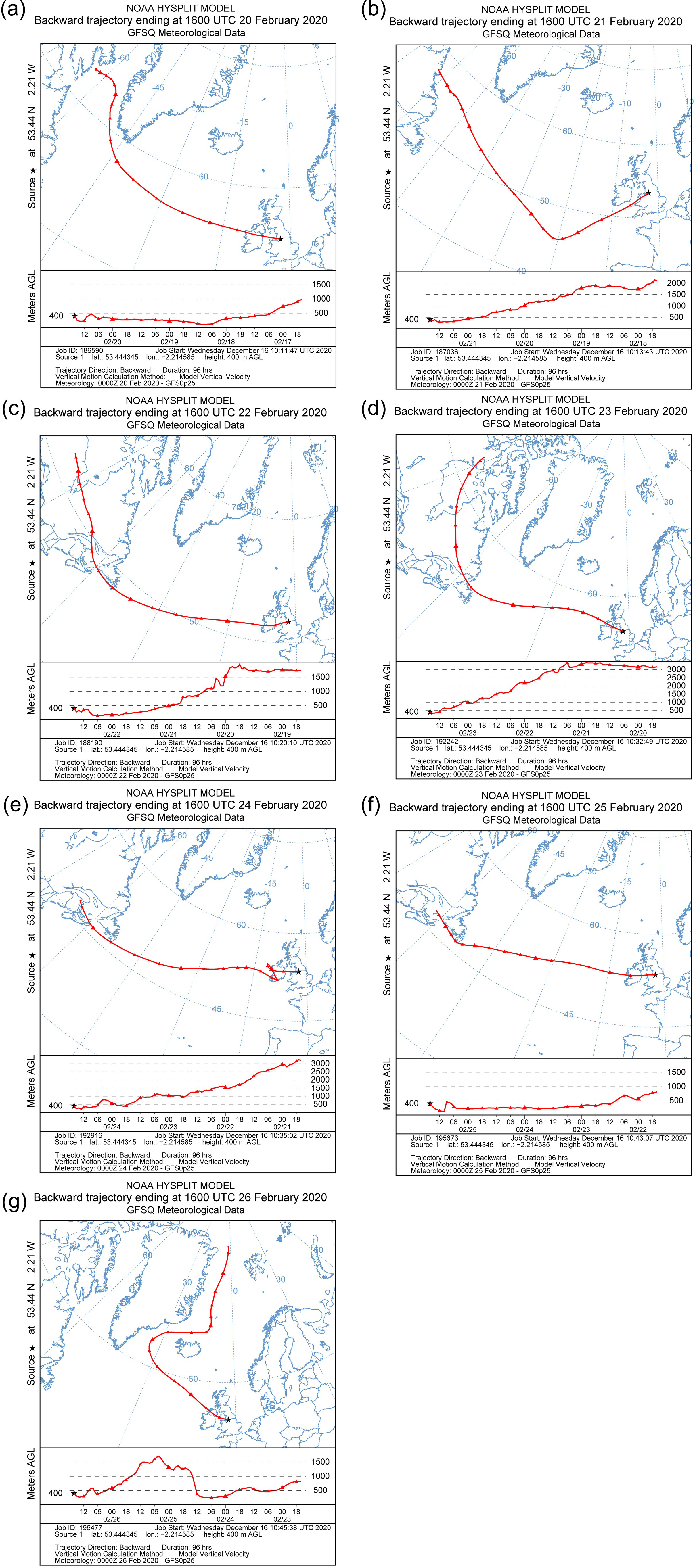
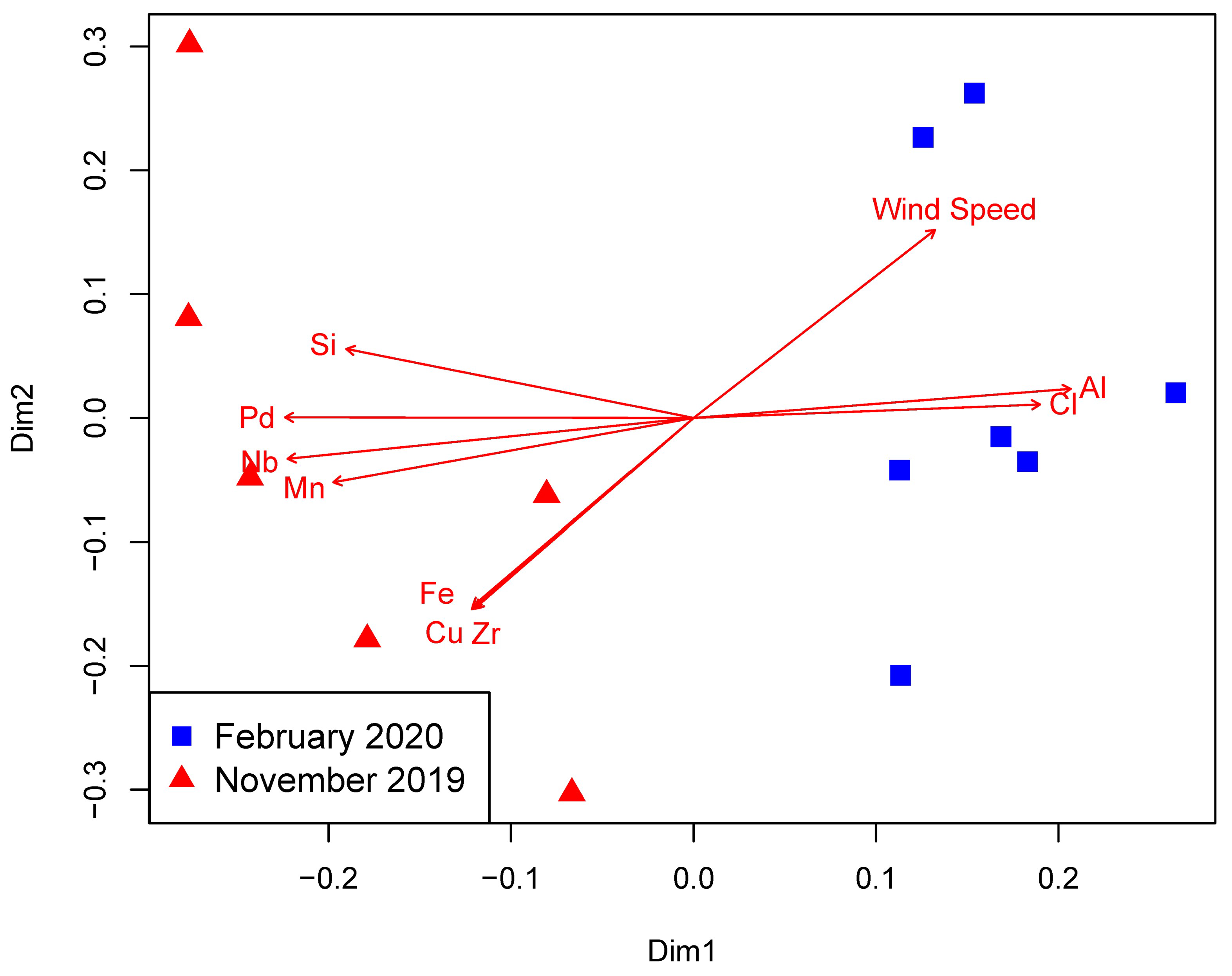
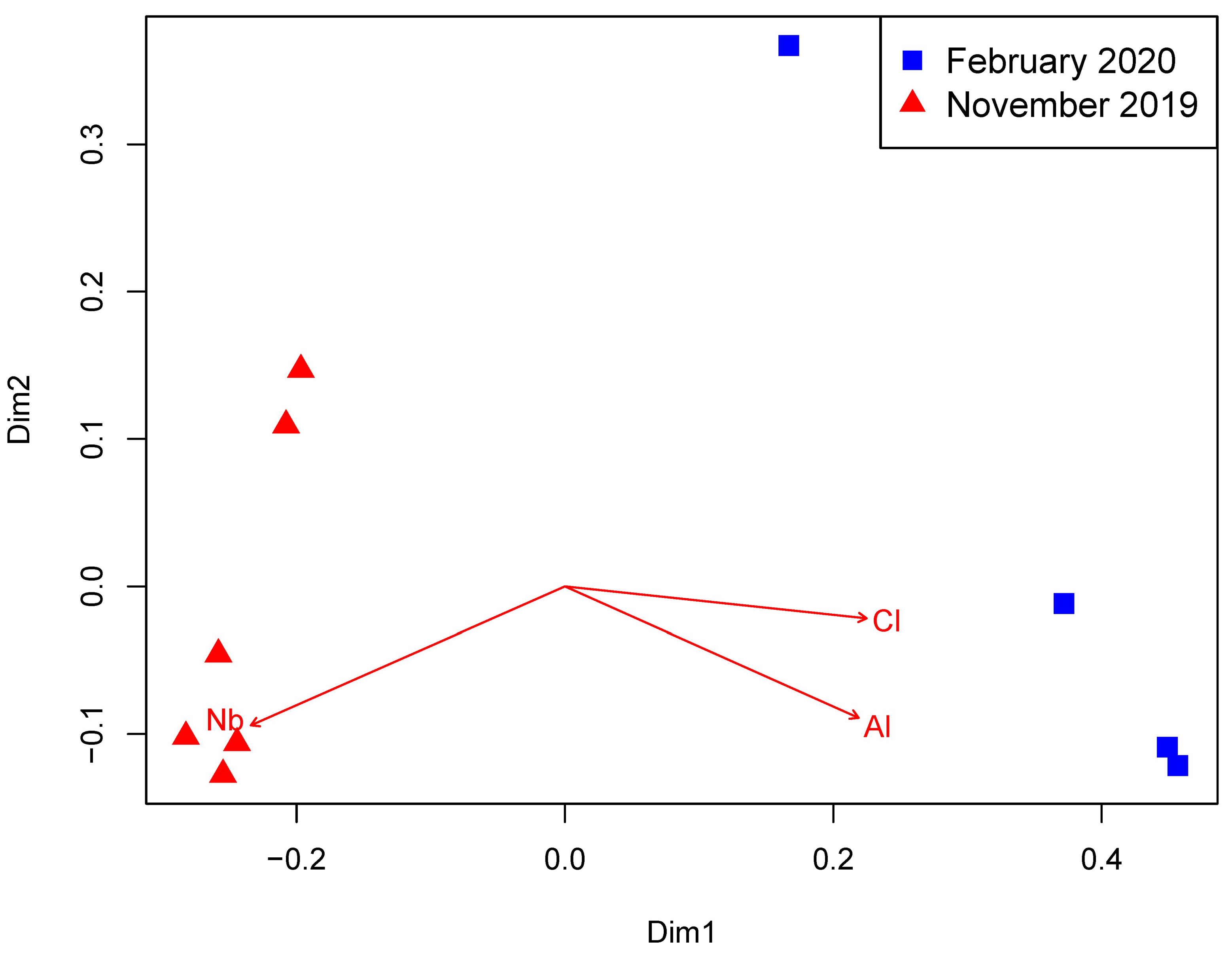
3.1. Environmental Parameters

Table S1 shows the average value of environmental parameters during each of the sample collection. The average temperature ranged from 5.4–7.8 °C when collecting November 2019 samples and 3.6–9.3 °C when collecting February 2020 samples (Table S1). The average humidity was over 80% in both of the sampling periods. The total precipitation rate was higher when collecting February 2020 samples (Table S2, Figure 1). Concentrations of heavy metals, for example, Ti, Mn, Fe, Cu, Zn, As, Zr, Nb, Pd, Te, Pb, and Bi, were significantly higher in the samples collected in November 2019 compared with those from February 2020 (Figure 1). In contrast, Cl concentrations were higher in the February 2020 samples.
Figure 2 and Figure 3 shows a series of 96-h Lagrangian back trajectories for airmasses arriving over the sampling site at an altitude of 400 m, calculated using the HYSPLIT (The Hybrid Single Particle Lagrangian Integrated Trajectory) modeling system with full 3D advection [45]. HYSPLIT was driven using GFS (Global Forecast System) 0.25-degree gridded meteorological reanalysis data. A 400 m receptor altitude was chosen to represent a layer consistent with the well-mixed planetary boundary layer at the measurement site (and high enough to prevent model particles colliding with the ground). The trajectories illustrate North-West marine-derived winds when collecting February 2020 samples and mostly land/continental origin of winds during November 2019 sampling. Environmental scanning electronic microscopy showed attachment of a C-containing feature (10 µm length, possibly a fungal spore) with NaCl in one of the February 2020 samples (Figure S5). This corresponds to the back trajectory of the winds coming from the North-West marine environment (Figure 3).
During November 2019, the particulate mass was generally below DEFRA (Department for Environment, Food and Rural Affairs) air quality limit values (Figure S1), however, some significant exceedances were observed, e.g., 03/11 and 06/11, where PM2.5 and PM10 exceed the DEFRA limits of 20 µg m−3 and 40 µg m−3, respectively; PM2.5 excided these limits during filter collection on the 16th and 17th of November. Fewer exceedances were observed during February 2020 (Figure S2), and none occurred during the filter sampling period. Figures S3 and S4 show polar concentration plots as a function of wind speed and direction for the two sampling periods, where the greatest aerosol loadings are typically observed at low wind speeds, suggesting local sources are important at the site. Significant enhancements in PM10 as compared with PM1 and PM2.5 were observed at higher wind speeds, and this was particularly prevalent during the February sampling period; the November period demonstrated an enhancement in PM10 from the South West which was not present in the PM1 loading, suggesting that there may be a separate and distinct source of large aerosol from this wind sector.

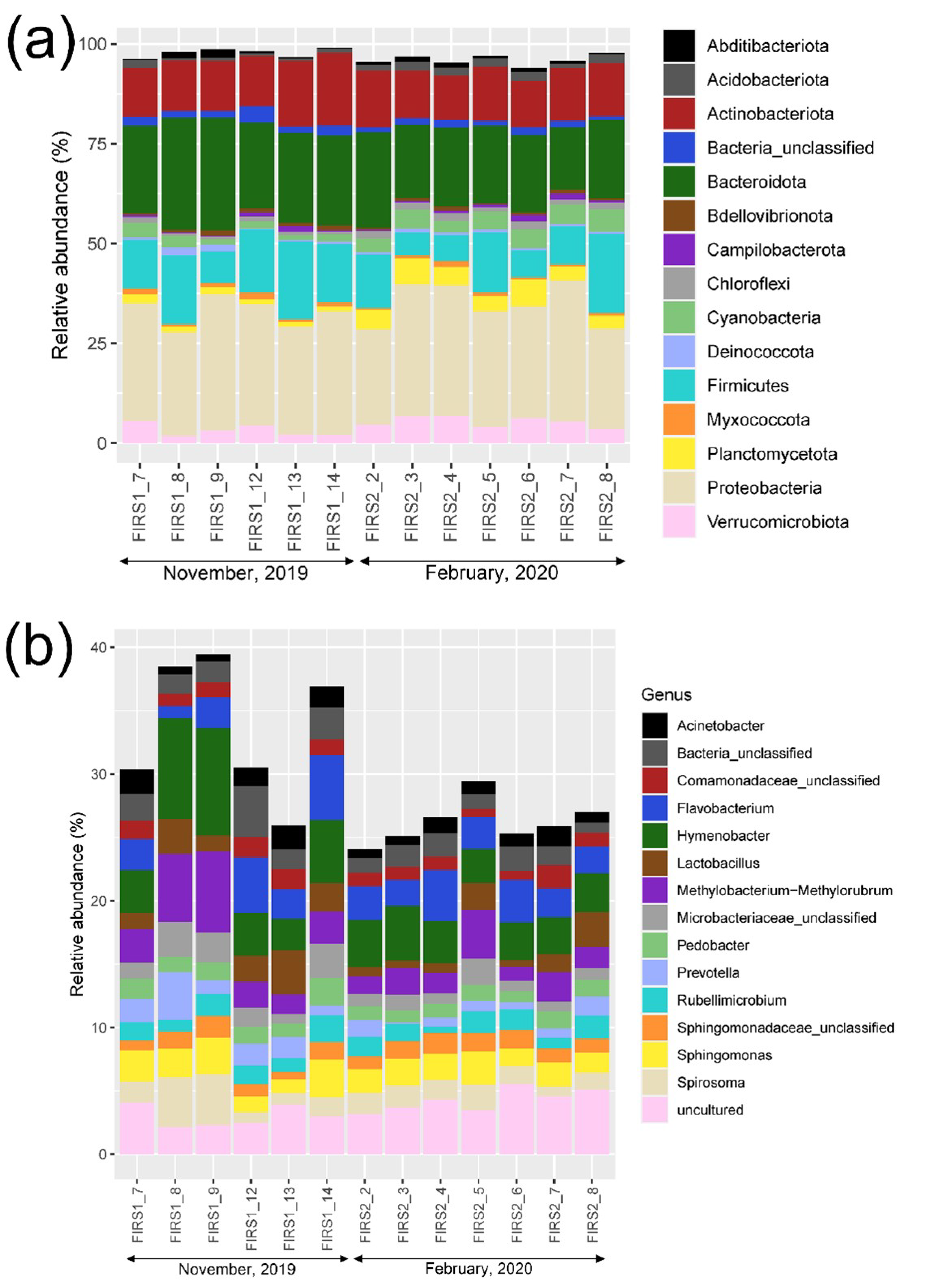
3.2. Prokaryotic Community Structure and Diversity

There was no significant difference in the absolute copy number of 16S rRNA genes between the November 2019 samples and February 2020 samples based on the qPCR results (Figure S6). The most abundant phylum on average was Proteobacteria, followed by Bacteroidota, Actinobacteria and Firmicutes (Figure 4a). The relative abundance of Bacteroidota was significantly higher in the November 2019 samples compared with the February 2020 samples, whereas the relative abundances of Verrucomicrobiota, Cyanobacteria, Planctomycetota, Acidobacteriota, and Chloroflexi were higher in the February 2020 samples (Table S3). The most abundant genus was Hymenobacter during both of the sampling periods. The second most abundant genus was Methylobacterium-Methylorubrum in November 2019 samples and Flavobacterium in February 2020 samples (Figure 4b).
Table 2 shows t-test (or Wilcoxon test) results of the 30 most abundant OTUs revealing significant differences in their relative abundance between the November 2019 samples and the February 2020 samples. The average relative abundance of OTU00020 was about six times higher in the November 2019 samples and had 100% similarity with Methylobacterium bullatum and Methylobacterium marchantiae based on blast search against the NCBI 16S rRNA sequence database. OTUs that had higher relative abundance in the February 2020 samples included marine environment associated taxa. For example, OTU000087, which was the most abundant archaeal OTU in the samples collected, was affiliated with “Marine Group II” based on the Silva database and had no blast matches with >80% similarity against the NCBI nt database. OTU000115, which was also relatively more abundant in the February 2020 samples, was affiliated with “SAR86_clade” based on the Silva database and had no blast match with > 90% similarity. OTU000147, which was affiliated with “Marinimicrobia ge” based on the Silva database and had no blast match with > 81% similarity, was also more abundant in the February 2020 samples.
Figure 5 shows a PCoA plot generated based on the Bray–Curtis distance of prokaryotic communities between the samples. There was a significant difference in prokaryotic community composition during the two different sampling periods based on the ANOSIM test (global R of 0.606 and p-value of 0.001). Environmental factors that were significantly correlated with the ordination are added as red arrows. Cl, Al, and wind speed were pointing towards the February 2020 samples, whereas Si, Pd, Nb, Mn, Fe, Cu, and Zr were pointing towards the November 2019 samples, confirming their significant association with the prokaryotic communities during each sampling period. In terms of alpha diversity, Shannon diversity values were significantly higher in the samples collected in February 2020 in comparison with November 2019 samples (Figure S7). However, there was no difference in the number of OTUs between the two sample sets.

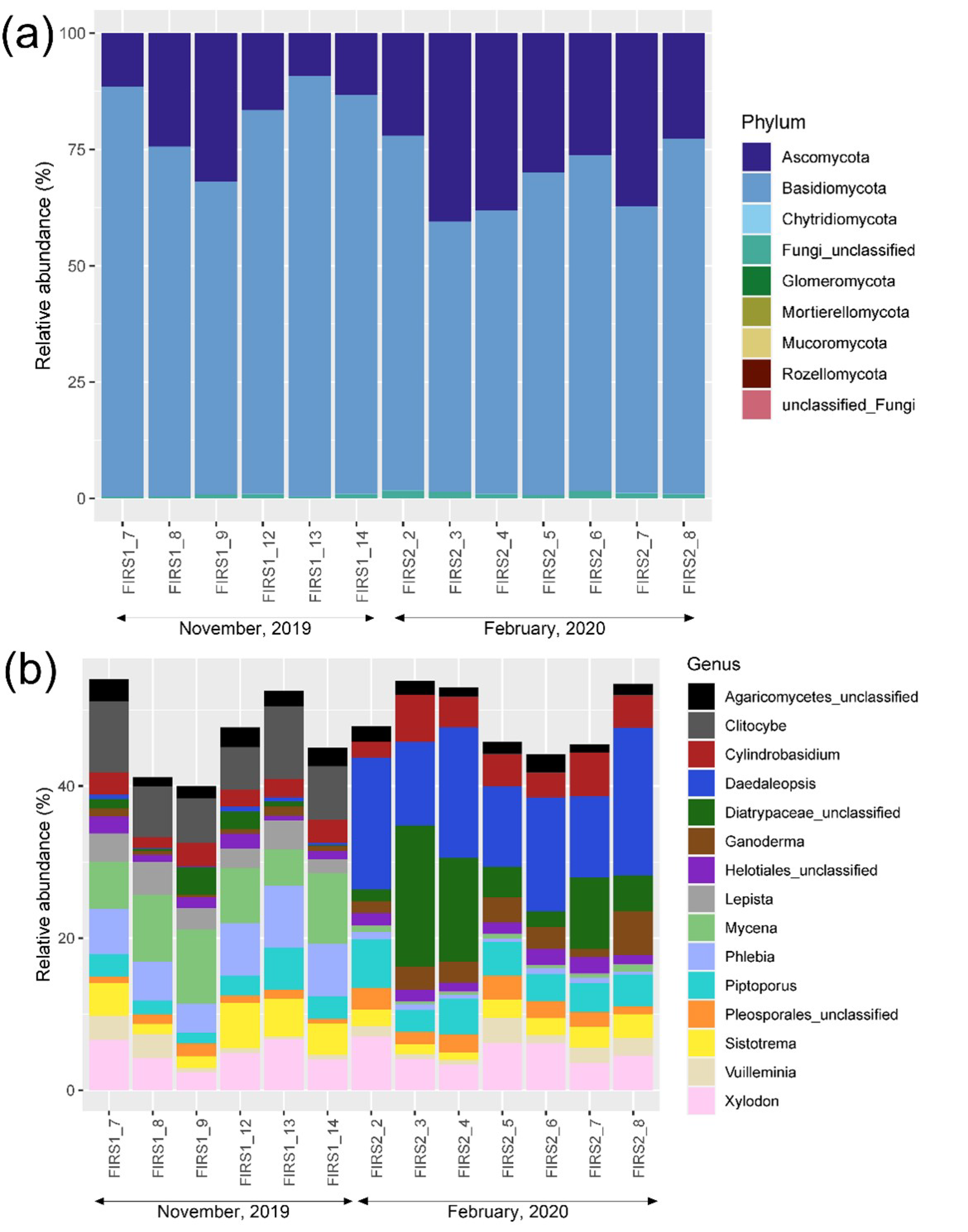
3.3. Fungal Community Structure and Diversity

The most abundant phylum on average was Basidiomycota followed by Ascomycota (Figure 6a). The relative abundance of Basidiomycota was significantly higher in the November 2019 samples compared with the February 2020 samples, whereas the relative abundance of Ascomycota was higher in the February 2020 samples (Table S4). The most abundant genus in the November 2019 samples was Mycena, followed by Clitocybe and Phlebia, whereas the most abundant genus in the February 2020 samples was Daedaleopsis, followed by Xylodon and Piptoporus (Figure 6b).
Table 3 shows the t-test (or Wilcoxon test) results of the 30 most abundant fungal OTUs that shows significant difference in their relative abundance between the November 2019 samples and the February 2020 samples. The relative abundance of fungal OTUs during the two different sampling time matched with their fruiting season (Supplementary Information). The OTUs annotated with fungal taxa that fruit all year round, for example, OTU000003 (Daedaleopsis confragosa) and Otu000009 (Cylindrobasdium evolvens), had generally higher relative abundance in the February 2020 samples, while the OTUs annotated with fungal taxa that fruit in autumn, for example, Otu000006 (Clitocybe nebularis), Otu000016 (Lepista_nuda) and Otu000026 (Paralepista flaccida), had generally higher relative abundance in the November 2019 samples.
Figure 7 shows a PCoA plot generated based on the Bray–Curtis distance of fungal communities between samples. There was a significant difference between the samples collected in November 2019 and the samples collected in February 2020 based on the ANOSIM test (global R of 1 and p-value of 0.002). Environmental factors that have significant correlation with the ordination are added as red arrows. Cl, Al, and wind speed arrows were pointing towards the February 2020 samples whereas Nb, Mn, Pd, Si, Fe, Cu, Zr, and CH4 were pointing towards the November 2019 samples. Shannon diversity and the number of fungal OTUs were significantly higher in the samples collected in November 2019 in comparison with February 2020 samples (Supplementary Figure S8).

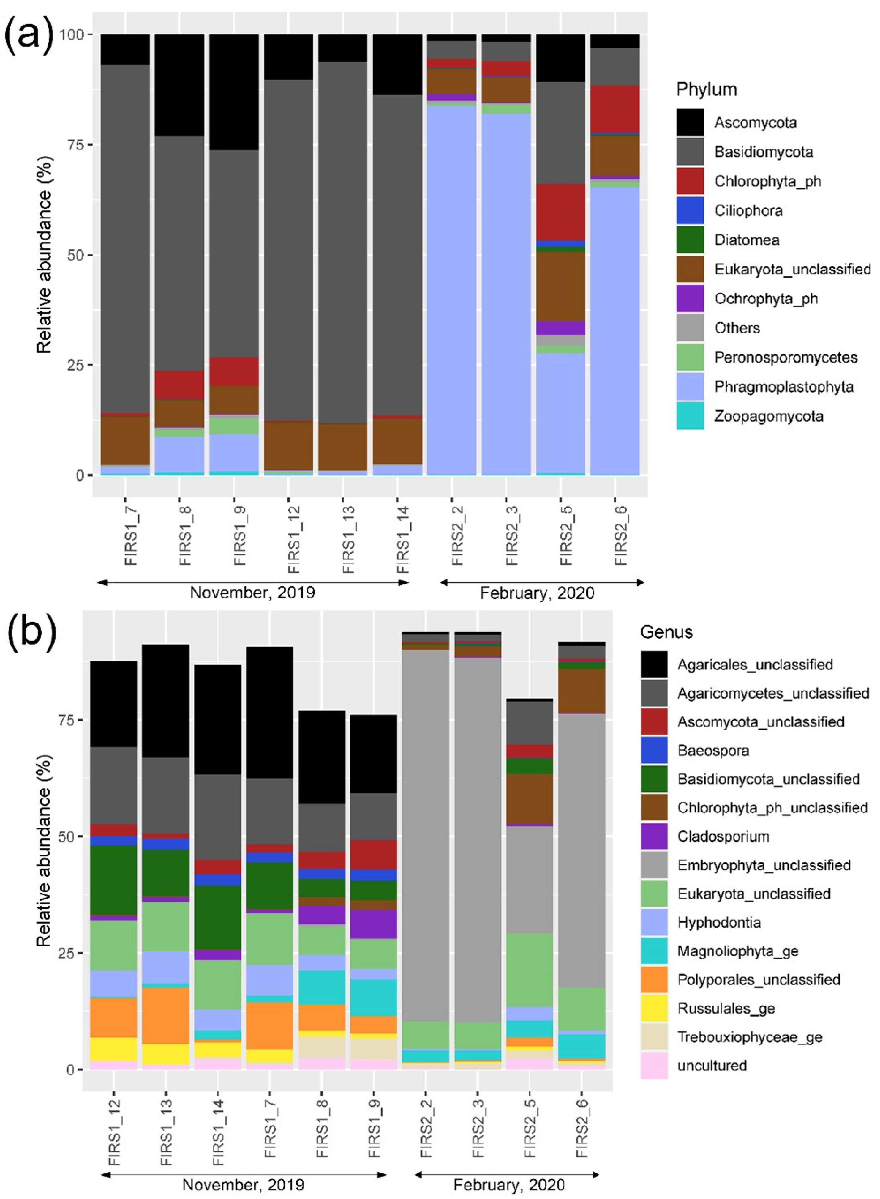
3.4. Eukaryotic Community Structure and Diversity

There was no significant difference in the absolute copy number of 16S rRNA genes between the November 2019 samples and February 2020 samples based on the qPCR results (Figure S9). Figure 8a shows the phylum level composition of eukaryotic communities classified based on the 18S rRNA gene in each of the sample. The most abundant phylum was Basidiomycota in the samples collected in November 2019. However, in contrast, the most abundant phylum in the samples collected in February 2020 was Phragmoplastophyta, which includes algae and land plants. The t-test (or Wilcoxon test) results showed that the relative abundance of Basidiomycota was significantly higher in the November 2019 samples compared with the February 2020 samples, whereas the relative abundances of Phragmoplastophyta and Diatomea were higher in the February 2020 samples (Table S5). Most of the sequences were unclassified at genus level (Figure 8b) based on the Silva database.
Table 4 shows the t-test (or Wilcoxon test) results of the 30 most abundant eukaryotic OTUs that show significant difference in their relative abundance between the November 2019 samples and the February 2020 samples. We found OTUs belonging to Taxus (Otu00011, Otu00136, Otu00258) of which pollens are common in the UK from mid-January until late April peaking in late February until mid-March (according to the pollen calendar produces by National Pollen and Aerobiology Research Unit, University of Worcester in 2012) to be relatively more abundant in the February 2020 samples. Otu00001, which had 100% similarity with species belonging to Lepista was relatively more abundant in the November 2019 samples than the February 2020 samples which corresponds with the ITS sequence data (Table 3). Otu00029 was classified as Chlorophyta and was relatively more abundant in the February 2020 samples compared with the November 2019 samples.
Figure 9 shows a PCoA plot generated based on the Bray–Curtis distance of eukaryotic communities between samples. There was a significant difference between the samples collected in November 2019 and the samples collected in February 2020 based on the ANOSIM test (global R of 0.996 and p-value of 0.005). Environmental factors that have significant correlation with the ordination are added as red arrows. Cl and Al arrows were pointing towards the February 2020 samples whereas Nb was pointing towards the November 2019 samples. There was no significant difference in Shannon diversity and in the number of fungal OTUs between the samples collected in November 2019 and in February 2020 (Figure S10).

4. Discussion

In this study, we used high throughput sequencing to monitor bioaerosols in Manchester, which is the second most populated city in the UK. The air quality based on PM2.5 and PM10 levels during sampling periods were in general under the limit. However, there were some days in November 2019 when PM2.5 level was over the air quality limit. The heavy metal concentrations were also higher in November 2019 sampling period. Regarding bioaerosol composition, the relative abundance of potential pathogens, for example, OTUs belonging to Methylobacterium, Streptococcus and Corynebacterium were higher in the November 2019 samples. Species belonging to Methylobacterium are known to be opportunistic pathogens which cause bacteremia in immunocompromised people [46,47]. Many species belonging to Streptococcus are pathogenic to humans, causing bacteremia, sepsis, pneumonia, and other diseases [48]. Corynebacterium include pathogenic bacterial species which cause a wide range of serious infections including diphtheria [49]. Considering these facts, the air quality in November 2019 seemed to be generally worse than February 2020, both in terms of non-bioaerosol and bioaerosol compositions.
The 5-year average data (Weather Spark, https://weatherspark.com/, accessed on 2 July 2022) show similar weather conditions in November and February in Manchester. During our sampling periods, the temperatures in November and February were similar, but wind directions, wind speeds and precipitation rates were different. In November 2019, the winds mostly originated from land/continent and the wind speed was slower than February 2020. In addition, the precipitation rate was lower than February 2020 sampling period. Considering these weather conditions, the air particles originating from anthropogenic activities (with high metal concentrations) seemed to persist for a long time during this sampling period. The higher relative abundance of the OTU belonging to Methylobacterium in November 2019 samples could also be linked with higher heavy metal concentrations as many of the species belonging to Methylobacterium are known to be heavy metal resistant [50,51].
During February 2020 sampling, Cl concentration was high which could be associated with the marine sourced winds. Agreeing with this, the relative abundance of marine environment-related taxa was higher in the February 2020 samples. For example, the relative abundance of Cyanobacteria and OTUs belonging to Marine Group II and SAR86 were higher in February 2020 samples. Species belonging to Cyanobacteria are mostly photosynthetic and are naturally found in various types of water environments. Marine Group II is a group of planktonic archaea predominantly found in ocean surface waters for which little genomic information is available and lacking cultured representatives [52]. SAR86 is one of the most abundant uncultured assemblages of bacteria found in ocean surface water [53].
In our study, fungal (spores) and plant (pollen) compositions were well explained by seasonal difference. Basidiomycetes of which the relative abundance was higher in the November 2019 samples are associated with decaying deciduous and coniferous trees and liter. There was a prominent difference in the eukaryotic phylum composition during the two sampling periods where in November 2019, most (> 50% on average) of the sequences were annotated as Basidiomycota whereas in February 2020, most (> 50% on average) of the sequences were annotated as Phragmoplastophyta. This corresponds with the results from Sharma Ghimire et al.’s study [54] which showed fungal loadings being highest in autumn and lowest in winter in an urban city in China.
There were some overlaps in the abundant phylum and genera found in our study with other urban and suburban areas. We found Proteobacteria, Bacteroidota, Actinobacteria and Firmicutes being the most dominant phyla. In Núñez et al.’s [55] study, Actinobacteria and Proteobacteria were dominant in the air of Madrid, Spain. Stewart et al. [23] studied airborne bacterial communities in Philadelphia, USA and found Proteobacteria to be the most dominant phylum. They also found Proteobacteria, Firmicutes, Actinobacteria and Bacteroidetes to be relatively more abundant in the urban area whereas Cyanobacteria, Tenericutes, Fusobacteria, and Deionococcus were more abundant in suburban area. Hymenobacteria, which was the most abundant genera in our samples, was also one of the dominant genera in a rapidly developing city in China [56]. A high abundance of Methylobacterium was observed in an suburban site in Toyama City, Japan [57].
The fungal compositions we found in this study were also to some extent similar to other urban studies. For example, in Sharma Ghimire et al.’s study [54], Clitocybe was one of the dominant fungal genera where it was abundant in spring and autumn and almost absent in summer and winter. In our study, the OTU annotated as Clitocybe nebularis was more abundant in November 2019 samples than in February 2020 samples, which agrees with their study. Woo et al. [58] studied wet and dry deposition of fungi in Seoul, South Korea and found Daedaleopsis being more abundant in wet deposition. In our study, Daedaleopsis was more abundant in February 2020 samples when the precipitation rate was higher.
There was a large proportion of Embryophyta in the February samples, but most of them were unclassified at the lower taxonomic levels when classified based on the Silva database. The reason is that Silva database itself does not include reference genomes of Embryophyta down to lower taxonomic levels. There is a need for a well-curated database for 18S rRNAs with high resolutions and until then, NCBI nt database could work as a substitute.

5. Conclusions

In this study, we used high throughput sequencing to monitor airborne prokaryotic, fungal, and eukaryotic communities in Manchester, UK. In November 2019 when the winds were slowly blowing from continent/land with less precipitation, the air quality was generally worse both in terms of biological and non-biological aerosol compositions than in February 2020. We found significant changes in the urban bioaerosol composition due to seasonal variation combined with local and long-range sources. In November 2019 there was higher relative abundance of an OTU that belongs to Methylobacterium which corresponds with higher heavy metal concentrations. In contrast, in February 2020 when the winds were blowing from the North-West marine environment, bacterial, archaeal and algae taxa were found to be abundant in marine/water environment, for example, Cyanobacteria, Marine Group II, SAR86_clade and Chlorophyta were relatively more abundant. In terms of fungal and other eukaryotic communities, bioaerosol compositions corresponded with seasonal differences. We found Basidiomycetes, which includes many species of decaying deciduous and coniferous trees and litter, relatively more abundant in November 2019 samples whereas more of plant-originated sequences (mostly undefined based on Silva database) were found in February 2020 samples. As for 18S rRNA sequencing, there is a demand for a well-curated database with high resolution. Overall, the results from this study suggest a potential application of bioaerosol profiling for tracing the source of atmospheric particles and influencing factors in an urban environment.

Supplementary Materials

The following supporting information can be downloaded at: https://www.mdpi.com/article/10.3390/atmos13081212/s1, Figure S1: PM1, PM2.5 and PM10 aerosol mass during the November 2019 sampling period; Figure S2: PM1, PM2.5 and PM10 aerosol mass during the February 2020 sampling period; Figure S3: Polar plot of PM1, PM2.5 and PM10 aerosol mass loadings for the November 2019 sampling period. Polar plots are a function of wind speed and wind direction, with concentric rings representing 1 m s−1 increments; Figure S4: Polar plot of PM1, PM2.5 and PM10 aerosol mass loadings for the February 2020 sampling period. Polar plots are a function of wind speed and wind direction, with concentric rings representing 1 m s−1 increments; Figure S5: Environmental scanning electronic microscopy image showing attachment of NaCl to a C containing feature; Figure S6: 16S/18S rRNA gene copy number per m3 of air in each sample; Figure S7: Shannon diversity and the number of prokaryotic OTUs found in the samples collected in November 2019 and in February 2020; Figure S8: Shannon diversity and the number of fungal OTUs found in the samples collected in November 2019 and in February 2020; Figure S9: 16S/18S rRNA gene copy number per m3 of air in each sample; Figure S10: Shannon diversity and the number of eukaryotic OTUs found in the samples collected in November 2019 and in February 2020; Table S1: Average value of each of the environmental parameter during sample collection; Table S2: t-test (or Wilcoxon rank sum test) results of environmental parameters compared between the two sampling periods; Table S3: t-test (or Wilcoxon rank sum test) result comparing the relative abundance of prokaryotic phylum between November 2019 samples and February 2020 samples; Table S4: t-test (or Wilcoxon rank sum test) result comparing the relative abundance of fungal phylum between November 2019 samples and February 2020 samples; Table S5: t-test (or Wilcoxon rank sum test) results comparing the relative abundance of eukaryotic phylum between November 2019 samples and February 2020 samples.

Author Contributions

Conceptualization, J.R.L., C.H.R., M.G. and G.A.; Methodology, N.M., M.G., I.C., C.B., H.C. and M.F.; Formal Analysis, H.S.; Investigation, N.M., I.C., C.B., H.S., M.G. and M.F.; Writing—Original Draft Preparation, H.S.; Writing—Review and Editing, C.H.R., I.C., J.R.L., M.G. and G.A.; Visualization, H.S.; Supervision, C.H.R., J.R.L. and M.G.; Project Administration, M.G.; Funding Acquisition, M.G. All authors have read and agreed to the published version of the manuscript.

Funding

The authors acknowledge the support of Natural Environment Research Council (NERC) via grant “Towards a UK Airborne Bioaerosol Climatology” (NE/S002049/1).

Data Availability Statement

The raw fastq formatted sequence files were archived in the NCBI SRA (sequence read archive) under project number of PRJNA731031.

Acknowledgments

Hokyung Song and Ian Crawford were funded by the NERC grant BIOARC, NE/S002049/1. The authors gratefully acknowledge the NOAA Air Resources Laboratory (ARL) for the provision of the HYSPLIT transport and dispersion model and READY website (https://www.ready.noaa.gov, assessed on 9 November 2020) used in this publication.

Conflicts of Interest

The authors declare no conflict of interest.

References

  1. Fröhlich-Nowoisky, J.; Kampf, C.J.; Weber, B.; Huffman, J.A.; Pöhlker, C.; Andreae, M.O.; Lang-Yona, N.; Burrows, S.M.; Gunthe, S.S.; Elbert, W.; et al. Bioaerosols in the Earth system: Climate, health, and ecosystem interactions. Atmos. Res. 2016, 182, 346–376. [Google Scholar] [CrossRef] [Green Version]
  2. Wittmaack, K.; Wehnes, H.; Heinzmann, U.; Agerer, R. An overview on bioaerosols viewed by scanning electron microscopy. Sci. Total Environ. 2005, 346, 244–255. [Google Scholar] [CrossRef] [PubMed]
  3. Crouzy, B.; Stella, M.; Konzelmann, T.; Calpini, B.; Clot, B. All-Optical automatic pollen identification: Towards an operational system. Atmos. Environ. 2016, 140, 202–212. [Google Scholar] [CrossRef]
  4. Šaulienė, I.; Šukienė, L.; Daunys, G.; Valiulis, G.; Vaitkevičius, L.; Matavulj, P.; Brdar, S.; Panic, M.; Sikoparija, B.; Clot, B.; et al. Automatic pollen recognition with the Rapid-E particle counter: The first-level procedure, experience and next steps. Atmos. Meas. Tech. 2019, 12, 3435–3452. [Google Scholar] [CrossRef] [Green Version]
  5. Crawford, I.; Topping, D.; Gallagher, M.; Forde, E.; Lloyd, J.R.; Foot, V.; Stopford, C.; Kaye, P. Detection of Airborne Biological Particles in Indoor Air Using a Real-Time Advanced Morphological Parameter UV-LIF Spectrometer and Gradient Boosting Ensemble Decision Tree Classifiers. Atmosphere 2020, 11, 1039. [Google Scholar] [CrossRef]
  6. Huffman, J.A.; Perring, A.E.; Savage, N.J.; Clot, B.; Crouzy, B.; Tummon, F.; Shoshanim, O.; Damit, B.; Schneider, J.; Sivaprakasam, V.; et al. Real-Time sensing of bioaerosols: Review and current perspectives. Aerosol Sci. Technol. 2020, 54, 465–495. [Google Scholar] [CrossRef] [Green Version]
  7. Amoo, A.E.; Babalola, O.O.; Stewart, F.J. Microbial Diversity of Temperate Pine and Native Forest Soils Profiled by 16S rRNA Gene Amplicon Sequencing. Microbiol. Resour. Announc. 2021, 10, e00298-21. [Google Scholar] [CrossRef]
  8. Jiang, H.; Chen, Y.; Hu, Y.; Wang, Z.; Lu, X. Soil Bacterial Communities and Diversity in Alpine Grasslands on the Tibetan Plateau Based on 16S rRNA Gene Sequencing. Front. Ecol. Evol. 2021, 9, 630722. [Google Scholar] [CrossRef]
  9. Semenov, M.V. Metabarcoding and Metagenomics in Soil Ecology Research: Achievements, Challenges, and Prospects. Biol. Bull. Rev. 2021, 11, 40–53. [Google Scholar] [CrossRef]
  10. Pearman, J.K.; Thomson-Laing, G.; Howarth, J.D.; Vandergoes, M.J.; Thompson, L.; Rees, A.; Wood, S.A. Investigating variability in microbial community composition in replicate environmental DNA samples down lake sediment cores. PLoS ONE 2021, 16, e0250783. [Google Scholar] [CrossRef]
  11. Ghate, S.D.; Shastry, R.P.; Arun, A.B.; Rekha, P.D. Unraveling the bacterial community composition across aquatic sediments in the Southwestern coast of India by employing high-throughput 16S rRNA gene sequencing. Reg. Stud. Mar. Sci. 2021, 46, 101890. [Google Scholar] [CrossRef]
  12. Zhu, C.; Zhang, J.; Nawaz, M.Z.; Mahboob, S.; Al-Ghanim, K.A.; Khan, I.A.; Lu, Z.; Chen, T. Seasonal succession and spatial distribution of bacterial community structure in a eutrophic freshwater Lake, Lake Taihu. Sci. Total Environ. 2019, 669, 29–40. [Google Scholar] [CrossRef]
  13. Cavaco, M.A.; St. Louis, V.L.; Engel, K.; St. Pierre, K.A.; Schiff, S.L.; Stibal, M.; Neufeld, J.D. Freshwater microbial community diversity in a rapidly changing High Arctic watershed. FEMS Microbiol. Ecol. 2019, 95, fiz161. [Google Scholar] [CrossRef]
  14. Malki, K.; Rosario, K.; Sawaya, N.A.; Székely, A.J.; Tisza, M.J.; Breitbart, M.; Moran, M.A. Prokaryotic and Viral Community Composition of Freshwater Springs in Florida, USA. mBio 2020, 11, e00436-20. [Google Scholar] [CrossRef] [Green Version]
  15. Ul-Hasan, S.; Bowers, R.M.; Figueroa-Montiel, A.; Licea-Navarro, A.F.; Beman, J.M.; Woyke, T.; Nobile, C.J. Community ecology across bacteria, archaea and microbial eukaryotes in the sediment and seawater of coastal Puerto Nuevo, Baja California. PLoS ONE 2019, 14, e0212355. [Google Scholar] [CrossRef] [Green Version]
  16. Wang, Y.; Liu, Y.; Wang, J.; Luo, T.; Zhang, R.; Sun, J.; Zheng, Q.; Jiao, N. Seasonal dynamics of bacterial communities in the surface seawater around subtropical Xiamen Island, China, as determined by 16S rRNA gene profiling. Mar. Pollut. Bull. 2019, 142, 135–144. [Google Scholar] [CrossRef]
  17. Schoch, C.L.; Seifert, K.A.; Huhndorf, S.; Robert, V.; Spouge, J.L.; Levesque, C.A.; Chen, W.; Bolchacova, E.; Voigt, K.; Crous, P.W.; et al. Nuclear ribosomal internal transcribed spacer (ITS) region as a universal DNA barcode marker for fungi. Proc. Natl. Acad. Sci. USA 2012, 109, 6241–6246. [Google Scholar] [CrossRef] [Green Version]
  18. Yuan, T.; Zhang, H.; Feng, Q.; Wu, X.; Zhang, Y.; McCarthy, A.J.; Sekar, R. Changes in Fungal Community Structure in Freshwater Canals across a Gradient of Urbanization. Water 2020, 12, 1917. [Google Scholar] [CrossRef]
  19. Sommermann, L.; Geistlinger, J.; Wibberg, D.; Deubel, A.; Zwanzig, J.; Babin, D.; Schlüter, A.; Schellenberg, I. Fungal community profiles in agricultural soils of a long-term field trial under different tillage, fertilization and crop rotation conditions analyzed by high-throughput ITS-Amplicon sequencing. PLoS ONE 2018, 13, e0195345. [Google Scholar] [CrossRef]
  20. Banerji, A.; Bagley, M.; Elk, M.; Pilgrim, E.; Martinson, J.; Santo Domingo, J. Spatial and temporal dynamics of a freshwater eukaryotic plankton community revealed via 18S rRNA gene metabarcoding. Hydrobiologia 2018, 818, 71–86. [Google Scholar] [CrossRef]
  21. Müller, C.A.; de Mattos Pereira, L.; Lopes, C.; Cares, J.; dos Anjos Borges, L.G.; Giongo, A.; Graeff-Teixeira, C.; Loureiro Morassutti, A. Meiofaunal diversity in the Atlantic Forest soil: A quest for nematodes in a native reserve using eukaryotic metabarcoding analysis. For. Ecol. Manag. 2019, 453, 117591. [Google Scholar] [CrossRef]
  22. Tanaka, D.; Sato, K.; Goto, M.; Fujiyoshi, S.; Maruyama, F.; Takato, S.; Shimada, T.; Sakatoku, A.; Aoki, K.; Nakamura, S. Airborne Microbial Communities at High-Altitude and Suburban Sites in Toyama, Japan Suggest a New Perspective for Bioprospecting. Front. Bioeng. Biotechnol. 2019, 7, 12. [Google Scholar] [CrossRef]
  23. Stewart, J.D.; Shakya, K.M.; Bilinski, T.; Wilson, J.W.; Ravi, S.; Choi, C.S. Variation of near surface atmosphere microbial communities at an urban and a suburban site in Philadelphia, PA, USA. Sci. Total Environ. 2020, 724, 138353. [Google Scholar] [CrossRef]
  24. Smith, D.J.; Ravichandar, J.D.; Jain, S.; Griffin, D.W.; Yu, H.; Tan, Q.; Thissen, J.; Lusby, T.; Nicoll, P.; Shedler, S.; et al. Airborne Bacteria in Earth’s Lower Stratosphere Resemble Taxa Detected in the Troposphere: Results From a New NASA Aircraft Bioaerosol Collector (ABC). Front. Microbiol. 2018, 9, 1752. [Google Scholar] [CrossRef]
  25. Kraaijeveld, K.; de Weger, L.A.; Ventayol García, M.; Buermans, H.; Frank, J.; Hiemstra, P.S.; den Dunnen, J.T. Efficient and sensitive identification and quantification of airborne pollen using next-generation DNA sequencing. Mol. Ecol. Resour. 2015, 15, 8–16. [Google Scholar] [CrossRef]
  26. Banchi, E.; Ametrano, C.G.; Stanković, D.; Verardo, P.; Moretti, O.; Gabrielli, F.; Lazzarin, S.; Borney, M.F.; Tassan, F.; Tretiach, M.; et al. DNA metabarcoding uncovers fungal diversity of mixed airborne samples in Italy. PLoS ONE 2018, 13, e0194489. [Google Scholar] [CrossRef]
  27. Xie, W.; Li, Y.; Bai, W.; Hou, J.; Ma, T.; Zeng, X.; Zhang, L.; An, T. The source and transport of bioaerosols in the air: A review. Front. Environ. Sci. Eng. 2020, 15, 44. [Google Scholar] [CrossRef]
  28. Smith, D.J.; Timonen, H.J.; Jaffe, D.A.; Griffin, D.W.; Birmele, M.N.; Perry, K.D.; Ward, P.D.; Roberts, M.S. Intercontinental Dispersal of Bacteria and Archaea by Transpacific Winds. Appl. Environ. Microbiol. 2013, 79, 1134–1139. [Google Scholar] [CrossRef] [Green Version]
  29. Mu, F.; Li, Y.; Lu, R.; Qi, Y.; Xie, W.; Bai, W. Source identification of airborne bacteria in the mountainous area and the urban areas. Atmos. Res. 2020, 231, 104676. [Google Scholar] [CrossRef]
  30. Knights, D.; Kuczynski, J.; Charlson, E.S.; Zaneveld, J.; Mozer, M.C.; Collman, R.G.; Bushman, F.D.; Knight, R.; Kelley, S.T. Bayesian community-wide culture-independent microbial source tracking. Nat. Methods 2011, 8, 761–763. [Google Scholar] [CrossRef] [Green Version]
  31. Taleghani, M. Air Pollution within Different Urban Forms in Manchester, UK. Climate 2022, 10, 26. [Google Scholar] [CrossRef]
  32. Gollakota, A.R.K.; Gautam, S.; Santosh, M.; Sudan, H.A.; Gandhi, R.; Sam Jebadurai, V.; Shu, C.-M. Bioaerosols: Characterization, pathways, sampling strategies, and challenges to geo-environment and health. Gondwana Res. 2021, 99, 178–203. [Google Scholar] [CrossRef]
  33. Ravindra, K.; Wauters, E.; Van Grieken, R. Variation in particulate PAHs levels and their relation with the transboundary movement of the air masses. Sci. Total Environ. 2008, 396, 100–110. [Google Scholar] [CrossRef] [Green Version]
  34. Huang, S.; Wu, Z.; Poulain, L.; van Pinxteren, M.; Merkel, M.; Assmann, D.; Herrmann, H.; Wiedensohler, A. Source apportionment of the organic aerosol over the Atlantic Ocean from 53° N to 53° S: Significant contributions from marine emissions and long-range transport. Atmos. Chem. Phys. 2018, 18, 18043–18062. [Google Scholar] [CrossRef] [Green Version]
  35. Barker, P.A.; Allen, G.; Flynn, M.; Riddick, S.; Pitt, J.R. Measurement of Recreational N2o Emissions from an Urban Environment in Manchester, UK. 2022. Available online: https://ssrn.com/abstract=4071514 (accessed on 2 July 2022).
  36. Masella, A.P.; Bartram, A.K.; Truszkowski, J.M.; Brown, D.G.; Neufeld, J.D. PANDAseq: Paired-End assembler for illumina sequences. BMC Bioinform. 2012, 13, 31. [Google Scholar] [CrossRef] [Green Version]
  37. Schloss, P.D.; Westcott, S.L.; Ryabin, T.; Hall, J.R.; Hartmann, M.; Hollister, E.B.; Lesniewski, R.A.; Oakley, B.B.; Parks, D.H.; Robinson, C.J.; et al. Introducing mothur: Open-Source, Platform-Independent, Community-Supported Software for Describing and Comparing Microbial Communities. Appl. Environ. Microbiol. 2009, 75, 7537–7541. [Google Scholar] [CrossRef] [Green Version]
  38. Rognes, T.; Flouri, T.; Nichols, B.; Quince, C.; Mahé, F. VSEARCH: A versatile open source tool for metagenomics. PeerJ 2016, 4, e2584. [Google Scholar] [CrossRef]
  39. Quast, C.; Pruesse, E.; Yilmaz, P.; Gerken, J.; Schweer, T.; Yarza, P.; Peplies, J.; Glöckner, F.O. The SILVA ribosomal RNA gene database project: Improved data processing and web-based tools. Nucleic Acids Res. 2012, 41, D590–D596. [Google Scholar] [CrossRef]
  40. Westcott, S.L.; Schloss, P.D.; McMahon, K.; Watson, M.; Pollard, K. OptiClust, an Improved Method for Assigning Amplicon-Based Sequence Data to Operational Taxonomic Units. Msphere 2017, 2, e00073-17. [Google Scholar] [CrossRef] [Green Version]
  41. Altschul, S.F.; Gish, W.; Miller, W.; Myers, E.W.; Lipman, D.J. Basic local alignment search tool. J. Mol. Biol. 1990, 215, 403–410. [Google Scholar] [CrossRef]
  42. Sayers, E.W.; Agarwala, R.; Bolton, E.E.; Brister, J.R.; Canese, K.; Clark, K.; Connor, R.; Fiorini, N.; Funk, K.; Hefferon, T.; et al. Database resources of the National Center for Biotechnology Information. Nucleic Acids Res. 2018, 47, D23–D28. [Google Scholar] [CrossRef] [Green Version]
  43. Dixon, P. VEGAN, a package of R functions for community ecology. J. Veg. Sci. 2003, 14, 927–930. [Google Scholar] [CrossRef]
  44. Clarke, K.; Gorley, R. PRIMER: Getting started with v6.; PRIMER-E Ltd.: Plymouth, UK, 2005; Volume 931, p. 932. [Google Scholar]
  45. Stein, A.F.; Draxler, R.R.; Rolph, G.D.; Stunder, B.J.B.; Cohen, M.D.; Ngan, F. NOAA’s HYSPLIT Atmospheric Transport and Dispersion Modeling System. Bull. Am. Meteorol. Soc. 2015, 96, 2059–2077. [Google Scholar] [CrossRef]
  46. Lai, C.C.; Cheng, A.; Liu, W.L.; Tan, C.K.; Huang, Y.T.; Chung, K.P.; Lee, M.R.; Hsueh, P.R. Infections caused by unusual Methylobacterium species. J. Clin. Microbiol. 2011, 49, 3329–3331. [Google Scholar] [CrossRef] [Green Version]
  47. Szwetkowski, K.J.; Falkinham, J.O. Methylobacterium spp. as Emerging Opportunistic Premise Plumbing Pathogens. Pathogens 2020, 9, 149. [Google Scholar] [CrossRef] [Green Version]
  48. Krzyściak, W.; Pluskwa, K.K.; Jurczak, A.; Kościelniak, D. The pathogenicity of the Streptococcus genus. Eur. J. Clin. Microbiol. Infect. Dis. 2013, 32, 1361–1376. [Google Scholar] [CrossRef] [Green Version]
  49. Rogers, E.A.; Das, A.; Ton-That, H. Adhesion by pathogenic corynebacteria. Adv. Exp. Med. Biol. 2011, 715, 91–103. [Google Scholar] [CrossRef]
  50. Idris, R.; Kuffner, M.; Bodrossy, L.; Puschenreiter, M.; Monchy, S.; Wenzel, W.W.; Sessitsch, A. Characterization of Ni-tolerant methylobacteria associated with the hyperaccumulating plant Thlaspi goesingense and description of Methylobacterium goesingense sp. nov. Syst. Appl. Microbiol. 2006, 29, 634–644. [Google Scholar] [CrossRef]
  51. Photolo, M.M.; Sitole, L.; Mavumengwana, V.; Tlou, M.G. Genomic and Physiological Investigation of Heavy Metal Resistance from Plant Endophytic Methylobacterium radiotolerans MAMP 4754, Isolated from Combretum erythrophyllum. Int. J. Environ. Res. Public Health 2021, 18, 997. [Google Scholar] [CrossRef]
  52. Rinke, C.; Rubino, F.; Messer, L.F.; Youssef, N.; Parks, D.H.; Chuvochina, M.; Brown, M.; Jeffries, T.; Tyson, G.W.; Seymour, J.R.; et al. A phylogenomic and ecological analysis of the globally abundant Marine Group II archaea (Ca. Poseidoniales ord. nov.). ISME J. 2019, 13, 663–675. [Google Scholar] [CrossRef] [Green Version]
  53. Dupont, C.L.; Rusch, D.B.; Yooseph, S.; Lombardo, M.-J.; Richter, R.A.; Valas, R.; Novotny, M.; Yee-Greenbaum, J.; Selengut, J.D.; Haft, D.H.; et al. Genomic insights to SAR86, an abundant and uncultivated marine bacterial lineage. ISME J. 2012, 6, 1186–1199. [Google Scholar] [CrossRef] [PubMed] [Green Version]
  54. Sharma Ghimire, P.; Joshi, D.R.; Tripathee, L.; Chen, P.; Sajjad, W.; Kang, S. Seasonal taxonomic composition of microbial communal shaping the bioaerosols milieu of the urban city of Lanzhou. Arch. Microbiol. 2022, 204, 222. [Google Scholar] [CrossRef] [PubMed]
  55. Núñez, A.; Amo de Paz, G.; Rastrojo, A.; Ferencova, Z.; Gutiérrez-Bustillo, A.M.; Alcamí, A.; Moreno, D.A.; Guantes, R. Temporal patterns of variability for prokaryotic and eukaryotic diversity in the urban air of Madrid (Spain). Atmos. Environ. 2019, 217, 116972. [Google Scholar] [CrossRef]
  56. Li, H.; Zhou, X.-Y.; Yang, X.-R.; Zhu, Y.-G.; Hong, Y.-W.; Su, J.-Q. Spatial and seasonal variation of the airborne microbiome in a rapidly developing city of China. Sci. Total Environ. 2019, 665, 61–68. [Google Scholar] [CrossRef]
  57. Tanaka, D.; Fujiyoshi, S.; Maruyama, F.; Goto, M.; Koyama, S.; Kanatani, J.-i.; Isobe, J.; Watahiki, M.; Sakatoku, A.; Kagaya, S.; et al. Size resolved characteristics of urban and suburban bacterial bioaerosols in Japan as assessed by 16S rRNA amplicon sequencing. Sci. Rep. 2020, 10, 12406. [Google Scholar] [CrossRef]
  58. Woo, C.; An, C.; Xu, S.; Yi, S.-M.; Yamamoto, N. Taxonomic diversity of fungi deposited from the atmosphere. ISME J. 2018, 12, 2051–2060. [Google Scholar] [CrossRef] [Green Version]
Figure 1. Boxplots of environmental parameters that were significantly different between November 2019 samples and February 2020 samples.
Atmosphere 13 01212 g001
Figure 2. 96 h HYSPLIT Lagrangian back trajectories of air at the start point of each sample collected in November 2019. (a) “FIRS1_7”, (b) “FIRS1_8”, (c) “FIRS1_9”, (d) “FIRS1_12”, (e) “FIRS1_13” and (f) “FIRS1_14”.
Atmosphere 13 01212 g002
Figure 3. 96 h HYSPLIT Lagrangian back trajectories of air at the start point of each sample collected in February 2020. (a) “FIRS2_2”, (b) “FIRS2_3”, (c) “FIRS2_4”, (d) “FIRS2_5”, (e) “FIRS2_6”, (f) “FIRS2_7” and (g) “FIRS2_8”.
Atmosphere 13 01212 g003
Figure 4. The 15 most abundant prokaryotic phyla (a) and genera (b) in the samples.
Atmosphere 13 01212 g004
Figure 5. PCoA (principal coordinate analysis) plot of prokaryotic communities. Environmental factors that have significant correlation with the ordination (with p value lower than 0.01 and R-square value larger than 0.5) based on permutation tests are shown as red arrows.
Atmosphere 13 01212 g005
Figure 6. The 15 most abundant fungal phyla (a) and genera (b) in the samples.
Atmosphere 13 01212 g006
Figure 7. PCoA (principal coordinate analysis) plot of fungal communities. Environmental factors that have significant correlation with the ordination (with p value lower than 0.01 and R-square value larger than 0.5) based on permutation tests are shown as red arrows.
Atmosphere 13 01212 g007
Figure 8. The 15 most abundant eukaryotic phyla (a) and genera (b) in the samples.
Atmosphere 13 01212 g008
Figure 9. PCoA (principal coordinate analysis) plot of eukaryotic communities. Environmental factors that have significant correlation with the ordination (with p value lower than 0.01 and R-square value larger than 0.5) based on permutation tests are shown as red arrows.
Atmosphere 13 01212 g009
Table 1. Sample information.
Sample IDStart TimeEnd Time
FIRS1_712 November 2019 13:1613 November 2019 13:15
FIRS1_813 November 2019 13:1614 November 2019 13:15
FIRS1_914 November 2019 13:1615 November 2019 10:40
FIRS1_1215 November 2019 10:4016 November 2019 10:40
FIRS1_1316 November 2019 10:4017 November 2019 10:40
FIRS1_1417 November 2019 10:4018 November 2019 10:20
FIRS2_220 February 2020 16:2521 February 2020 16:25
FIRS2_321 February 2020 16:2522 February 2020 16:25
FIRS2_422 February 2020 16:2523 February 2020 16:25
FIRS2_523 February 2020 16:2524 February 2020 16:25
FIRS2_624 February 2020 16:2525 February 2020 16:25
FIRS2_725 February 2020 16:2526 February 2020 16:25
FIRS2_826 February 2020 16:2527 February 2020 16:25
Table 2. t-test (or Wilcoxon test) results of the 30 most abundant prokaryotic OTUs that show significant difference in their relative abundance between the November 2019 samples and the February 2020 samples. Their taxonomic annotation based on the Silva database and their BLAST result against NCBI nt database (best hit score, classified down to species level) are shown together.
OTU IDp ValueNov_2019
Average (%)
Feb_2020
Average (%)
Taxonomy Based on the Silva DatabaseBLAST against NCBI nt Database
TaxonomySimilarity (%)E-Value
Otu0000200.0451.1360.187Methylobacterium-MethylorubrumMethylobacterium bullatum, Methylobacterium marchantiae1006 × 10−120
Otu0000140.0170.7620.470RubellimicrobiumRubellimicrobium aerolatum1009 × 10−112
Otu0000190.0320.6480.433PedobacterPedobacter miscanthi, Pedobacter helvus, and etc. 1002 × 10−125
Otu0000480.0160.6540.046Bacteria_unclassifiedCalycina alstrupii88.299 × 10−73
Otu0000470.0120.4060.201StreptococcusStreptococcus gallolyticus, Streptococcus pasteurianus, and etc. 1008 × 10−125
Otu0000540.0180.6040.021Moraxellaceae_geAgitococcus lubricus97.623 × 10−117
Otu0000580.0200.3670.161LactobacillusLactobacillus johnsonii, Lactobacillus paragasseri, and etc. 1002 × 10−125
Otu0000530.0370.0970.345RickettsiellaDiplorickettsia massiliensis 20B 98.023 × 10−118
Otu0000990.0360.3310.076PrevotellaPrevotella hominis99.61 × 10−123
Otu0000890.0180.3710.039SpirosomaSpirosoma oryzae96.832 × 10−114
Otu0001020.0030.2830.103AureimonasAureimonas glaciei1002 × 10−125
Otu0001220.0360.2960.062PseudomonasPaucimonas lemoignei, Pseudomonas versuta, and etc. 1002 × 10−125
Otu0000900.0050.0510.270unculturedRoseimicrobium gellanilyticum87.36 × 10−82
Otu0001200.0230.3150.041Staphylococcaceae_unclassifiedMammaliicoccus fleurettii, Mammaliicoccus sciuri, and etc. 1002 × 10−125
Otu0001080.0300.2120.115DyadobacterDyadobacter frigoris, Dyadobacter hamtensis99.61 × 10−123
Otu0001290.0410.2380.090ChryseobacteriumChryseobacterium solani, Epilithonimonas ginsengisoli, and etc. 1002 × 10−125
Otu0001110.0380.2060.115CorynebacteriumCorynebacterium freneyi, Corynebacterium xerosis1007 × 10−126
Otu0000910.0370.0630.215PseudarcobacterArcobacter suis, Arcobacter caeni1002 × 10−125
Otu0000870.0020.0000.251Marine_Group_II_geMethanobrevibacter cuticularis79.453 × 10−54
Otu0001480.0130.1740.080SpirosomaSpirosoma pomorum96.832 × 10−114
Otu0001150.0110.0230.208SAR86_clade_gePseudomonas nabeulensis89.338 × 10−87
Otu0001430.0030.0140.194Corynebacteriales_unclassifiedRhodococcus aerolatus1002 × 10−125
Otu0002020.0100.2010.032Comamonadaceae_unclassifiedXylophilus rhododendri, Ramlibacter rhizophilus, and etc. 1002 × 10−125
Otu0001410.0010.0330.173SphingomonasSphingomonas flava99.61 × 10−123
Otu0001470.0330.0370.155Marinimicrobia__geAcinetobacter piscicola, Acinetobacter marinus80.572 × 10−57
Otu0001620.0430.0240.164Scytonema_UTEX_2349Hassallia antarctica99.61 × 10−123
Otu0002460.0250.1690.0351174-901-12Lichenihabitans psoromatis, Beijerinckia mobilis95.634 × 10−110
Otu0001830.0040.0030.164Crocinitomicaceae_unclassifiedWandonia haliotis95.634 × 10−110
Otu0002300.0160.0050.155Cyanobacteriia_unclassifiedLobosphaera incisa87.75 × 10−83
Otu0002060.0350.0230.136Calothrix_PCC-6303Macrochaete lichenoides99.211 × 10−122
Table 3. t-test (or Wilcoxon test) results of the 30 most abundant fungal OTUs that shows significant difference in their relative abundance between the November 2019 samples and the February 2020 samples. Their taxonomic annotation based on the UNITE database and their BLAST result against NCBI nt database (best hit score, classified down to species level) are shown together.
OTU IDp ValueNov_2019
Average (%)
Feb_2020
Average (%)
Taxonomy Based on the UNITE DatabaseBLAST against NCBI nt Database
TaxonomySimilarity (%)E-Value
Otu0000030.0000.40514.467Daedaleopsis_unclassifiedDaedaleopsis confragosa, Lenzites betulinus, and etc.1000
Otu0000040.0006.0170.522Phlebia_unclassifiedPhlebia radiata1000
Otu0000060.0026.2250.001Clitocybe_nebularisLeucopaxillus tricolor, Lepista nebularis1000
Otu0000090.0182.4684.198Cylindrobasidium_evolvensPolyporus gayanus99.5670
Otu0000100.0034.1920.006Mycena_metataMycena arcangeliana98.9660
Otu0000130.0292.6210.600Sistotrema_oblongisporumClavulina cristata83.2522.91 × 10−95
Otu0000160.0012.4510.036Lepista_nudaLepista nuda99.2080
Otu0000170.0060.6092.896Ganoderma_australeGanoderma australe99.7280
Otu0000220.0011.6350.000Infundibulicybe_geotropaAmpulloclitocybe clavipes94.018.94 × 10−160
Otu0000230.0171.5030.061Peniophora_unclassifiedPeniophora piceae96.9612.34 × 10−170
Otu0000260.0011.5100.000Paralepista_flaccidaParalepista gilva99.730
Otu0000290.0071.1640.325Radulomyces_molarisCuphophyllus colemannianus90.5171.63 × 10−77
Otu0000310.0350.4870.268Coprinellus_micaceusCoprinellus micaceus, Coprinus rufopruinatus1000
Otu0000340.0010.3641.184Heterobasidion_unclassifiedPodoscypha multizonata, Podoscypha involuta1000
Otu0000350.0010.7640.101Hypholoma_fasciculareHypholoma fasciculare1000
Otu0000370.0341.0300.088Trechispora_byssinellaTrechispora byssinella99.1890
Otu0000400.0330.4401.002Antrodia_xanthaAmyloporia xantha, Antrodia xantha1000
Otu0000420.0010.2001.328Polyporaceae_unclassifiedTrametes gibbosa1000
Otu0000430.0010.0581.506Diatrypaceae_unclassifiedEutypa lata1009.68 × 10−169
Otu0000440.0410.5140.776Russulales_unclassifiedPeniophora incarnata1000
Otu0000450.0000.9900.034Clitocybe_unclassifiedClitocybe vibecina99.7330
Otu0000460.0170.4540.856Xenasmatella_unclassifiedPhlebiella borealis98.8641.74 × 10−176
Otu0000480.0060.0691.288Xylariales_unclassifiedEutypa lata1002.70 × 10−169
Otu0000490.0120.4420.716Hyphodontia_pallidulaHyphodontia pallidula99.4460
Otu0000500.0010.1931.048Pleosporales_unclassifiedPhaeosphaeria caricicola94.3757.65 × 10−135
Otu0000510.0010.8860.000Rhodocollybia_butyraceaRhodocollybia butyracea99.5420
Otu0000520.0020.2700.885Resinicium_bicolorResinicium bicolor1000
Otu0000540.0030.2020.665Flammulina_velutipesFlammulina velutipes1000
Otu0000560.0010.5870.105Pleurotus_ostreatusPleurotus sapidus, Pleurotus ostreatus, and etc.1000
Otu0000580.0270.6060.042Hyaloscyphaceae_unclassifiedLachnum virgineum93.6313.52 × 10−128
Table 4. t-test (or Wilcoxon test) results of the 30 most abundant eukaryotic OTUs that shows significant difference in their relative abundance between the November 2019 samples and the February 2020 samples. Their taxonomic annotation based on the Silva database and their BLAST result against NCBI nt database (best hit score, classified down to species level) are shown together.
OTU IDp ValueNov_2019
Average (%)
Feb_2020
Average (%)
Taxonomy Based on the Silva DatabaseBLAST against NCBI nt Database
TaxonomySimilarity (%)E-Value
Otu000110.0060.00056.006Embryophyta_unclassifiedTaxus wallichiana1003.06 × 10−49
Otu000010.00017.6910.270Agaricales_unclassifiedLepista sordida, Lepista saeva, etc.1001.09 × 10−48
Otu000020.0146.5630.323Polyporales_unclassifiedFomitopsis pinicola, Antrodia albida, etc.1001.09 × 10−48
Otu000030.0135.6110.749Basidiomycota_unclassifiedSistotrema brinkmannii, Sistotrema oblongisporum1001.09 × 10−48
Otu000040.0084.1371.057HyphodontiaHyphodontia rimosissima95.4132.37 × 10−40
Otu000290.0380.7085.812Chlorophyta_ph_unclassifiedTrebouxia impressa1001.09 × 10−48
Otu000060.0023.2490.092Agaricomycetes_unclassifiedPhlebia radiata1001.09 × 10−48
Otu000080.0112.8790.377Russulales_gePeniophora nuda98.1651.82 × 10−46
Otu000120.0002.1930.038BaeosporaBaeospora myosura1001.09 × 10−48
Otu000150.0142.0130.275Agaricomycetes_unclassifiedRogersella griseliniae95.4132.37 × 10−40
Otu000160.0112.0770.000Magnoliophyta_geParietaria judaica1008.61 × 10−50
Otu000170.0231.7140.367Eukaryota_unclassifiedSterigmatomyces halophilu90.9915.16 × 10−32
Otu001360.0060.0002.890Eukaryota_unclassifiedTaxus wallichiana99.091.00 × 10−45
Otu000240.0131.2180.005Basidiomycota_unclassifiedChamaeota sinica93.5785.12 × 10−37
Otu000280.0380.9420.199Eukaryota_unclassifiedHyphodontia crustosa92.6612.38 × 10−35
Otu000350.0250.7440.248Agaricomycetes_unclassifiedBurgoa anomala, Sistotrema octosporum, etc.1001.09 × 10−48
Otu000310.0020.7260.162Agaricomycetes_unclassifiedRogersella griseliniae91.8181.11 × 10−33
Otu000320.0130.8020.005Agaricales_unclassifiedMycena galericulata98.1652.35 × 10−45
Otu002580.0060.0001.068Embryophyta_unclassifiedTaxus wallichiana99.091.00 × 10−45
Otu000390.0000.6650.022Agaricomycetes_unclassifiedMycena galericulata95.4132.37 × 10−40
Otu000410.0420.5500.102HyphodontiaHyphodontia nespori1001.09 × 10−48
Otu000360.0130.6000.005Sporidiobolaceae_unclassifiedSporobolomyces carnicolor, Sporobolomyces patagonicus, etc.1001.09 × 10−48
Otu000400.0240.5710.027Eukaryota_unclassifiedTulasnella violea97.2223.88 × 10−43
Otu000490.0110.5280.075TrechisporaTrechispora alnicola93.5785.12 × 10−37
Otu000430.0110.5360.000Agaricales_unclassifiedChrysomphalina grossula96.335.08 × 10−42
Otu000570.0110.5030.000Pleosporales_unclassifiedCochliobolus kusanoi, Epicoccum nigrum1001.09 × 10−48
Otu000510.0080.4530.070Agaricales_unclassifiedChondrostereum purpureum1008.45 × 10−45
Otu000630.0220.4390.049Sordariomycetes_unclassifiedLopadostoma polynesium, Monographella lycopodina, etc.1001.09 × 10−48
Otu000540.0390.3850.124Eukaryota_unclassifiedJaculispora submersa98.1652.35 × 10−45
Otu000600.0230.4030.049Eukaryota_unclassifiedRepetobasidium conicum92.6612.38 × 10−35
Publisher’s Note: MDPI stays neutral with regard to jurisdictional claims in published maps and institutional affiliations.

