Modelling Cloud Cover Climatology over Tropical Climates in Ghana

Abstract

Clouds play a crucial role in Earth’s climate system by modulating radiation fluxes via reflection and scattering, and thus the slightest variation in their spatial coverage significantly alters the climate response. Until now, due to the sparse distribution of advanced observation stations, large uncertainties in cloud climatology remain for many regions. Therefore, this paper estimates total cloud cover (TCC) by using sunshine duration measured in different tropical climates in Ghana. We used regression tests for each climate zone, coupled with bias correction by cumulative distribution function (CDF) matching, to develop the estimated TCC dataset from nonlinear empirical equations. It was found that the estimated percentage TCC, 20.8–84.7 ± 3.5%, compared well with station-observed TCC, 21.9–84.4 ± 3.5%, with root mean square errors of 1.08–9.13 ± 1.8% and correlation coefficients of 0.87–0.99 ± 0.03. Overall, spatiotemporal characteristics were preserved, establishing that denser clouds tended to prevail mostly over the southern half of the forest-type climate during the June–September period. Moreover, the model and the observations show a non-normality, indicating a prevalence of above-average TCC over the study area. The results are useful for weather prediction and application in meteorology.

1. Introduction

Globally, clouds cover nearly 70% of the sky on a daily temporal scale, and are crucial to earth’s climate system by modulating incoming and outgoing radiant fluxes via reflection and scattering. On overcast days, incoming shortwave solar flux is obstructed, which results in surface cooling, and when persistent, clouds affect vegetation growth [1,2]. In contrast, on clear days, enough radiant flux reaches the earth to cause surface heating. Clouds define to a large extent the energy budget and hydrological cycle, and slight variations can immensely alter the climate response [3,4]. Therefore, assessing records of clouds is useful for climate prediction, atmospheric circulation modelling, as well as renewable energy, environmental, and agricultural applications. However, until now, due to a sparse global network of observation stations, which are often non-existent in many regions, large uncertainties still exist in terms of cloud characteristics, their spatiotemporal distribution, quantity, types, heights, and thicknesses [5,6,7].

Observations of cloud coverage and types have been archived by human observers trained to quantify cloud coverage using the widest possible view of the sky, assigning equal weight to the area at different angular elevations [8]. The procedure, which requires approximately 10–15 min, is performed several times a day, subject to the availability of technical staff at a local weather station. Technically, the sky is partitioned into eight oktas or 10 tenths, in equal parts to represent quadrants separated by lines in diameters at right angles. Thus, cloud cover is counted in quadrants as an integer number, requiring that partially filled quadrants are rounded to the nearest positive integer. Until now, this type of surface observation recorded by trained technicians has provided most of the cloud cover observation data in Ghana. Despite the large quantity of climatological cloud data preserved, Silva and Souza-Echer [3] argue that observational uncertainties may be at least ±12.5% and ±10%, generally not less ~10%, and highlighted the possibility of observers’ impaired visual perception, leading to optical illusions of angular size and speed, exaggerated size and speed, distance, eccentricity, luminance contrast, converting lines, optical flow, and empirical regularity affecting sky objects and scenarios.

Satellite observation imagery, which presents the advantages of a top-down perspective and a wider coverage, has recently become a state-of-the-art technique for cloud observation. However, Hill et al. [4] reported large disagreements in cloud cover estimations at all heights over West Africa, based on different satellite products retrieved from CMSAF-CLAAS (Climate Monitoring Satellite Applications Facility-Cloud Property Dataset) using SEVIRI (Spinning Enhanced Visible and Infrared Imager), the Cloud-Aerosol LiDAR and Infrared Pathfinder Satellite Observation (CALIPSO) instrument, and Moderate Resolution Imaging Spectroradiometer (MODIS). They concluded that it is extremely difficult to capture the prevalent dense low-level clouds by using passive satellite instruments, despite these being the main cloud types associated with radiative atmospheric cooling due to the shading effect from high level clouds. Against this backdrop and motivated by the crucial role of clouds in the West African Monsoon (WAM) dynamic system, the main objective of this paper is to present a modeling approach for prediction and development of a climatological total cloud cover (TCC) database. Based on the direct impact of clouds on sunlight, and thus aiming at contributing to the effort of improving cloud observation by readily available methods, this study developed a mechanistic approach for estimating total cloud cover (TCC) from sunshine duration measurements at 22 synoptic stations across contrasting tropical ecosystems in Ghana. Sunshine duration measurement is among the oldest parameters available at weather stations that is directly linked to clouds. With this approach, it is expected that an objective empirical method unlike human observation can be established, especially for regions still dependent on the availability of trained technicians, hence eliminating possible errors due to impaired perception. The paper also reports the relationship between cloud cover variability and West Africa Monsoon variability.

2. Methodology

2.1. Study Area

Ghana is situated in the Southern West Africa (SWA) coastal territory, located at latitude 4.5° N–11.5° N, and longitude 3.5° W–1.5° E (Figure 1), sharing boundaries with Côte d’Ivoire to the west, Burkina Faso to the north, Togo to the east, and the Gulf of Guinea to the south of the country.

Table 1. Geographical position and elevation for selected sites.

Station	Station Code	Latitude (°)	Longitude (°)	Elevation (m)
Savannah
Wa	65,404	10.05	−2.50	305
Navrongo	65,401	10.90	−1.10	197
Bole	65,416	9.33	−2.48	247
Tamale	65,418	9.42	−0.85	152
Yendi	65,420	9.45	−0.17	157
Transition
Wenchi	65,432	7.75	−2.10	299
Sunyani	65,439	7.33	−2.33	305
Kete Krachi	65,437	7.82	−0.33	92
Forest
Kumasi	65,442	6.72	−1.60	256
Sefwi Bekwai	65,445	6.20	−2.33	187
Oda	65,457	5.93	−0.98	151
Abetifi	65,450	6.67	−0.75	601
Koforidua	65,459	6.83	−0.25	199
Ho	65,453	6.60	0.47	154
Akuse	65,460	6.10	0.12	108
Axim	65,465	4.90	−2.25	71
Takoradi	65,467	4.88	−1.77	74
Coastal
Saltpond	65,469	5.20	−1.67	77
Accra	65,472	5.60	−0.17	91
Tema	65,473	5.62	0.00	79
Ada	65,475	5.78	0.63	15
Akatsi	65,462	6.12	0.80	66

summarizes the geographical details of the 22 synoptic stations where surface observations are archived.

Climatologically, the WAM season typically commences in March and lasts until October, during which time the southern coastal area experiences a two-regime rainfall season separated by a brief dry season. The earlier rainfall season is the major period from March to June, characterized by isolated heavy downpours predominantly over the west coast in May. The Intertropical Discontinuity (ITD) and consequential increased rainfall shifts northward in June–July, resulting in increased cloud formation countrywide. The coastal south then experiences a brief dry spell during June–July–August, with the ITD shifting north where outflows from deep convective activities occur, accounting for a comparatively longer single-regime rainfall over the northern half. Finally, by September–October–November, the ITD oscillates back to the southern coast, commencing a second but shorter rainfall season [4,10,11].

The cloud cover system over the study area is more dynamic during the March–October wet season, and is prevalently complex, with more frequent occurrences and patchier structures in the afternoon [12]. Additionally, shallow low-level non-precipitating stratiform clouds that persist into the day are a frequent occurrence, providing extended cover that considerably reduces the incoming surface solar radiation [13]. Due to the highly variable nature of rainfall distribution and consequential climatic conditions in different parts of the region, the Ghana Meteorological Agency (GMet) recognizes four main climatic zones: the savannah, transition, forest, and coastal zones as shown in Figure 1.

2.2. Data

Datasets of five years’ total cloud cover observation (TCC_o) and sunshine duration measurements (S) spanning 2015–2019 for the 22 synoptic stations given in Figure 1, distributed within the four main agro-climatic zones of the study area, were obtained from the Ghana Meteorological Agency, Accra, Ghana (GMet). The TCC datasets were compiled by human observers, trained as technicians following World Meteorological Organization, Geneva, Switzerland (WMO) requirements [14] to identify cloud types and height, and to predict cloud cover. Measurements are based on the fraction of eighths of the sky covered by clouds, described in oktas, where 0 and 8 represent clear and complete overcast skies respectively [3]. The datasets were quality control checked by ensuring that (1) 0 okta ≤ TCC_o ≤ 8 okta in accordance with the World Meteorological Organization (WMO) standards [3,14], and (2) TCC values were represented as integer numbers, such that cloud cover fractions of a quadrant were rounded [3].

The daily sunshine duration measurements (S) were derived to estimate TCC_o for each station within the study period. The measurements were taken using the Campbell–Stokes Sunshine Recorder (CSSR), mounted unshaded to ensure optimum sunlight exposure [15] at each of the 22 stations.

Daily sunshine duration data was processed, ensuring its consistency as 0 ≤ S ≤ S_o, S_o being the maximum duration of sunshine (Equation (1)), where the latitude (ϕ) and solar declination (δ) of the site of interest are defined by Equation (2) [9], with J the number for the Julian day of the year:

$${\mathrm{S}}_{\mathrm{o}}=\frac{2}{15}{\cos }^{-1}\left[-\tan \mathsf{\varphi }\tan \mathsf{\delta }\right]$$

(1)

$$\mathsf{\delta }=23.45\sin \left[{360}^{°}\times \frac{284+\mathrm{J}}{365}\right]$$

(2)

2.3. Theoretical Background

Generally, daytime total cloud cover (TCC) can be classified in relation to amount of sunlight, and the converse is true, i.e., the amount of sunlight observed is dependent on the TCC. Based on this presupposition, Badescu and Paulescu [16] and Neske [17] developed a detailed statistical evaluation on the relations between TCC and sunshine amount for climates in Romania and Germany, using a series of probabilistic functions based on a sunshine number developed from sunshine measurements. For simplicity, a brief illustration of their findings relevant to the present study is presented for the purpose of theoretical adaption to the local climate.

For a sky observer at a reference point O on the surface of the Earth, Badescu and Paulescu [16] represented a sunshine number ξ (t), which is a time-dependent Boolean variable in Equation (3):

$$\mathsf{\xi } \left(\mathrm{t}\right)=\left\{\begin{array}{ll}0,\hspace{1em}& \mathrm{if} \mathrm{the} \mathrm{sun} \mathrm{is} \mathrm{covered} \mathrm{by} \mathrm{clouds} \mathrm{at} \mathrm{time} \mathrm{t}\\ 1,\hspace{1em}& \mathrm{otherwise}\end{array}\right.$$

(3)

where t is any time of the day under consideration. Due to the highly stochastic nature of cloud cover, ξ (t) can be considered a random variable, such that the probability of clouds covering the sun (cloudiness) during an arbitrary observation time interval Δt (vis-à-vis t) is represent by p(ξ = 0, t, Δt), and the probability that the sun will shine (cloudlessness) during Δt is represented by p(ξ = 1, t, Δt). Because ξ is a Boolean variable, both probabilities can be represented in Equation (4).

p(ξ = 0, t, Δt) + p(ξ = 1, t, Δt) = 1

(4)

In order to designate physical parameters to the two probabilities, s(t, Δt) was chosen to represent the specified period of sunshine duration during Δt, and hence the probability of the sun shining (cloudlessness) during Δt can be written as Equation (5):

$$p\left(\mathsf{\xi } =1, \mathrm{t}, \Delta \mathrm{t}\right)=\frac{\mathrm{s}\left(\mathrm{t}, \Delta \mathrm{t}\right)}{\Delta \mathrm{t}}=\mathsf{\sigma }\left(\mathrm{t}, \Delta \mathrm{t}\right)$$

(5)

Here, σ(t, Δt) is the well-known cloudless index, defined as the ratio of sunshine duration to the length of day between sunrise to sunset. Therefore, to obtain a good approximation based on Equation (5), the measure of daytime cloudiness can be determined in Equation (6):

p(ξ = 0, t, Δt) = 1 − σ(t, Δt) ≈ TCC (t, Δt)

(6)

where TCC is the total cloud cover obstructing the sun during Δt. Hence, considering the sky as a unit, the classical assumption is that the cloud index and cloudless index will sum up to unity for a given sky space. This assumption has been verified over western Canada [18], Hamburg in Germany [17], and Bangladesh [19]. Moreover, a more recent application was developed by Zhu et al. [20] to predict daily sunshine duration by analyzing the relationship between cloud cover and relative sunshine duration. Using data for 18 stations in Western China from the Fengyun-2G geostationary meteorological satellite-based datasets, they concluded R² ≥ 0.894, based on indices of cloud cover.

Based on Equation (6), several regression tests coupled with bias correction application were carried out using the daytime cloudiness [1 − σ(t, Δt)] and the observed cloud cover datasets (TCC_o), in order to develop and adapt empirical equations for the direct estimation of cloud cover from sunshine duration. Equations (7)–(10) show the regression equations derived to compute total cloud cover for each climate zone:

$${\mathrm{Y}}_1=0.4{\left[1-\frac{\mathrm{S}}{{\mathrm{S}}_{\mathrm{o}}}\right]}^2+0.78\left[1-\frac{\mathrm{S}}{{\mathrm{S}}_{\mathrm{o}}}\right]+0.18$$

(7)

$${\mathrm{Y}}_2=-1.65{\left[1-\frac{\mathrm{S}}{{\mathrm{S}}_{\mathrm{o}}}\right]}^2+2.63\left[1-\frac{\mathrm{S}}{{\mathrm{S}}_{\mathrm{o}}}\right]-0.21$$

(8)

$${\mathrm{Y}}_3=0.84{\left[1-\frac{\mathrm{S}}{{\mathrm{S}}_{\mathrm{o}}}\right]}^2-0.24\left[1-\frac{\mathrm{S}}{{\mathrm{S}}_{\mathrm{o}}}\right]+0.56$$

(9)

$${\mathrm{Y}}_4=0.4{\left[1-\frac{\mathrm{S}}{{\mathrm{S}}_{\mathrm{o}}}\right]}^2+0.78\left[1-\frac{\mathrm{S}}{{\mathrm{S}}_{\mathrm{o}}}\right]+0.18$$

(10)

where Y₁, Y₂, Y₃, and Y₄ represent the estimated total cloud cover for the savannah, transition, forest, and coastal climate zones, respectively.

Bias correction by cumulative distribution function (CDF) matching was applied, in order to minimize the deviation of estimated total cloud cover (Y) from TCC_o, thus deriving an improved estimated total cloud cover, as close as possible to TCC_o. Bias correction by CDF matching is a flexible, statistical approach widely used in energy meteorology to reduce bias in satellite-retrieved, reanalysis, or estimated datasets, by adjusting CDF according to the CDF of the ground-based observation dataset, thereby downscaling or site-adapting [21,22,23]. Basically, the CDF of the observed total cloud cover data (CDFo) and the estimated total cloud cover (CDFe) are plotted, and the estimated data is rescaled based on CDFo. The difference in their CDFs is plotted against the estimated data to fit a polynomial function of nth degree. Then, the inverse CDF of TCC_o gives a final corrected time series of the estimated data, as shown in Equation (11) [21]:

$${\mathrm{TCC}}_{\mathrm{e}}={\mathrm{CDF}}_{\mathrm{o}}^{-1}\left[{\mathrm{CDF}}_{\mathrm{e}}\left(\mathrm{Y}\right)\right]$$

(11)

where TCC_e represents the final bias corrected estimation of total cloud cover, and Y represents the biased estimation for each climate region Y₁, Y₂, Y₃, and Y₄. Whereas Schumann et al. [24] found fourth degree polynomial fit to yield good results, Brocca et al. [25] reported third and fifth degrees as best polynomial fits. In this study, third degree polynomial fit was found suitable, based on the final bias after correction. To carry out the coupled regression analysis and bias correction by CDF matching, a Matlab script adaptable to any climate region was developed.

2.4. Statistical Tools Analysis

In order to assess the model accuracy, the predicted total cloud cover (TCC_e) was compared with observed total cloud cover (TCC_o), using the statistical methods in Equations (12)–(15) for deviation and correlation analysis. Each provided complimentary results: standard deviation ($\mathsf{\sigma }$), residual error (RE), root mean square difference (RMSD), and Pearson’s correlation coefficient (R) for n observations [26,27,28,29].

TCC_e, TCC_o, and RE represent the model’s predicted TCC, the observed TCC, and the residual error between TCC_o and TCC_e, respectively. A positive RE indicates that surface observation reported larger TCC than predicted, whereas a negative RE indicates smaller TCC than predicted. Defining the arithmetic mean of any dataset, µ:

$$\mathsf{\sigma }=\sqrt{\frac{1}{n-1}{\displaystyle \sum }_{\mathrm{i}=1}^n{\left(\mathrm{TCC}-\mathsf{\mu }\right)}^2}$$

(12)

$$\mathrm{RE}={\mathrm{TCC}}_{\mathrm{o}}-{\mathrm{TCC}}_{\mathrm{e}}$$

(13)

$$\mathrm{RMSE}=\sqrt{\frac{1}{n}{\displaystyle \sum }_{\mathrm{i}=1}^n{\left(\mathrm{RE}\right)}^2}$$

(14)

$$\mathrm{r}=\frac{{{\displaystyle \sum }}_{\mathrm{i}=1}^n\left({\mathrm{TCC}}_{\mathrm{o}}-{\mathsf{\sigma }}_{\mathrm{o}}\right)\left({\mathrm{TCC}}_{\mathrm{e}}-{\mathsf{\sigma }}_{\mathrm{e}}\right)}{\left(n-1\right){\mathsf{\sigma }}_{\mathrm{o}}{\mathsf{\sigma }}_{\mathrm{e}}}$$

(15)

The standard deviation ($\mathsf{\sigma }$) was used to verify the upper and lower limits of distribution around the mean deviations between TCC_o and TCC_e, to ascertain variations between observed and predicted results [26]. The RMSE was used here to quantify difference margins in meteorology and climate research studies, and by definition its value was always positive, representing zero in the ideal case, with a smaller value signifying a good marginal deviation [27]. A further useful evaluation method, compatible with other statistical studies in meteorology [30], the Pearson’s correlation coefficient (R) was used to quantify the strength of correlation between TCC_o/TCC_e and local meteorology findings (rainfall and solar radiation).

3. Results and Discussions

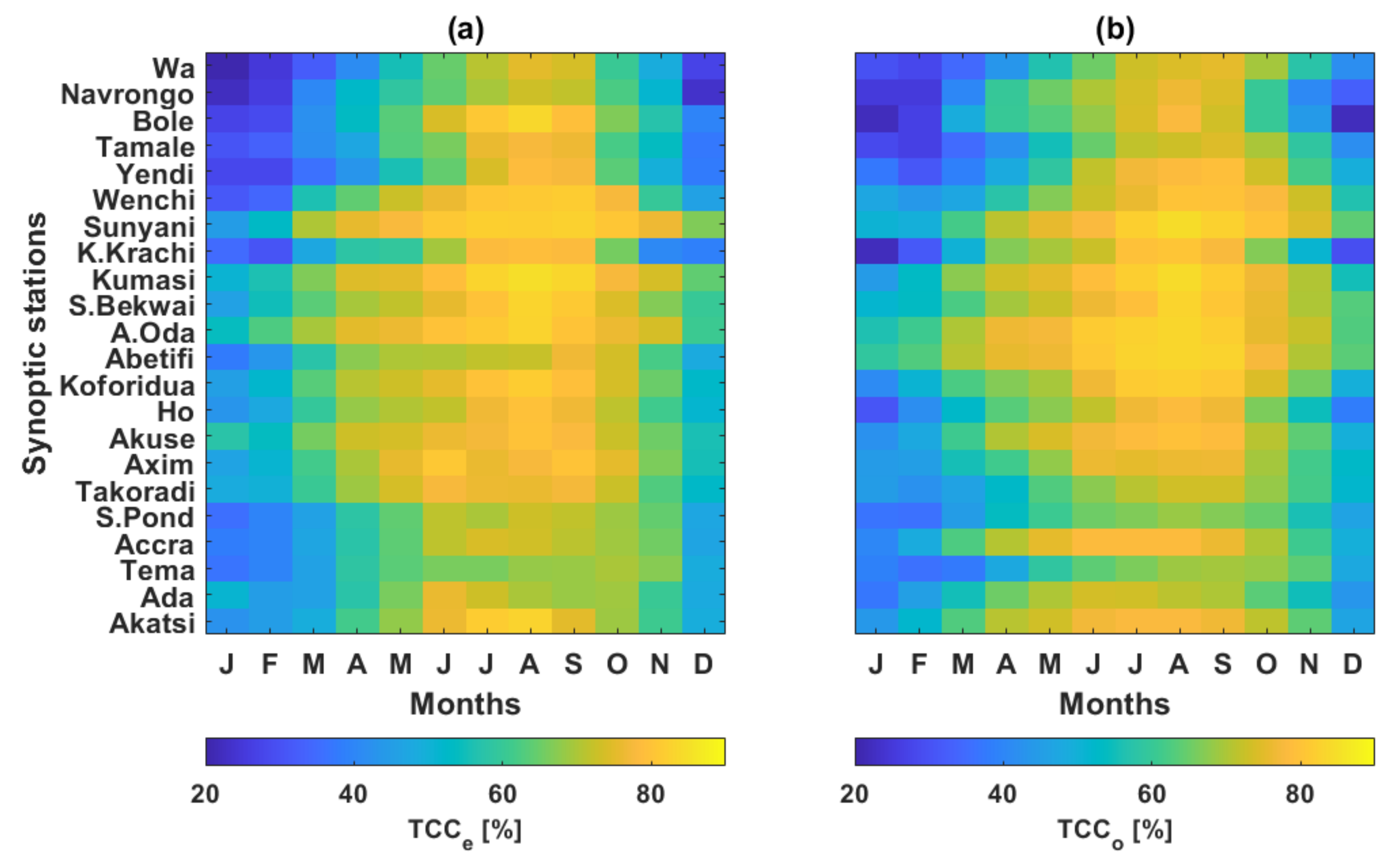
3.1. Performance of Empirical Cloud Cover Estimation and Bias Correction

From the empirical estimation and bias correction described in Section 2.3, a new estimated and improved dataset of total cloud cover was developed. Figure 2 shows the results of the total cloud cover (TCC_e) bias-corrected by cumulative distribution function (CDF) matching. In principle, we adjusted the CDF of the monthly mean estimated data over the study period in accordance with the CDF of monthly mean station observed data, to minimize their difference thus ensuring our estimation was as close as possible to the observations. On the overall, a mean estimation bias of 0.002 ± 2.2% was reduced to −3.2 × 10⁻¹⁴ ± 2.3%, suggesting slight overestimations, while the coefficient of determination increased from 0.5 to 0.84.

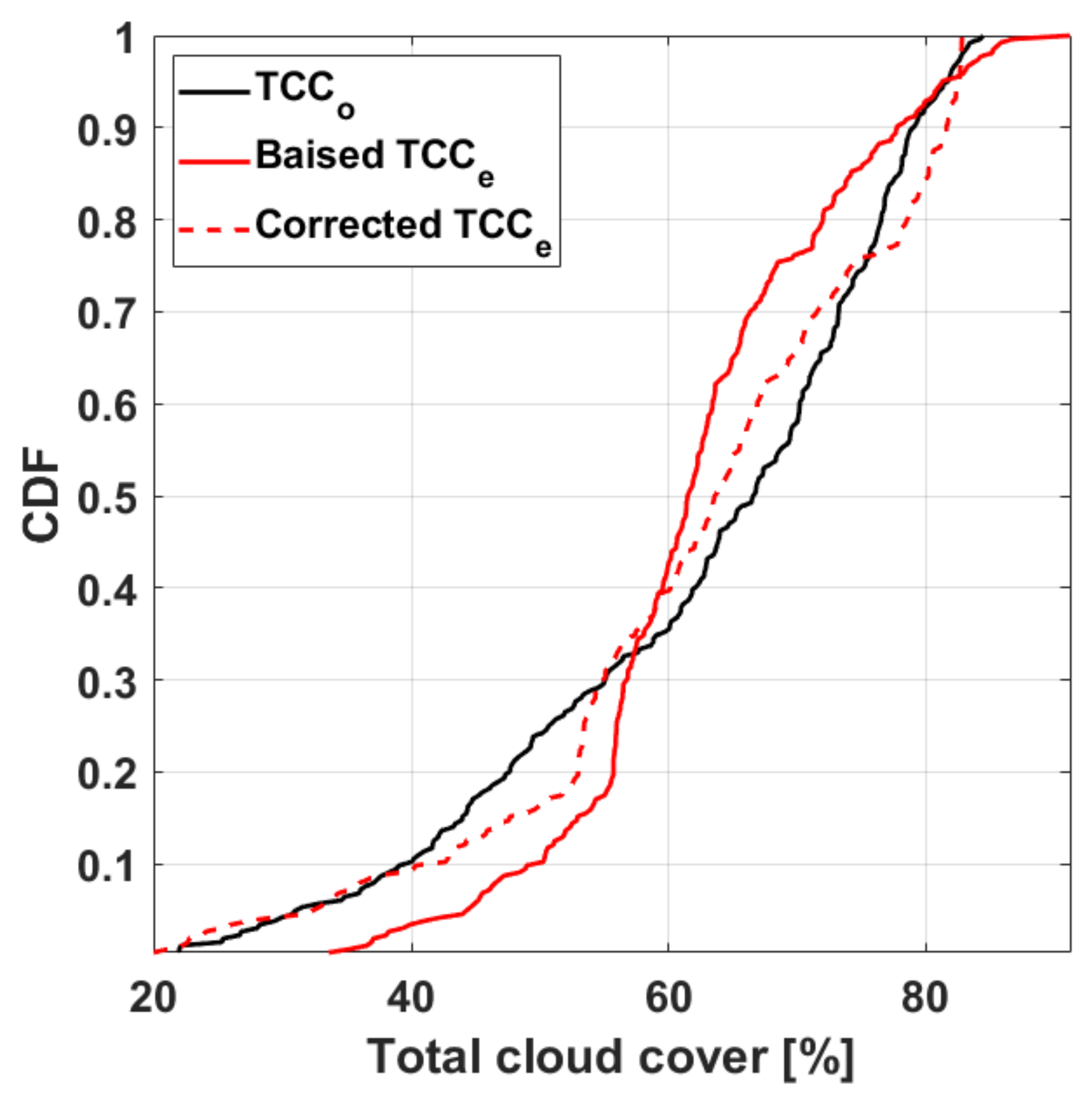
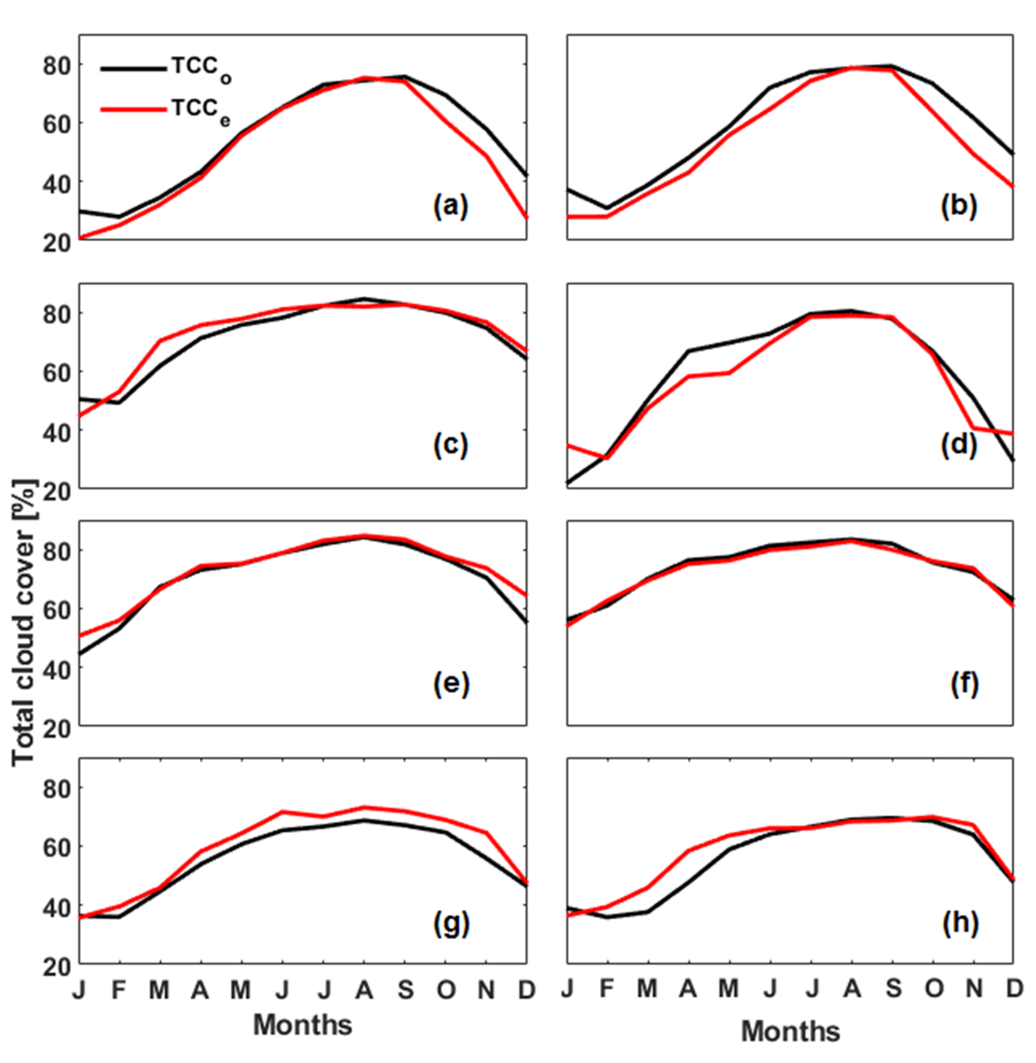
3.2. Total Cloud Cover Distribution: Comparison of Estimated and Observed

Figure 3a,b compares the spatiotemporal patterns of estimated total cloud cover (TCC_e) and station-observed total cloud cover (TCC_o) respectively. Remarkable zonal and seasonal similarities were noticed. Generally, TCC_e percentage ranges were 21–85 ± 4%, while TCC_o percentage ranges were 22–84 ± 4%. On a seasonal scale, monthly average cloud cover increased from March—when the wet monsoon commenced—and peaked during June–July–August (JJA) to September–October–November (SON) when TCC_e and TCC_o reached 82 ± 4% and 82 ± 5% respectively, whereas minimum TCC_e and TCC_o of 24 ± 10% and 23 ± 10% respectively occurred during DJF. Additionally, on the zonal scale, peak cloud cover was prevalent over the mid-southern forest-type climate regions, ranging from 37–81 ± 11% to 40–81 ± 12% for the estimated and observed datasets, while the northern savannah experienced relatively lower monthly average cloud cover of 25–77 ± 18% and 27 −76 ± 18% for estimated and observed datasets, respectively. Both datasets—modelled and human observation—agree with the cloud climatology of the southern West African sub-region presented by Danso et al. [31] and Hill et al. [4], using satellite and reanalysis products retrieved from the Clouds and the Earth’s Radiant Energy System (CERES) and ERA5 datasets. They showed that the southernmost part of West Africa—herein the forest climate zone—is the cloudiest region, with monthly mean total cloud cover reaching 70–80%. Furthermore, in a recent publication, Asilevi Junior et al. [32] presented a comprehensive statistical comparison of human observation for the present study area and cloud cover products retrieved from the National Aeronautics and Space Administration—Prediction of Worldwide Energy Resource (NASA—POWER) agro-climatological archives. They showed good agreement with mean percentage deviation of 7.8 ± 1.7, and indices of agreement between 0.7–0.99 ± 0.01, indicating strong zonal and seasonal similarities.

Despite the similarities, a few overestimations and underestimations can be noticed. For example, a mean 1–3% underestimation was seen over the northern area comprising the savannah and transitional climate zones (see Figure 3a), whereas the southern cloud cover was variously overestimated and underestimated by ±1%. Seasonally, a mean overestimation of 2% was realized mainly during June through to November, while the December–January–February (DJF) season was largely underestimated, most prominently for stations in the savannah region. Overall, estimated and observed datasets showed reasonably good spatiotemporal agreements and can be seen as complimentary in many respects.

Figure 4 shows monthly mean time series plots comparing TCC_e and TCC_o for selected stations in the savannah region (Figure 4a,b), the transitional region (Figure 4c,d), the forest region (Figure 4e,f), and the coastal region (Figure 4g,h). Generally, all time series showed similar patterns, except for slight deviations most prominent for Takoradi (Figure 4g) and also apparent for Yendi (Figure 4b). Despite this, the best estimation for most stations was for peak cloud cover mainly during the JJA to SON seasons, while the poorest estimations were for the DJF seasons, with slight overestimations and underestimations at different stations. The challenge associated with estimating cloud cover for the DJF season can be attributed to the simplicity of the empirical equations used, which were built only on sunshine duration. Considering the close association of clouds and aerosols, and their attenuating effect on sunlight, the presupposition of clouds as the main determinant of sunshine amount is a rather coarse generalization, and may be expected to yield such deviations. This was the case during the DJF season for the study area, known as the dry Harmattan season, characterized by a countrywide dust-laden atmosphere owing to the influx of dust-carrying northeasterly winds [9,33,34].

Cloud amount was lowest during this season, with little to no precipitation, yet with slightly reduced daytime surface temperatures typically reaching 12 °C in parts of the northern savannah [31,32]. Thus, the interplay of cloud–aerosol–sunlight during this season presented a rather complex situation which might not have been well parametrized using only sunshine hours as an indicator. It is clear that different climate zones and seasons should yield different estimation performances. For example, Zhu et al. [20] revealed that the performance of estimating sunshine duration from satellite-derived cloud cover data was variable for different seasons; their results showed R² = 0.93, 0.96, 0.93, and 0.89 for spring, summer, autumn, and winter, respectively. Meanwhile, slight deviations were also associated with the wet monsoon period, which may be attributed to the general complexity of cloud dynamics and climatology over the area.

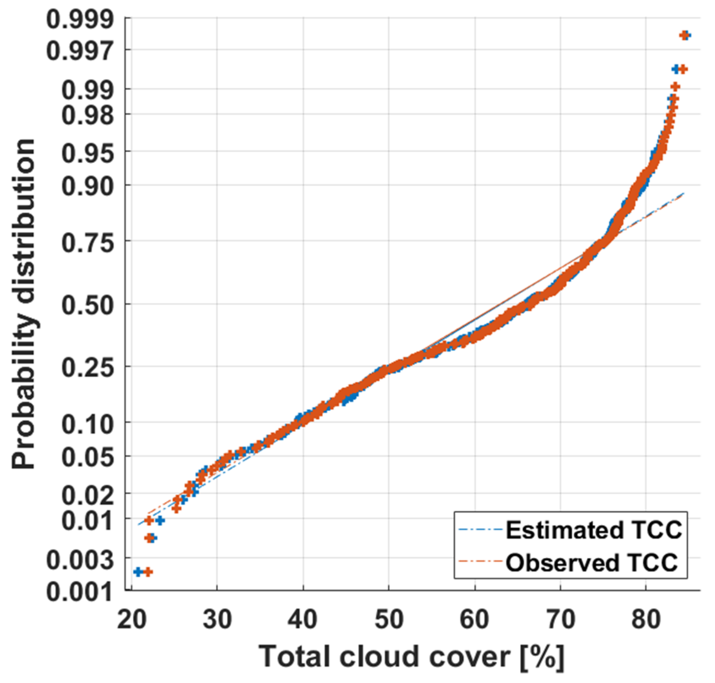
3.3. Statistical Evaluation of Cloud Cover Estimation

To assess and quantify the performance of estimation, various statistical methods described in Section 2.4 are presented. Figure 5a shows a color plot representing the space and time variations in the residual error (RE) between estimated and observed total cloud cover. The RE between TCC_e and TCC_o datasets varied between −18–21 ± 2%, with 64% −5 ≤ RE ≤ 5, and 35% −2 ≤ RE ≤ 2. Also, 47% positive REs and 53% negative REs were indicative of slight overestimations. The lowest RE was in the transition region towards the south, during the March–April–May (MAM) season, while the highest was over the northern area, largely during the DJF season.

Additionally, the control chart in Figure 5b shows that 64% of the monthly mean REs for each observation site agreed with the standard deviation of ±4%, 9% were on the standard deviation limit, and 27% were out of standard deviation range. This further indicates the close resemblance of estimated measurements to the observed, despite the −18–21 ± 2% RE range. In general, the estimations were in a reasonable range, and accurately described the cloud climatology of the study area as presented by several authors [4,32].

For further analysis,

Table 2. Summary of statistical indices comparing estimated and observed total cloud cover for all stations in the four climate zones. Root mean square error (RMSE), mean bias error (MBE), and Pearson’s correlation coefficient (r).

Stations	RMSE	MBE	r
Wa	4.66	2.39	0.97
Navrongo	4.19	1.30	0.96
Bole	5.93	−2.49	0.94
Tamale	3.89	−1.07	0.96
Yendi	5.07	3.06	0.98
Wenchi	6.11	0.81	0.90
Sunyani	2.76	−0.84	0.96
Kete Krachi	5.07	0.78	0.95
Kumasi	2.60	−1.20	0.98
Sefwi Bekwai	1.62	0.51	0.98
Oda	1.08	0.42	0.99
Abetifi	9.14	6.15	0.96
Koforidua	1.76	−0.51	0.99
Ho	4.83	−2.69	0.99
Akuse	4.01	−1.59	0.97
Axim	3.77	−2.45	0.98
Takoradi	6.17	−3.69	0.90
Salt Pond	3.24	−2.02	0.99
Accra	5.90	3.24	0.91
Tema	3.32	−1.37	0.96
Ada	4.49	−0.32	0.87
Akatsi	4.38	1.60	0.93

summarizes additional statistical indices used in the comparisons. Overall, RMSE = 1.1–9.1 ± 1.8%, MBE = −3.7–6.1 ± 2.3%, and Pearson’s correlation coefficients (r) = 0.87–0.99 ± 0.03, for all synoptic stations.

In the respective order of savannah, transition, forest, and coastal zones, the mean RMSE = 4.75, 4.65, 3.82, and 4.52, MBE = 0.64, 0.25, −0.71, and 0.79, and r = 0.96, 0.93, 0.97, and 0.92, depicting generally good correlations and moderate deviations.

Finally, an interesting statistical feature worth exploring is the probability distribution in the TCC_e/TCC_o pairwise datasets, depicted in a normal probability plot in Figure 6. It can be seen that estimated and observed cloud cover probability distribution were both asymmetrically left-skewed, as data occurrences did not align with the hypothetical normal line based on the data distribution. In both datasets, for all 22 stations in all climate regions, the chance of above average TCC > 50%. Specifically, for the savannah, transition, forest, and coastal climate regions, TCC_o had 58%, 61%, 59%, and 60% chances of above average occurrence, respectively, while TCC_e had 55%, 58%, 60%, and 60% chances of above average occurrence, respectively. This type of distribution can be attributed to the complex and rapidly changing cloud cover characteristics over the study area. This suggests that, on a monthly average scale, higher cloud cover types are more frequent than lower cloud cover types, which may have relevant application in weather forecasting and energy meteorology [1].

4. Conclusions

This study adopted a mechanistic approach to develop total cloud cover data from sunshine duration measurements spanning 2015–2019, in order to improve on traditional human observation, which may be subject to observer inaccuracies owing to impaired vision. First, based on the theory and hypothesis that cloud cover and sunshine amount sum up to unity, several regression methods were tested to develop empirical equations. Then, coupled with bias correction by cumulative distribution function (CDF) matching, total cloud cover was estimated from sunshine duration data derived from 22 synoptic weather stations, and compared with observations. A Matlab script—adaptable to any climate region—was developed to execute the procedure. From the results presented, the estimated percentage of total cloud cover, 20.8–84.7 ± 3.5%, compared well with station observation, 21.9–84.4 ± 3.5%, with root mean square errors of 1.08–9.13 ± 1.8% and correlation coefficients of 0.87–0.99 ± 0.03. In summary, the spatiotemporal characteristics were preserved, indicating the presence of denser clouds over the southern forest-type climate, prevalent during June–September. Moreover, modelled and observed total cloud cover showed a non-normality, indicating the prevalence of above average cloud cover percentage over the study area. The results are useful for weather prediction and application in meteorology, and thus provide a template and theoretical framework for atmospheric research and climate mitigation studies.

References

1. Mulkey, S.S.; Kitajima, K.; Wright, S.J. Plant physiological ecology of tropical forest canopies. Trends Ecol. Evol. 1996, 11, 408–412. [Google Scholar] [CrossRef]
2. Shen, L.; Zhao, C. Dominance of shortwave radiative heating in the sea-land breeze amplitude and its impacts on atmospheric visibility in Tokyo, Japan. J. Geophys. Res. Atmos. 2020, 125, e2019JD031541. [Google Scholar] [CrossRef]
3. Silva, A.A.; Souza-Echer, M.P. Ground-based observations of clouds through both an automatic imager and human observation. Meteorol. Appl. 2016, 23, 150–157. [Google Scholar] [CrossRef] [Green Version]
4. Hill, P.G.; Allan, R.P.; Chiu, J.C.; Bodas-Salcedo, A.; Knippertz, P. Quantifying the contribution of different cloud types to the radiation budget in southern West Africa. J. Clim. 2018, 31, 5273–5291. [Google Scholar] [CrossRef]
5. van der Linden, R.; Fink, A.H.; Redl, R. Satellite-based climatology of low-level continental clouds in southern West Africa during the summer monsoon season. J. Geophys. Res. Atmos. 2015, 120, 1186–1201. [Google Scholar] [CrossRef]
6. Fink, A.H.; Paeth, H.; Ermert, V.; Pohle, S.; Diederich, M. I-5.1 Meteorological processes influencing the weather and climate of Benin. Int. J. Climatol. 2010, 5, 135–149. [Google Scholar]
7. Jeppesen, J.H.; Jacobsen, R.H.; Inceoglu, F.; Toftegaard, T.S. A cloud detection algorithm for satellite imagery based on deep learning. Remote Sens. Environ. 2019, 229, 247–259. [Google Scholar] [CrossRef]
8. Rossow, W.B.; Schiffer, R.A. ISCCP cloud data products. Bull. Am. Meteorol. Soc. 1991, 72, 2–20. [Google Scholar] [CrossRef]
9. Asilevi, P.J.; Quansah, E.; Amekudzi, L.K.; Annor, T.; Klutse, N.A.B. Modeling the spatial distribution of Global Solar Radiation (GSR) over Ghana using the Ångström-Prescott sunshine duration model. Sci. Afr. 2019, 4, e00094. [Google Scholar] [CrossRef]
10. Amekudzi, L.K.; Yamba, E.I.; Preko, K.; Asare, E.O.; Aryee, J.; Baidu, M.; Codjoe, S.N. Variabilities in rainfall onset, cessation and length of rainy season for the various agro-ecological zones of Ghana. Climate 2015, 3, 416–434. [Google Scholar] [CrossRef]
11. Asante, F.A.; Amuakwa-Mensah, F. Climate change and variability in Ghana: Stocktaking. Climate 2015, 3, 78–99. [Google Scholar] [CrossRef] [Green Version]
12. Chaboureau, J.-P.; Söhne, N.; Guichard, F. Verification of Cloud Cover Forecast with Satellite Observation over West Africa. Mon. Weather Rev. 2008, 136, 4421–4434. [Google Scholar]
13. Knippertz, P.; Fink, A.H.; Schuster, R.; Trentmann, J.; Schrage, J.M.; Yorke, C. Ultra-low clouds over the southern West African monsoon region. Geophys. Res. Lett. 2011, 38, 1–7. [Google Scholar] [CrossRef] [Green Version]
14. World Meteorological Organization. WMO-NO.544—Manual on the Global Observing System; WMO: Geneva, Switzerland, 2003. [Google Scholar]
15. Baumgartner, D.J.; Pötzi, W.; Freislich, H.; Strutzmann, H.; Veronig, A.M.; Foelsche, U.; Rieder, H.E. A comparison of long-term parallel measurements of sunshine duration obtained with a Campbell-Stokes sunshine recorder and two automated sunshine sensors. Theor. Appl. Climatol. 2018, 133, 263–275. [Google Scholar] [CrossRef] [Green Version]
16. Badescu, V.; Paulescu, M. Statistical properties of the sunshine number illustrated with measurements from Timisoara (Romania). Atmos. Res. 2011, 101, 194–204. [Google Scholar] [CrossRef]
17. Neske, S. About the Relation between Sunshine Duration and Cloudiness on the Basis of Data from Hamburg. J. Sol. Energy 2014, 2014, 1–7. [Google Scholar] [CrossRef]
18. Ahamed, M.S.; Guo, H.; Tanino, K. Evaluation of a cloud cover based model for estimation of hourly global solar radiation in Western Canada. Int. J. Sustain. Energy 2019, 38, 64–73. [Google Scholar] [CrossRef]
19. Sarkar, M.N.I. Estimation of solar radiation from cloud cover data of Bangladesh. Renew. Wind Water Sol. 2016, 3, 1–15. [Google Scholar] [CrossRef] [Green Version]
20. Zhu, W.; Wu, B.; Yan, N.; Ma, Z.; Wang, L.; Liu, W.; Xing, Q.; Xu, J. Estimating sunshine duration using hourly total cloud amount data from a geostationary meteorological satellite. Atmosphere 2020, 11, 26. [Google Scholar] [CrossRef] [Green Version]
21. Michelangeli, P.A.; Vrac, M.; Loukos, H. Probabilistic downscaling approaches: Application to wind cumulative distribution functions. Geophys. Res. Lett. 2009, 36, 1–6. [Google Scholar] [CrossRef]
22. Polo, J.; Fernández-Peruchena, C.; Salamalikis, V.; Mazorra-Aguiar, L.; Turpin, M.; Martín-Pomares, L.; Kazantzidis, A.; Blanc, P.; Remund, J. Benchmarking on improvement and site-adaptation techniques for modeled solar radiation datasets. Sol. Energy 2020, 201, 469–479. [Google Scholar] [CrossRef]
23. Tahir, Z.u.R.; Asim, M.; Azhar, M.; Moeenuddin, G.; Farooq, M. Correcting solar radiation from reanalysis and analysis datasets with systematic and seasonal variations. Case Stud. Therm. Eng. 2021, 25, 100933. [Google Scholar] [CrossRef]
24. Schumann, K.; Beyer, H.G.; Chhatbar, K.; Meyer, R. Improving satellite-derived solar resource analysis with parallel ground-based measurements. In Proceedings of the ISES Solar World Congress, Kassel, Germany, 28 August–2 September 2011. [Google Scholar]
25. Brocca, L.; Hasenauer, S.; Lacava, T.; Melone, F.; Moramarco, T.; Wagner, W.; Dorigo, W.; Matgen, P.; Martínez-Fernández, J.; Llorens, P.; et al. Soil moisture estimation through ASCAT and AMSR-E sensors: An intercomparison and validation study across Europe. Remote Sens. Environ. 2011, 115, 3390–3408. [Google Scholar] [CrossRef]
26. Mahmoud, M.A.; Henderson, G.R.; Epprecht, E.K.; Woodall, W.H. Estimating the Standard Deviation in Quality-Control Applications. J. Qual. Technol. 2017, 42, 348–357. [Google Scholar] [CrossRef]
27. Kim, S.T.; Jeong, H.I.; Jin, F.F. Mean Bias in Seasonal Forecast Model and ENSO Prediction Error. Sci. Rep. 2017, 7, 6029. [Google Scholar] [CrossRef] [Green Version]
28. Chai, T.; Draxler, R.R. Root mean square error (RMSE) or mean absolute error (MAE)?—Arguments against avoiding RMSE in the literature. Geosci. Model Dev. 2014, 7, 1247–1250. [Google Scholar] [CrossRef] [Green Version]
29. Pereira, H.R.; Meschiatti, M.C.; Pires, R.C.D.M.; Blain, G.C. On the performance of three indices of agreement: An easy-to-use r-code for calculating the Willmott indices. Bragantia 2018, 77, 394–403. [Google Scholar] [CrossRef] [Green Version]
30. Kavassalis, S.C.; Murphy, J.G. Understanding ozone-meteorology correlations: A role for dry deposition. Geophys. Res. Lett. 2017, 44, 2922–2931. [Google Scholar] [CrossRef]
31. Danso, D.K.; Anquetin, S.; Diedhiou, A.; Lavaysse, C.; Kobea, A.; Touré, N.D.E. Spatio-temporal variability of cloud cover types in West Africa with satellite-based and reanalysis data. Q. J. R. Meteorol. Soc. 2019, 145, 3715–3731. [Google Scholar] [CrossRef] [Green Version]
32. Asilevi Junior, P.; Opoku, N.K.; Martey, F.; Setsoafia, E.; Ahafianyo, F.; Quansah, E.; Dogbey, F.; Amankwah, S.; Padi, M. Development of High Resolution Cloud Cover Climatology Databank Using Merged Manual and Satellite Datasets over Ghana, West Africa. Atmos. Ocean 2022, 1–14. [Google Scholar] [CrossRef]
33. File, D.J.M.; Derbile, E.K. Sunshine, temperature and wind. Int. J. Clim. Change Strateg. Manag. 2020, 12, 22–38. [Google Scholar] [CrossRef]
34. Junior, P.A.; Quansah, E.; Dogbey, F. Satellite-based estimates of photosynthetically active radiation for tropical ecosystems in Ghana—West Africa. Trop. Ecol. 2022, 1–11. [Google Scholar] [CrossRef]
Figure 1. Map of the study area showing all 22 synoptic stations distributed in four main climatological zones countrywide. Adapted from Asilevi et. al. [9].
Atmosphere 13 01265 g001
Figure 2. Improved estimation by CDF matching. The black line is the CDF of station-observed total cloud cover, the red line and red dashed line are the CDFs of estimated (biased) and corrected total cloud cover, respectively.
Atmosphere 13 01265 g002
Figure 3. Comparing the spatiotemporal distribution of monthly mean TCC derived from (a) bias corrected model prediction and (b) station observation datasets at the 22 synoptic stations across the study area.
Atmosphere 13 01265 g003
Figure 4. Time series comparing sunshine-duration-based estimated total cloud cover (TCCe) and station-observed total cloud cover (TCCo) for selected stations at (a) Wa and (b) Yendi in the savannah region, (c) Sunyani and (d) Kete-Krachi in the transitional region, (e) Kumasi and (f) Akim Oda in the forest region, and (g) Takoradi and (h) Accra in the coastal region.
Atmosphere 13 01265 g004
Figure 5. (a) Color plot depicting the climatological variations of residual errors (RE) between TCCo and TCCe, and (b) control chart depicting station-by-station variation in mean RE within the lower control limit (LCL) and upper control limit (UCL) of the standard deviation of RE.
Atmosphere 13 01265 g005
Figure 6. Comparison of probability plots for normal distribution in estimated and observed total cloud cover occurrence for all climatic zones in the study area.
Atmosphere 13 01265 g006