
Establishment of a Combined Model for Ozone Concentration Simulation with Stepwise Regression Analysis and Artificial Neural Network

Abstract
:1. Introduction
2. Methods
2.1. Study Area
2.2. Data Collection
2.3. Models
2.3.1. Stepwise Regression Model
2.3.2. Artificial Neural Network Model
2.3.3. Model Validation
3. Results and Discussion
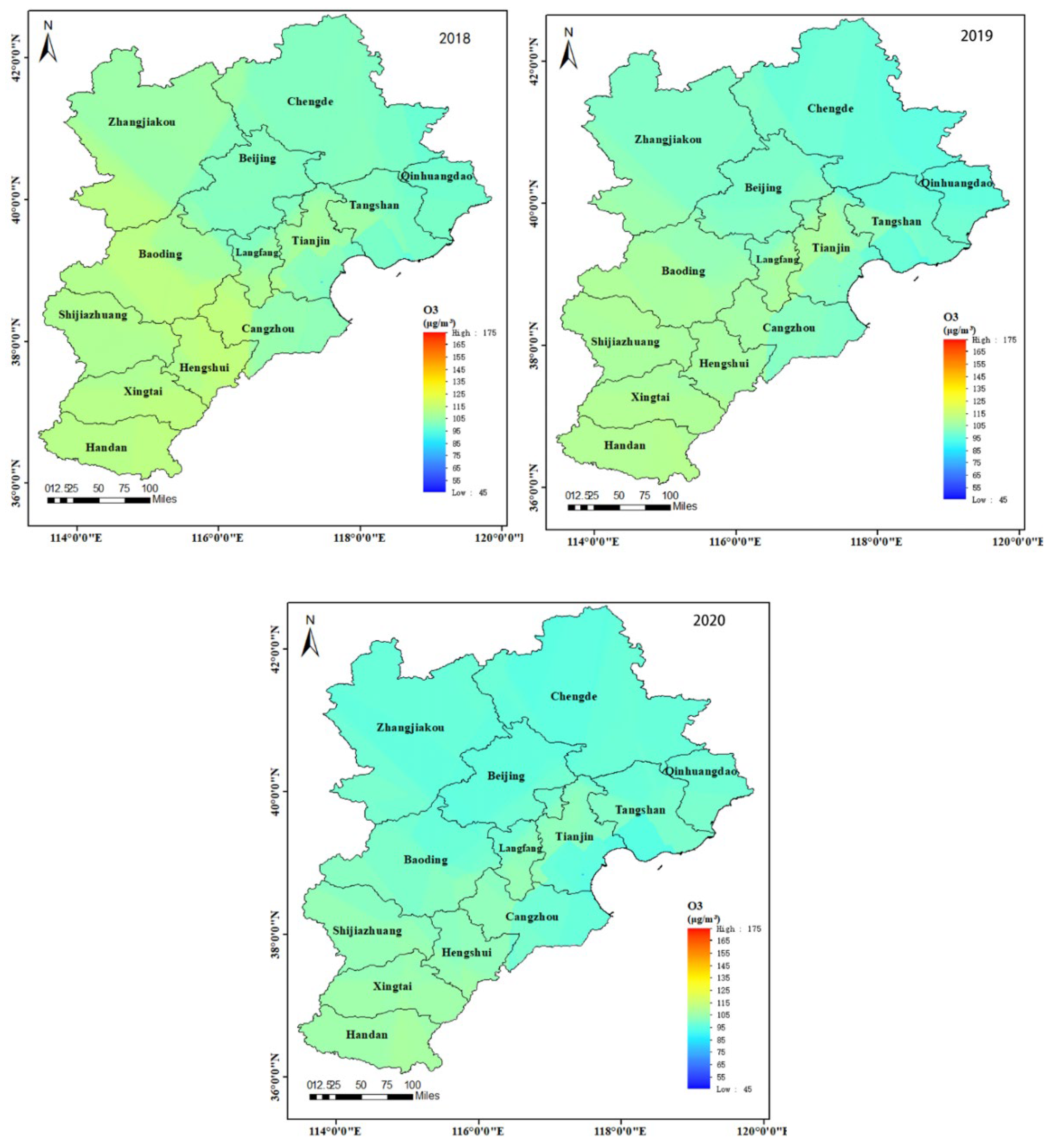
3.1. Ozone Concentration in Jing-Jin-Ji Region
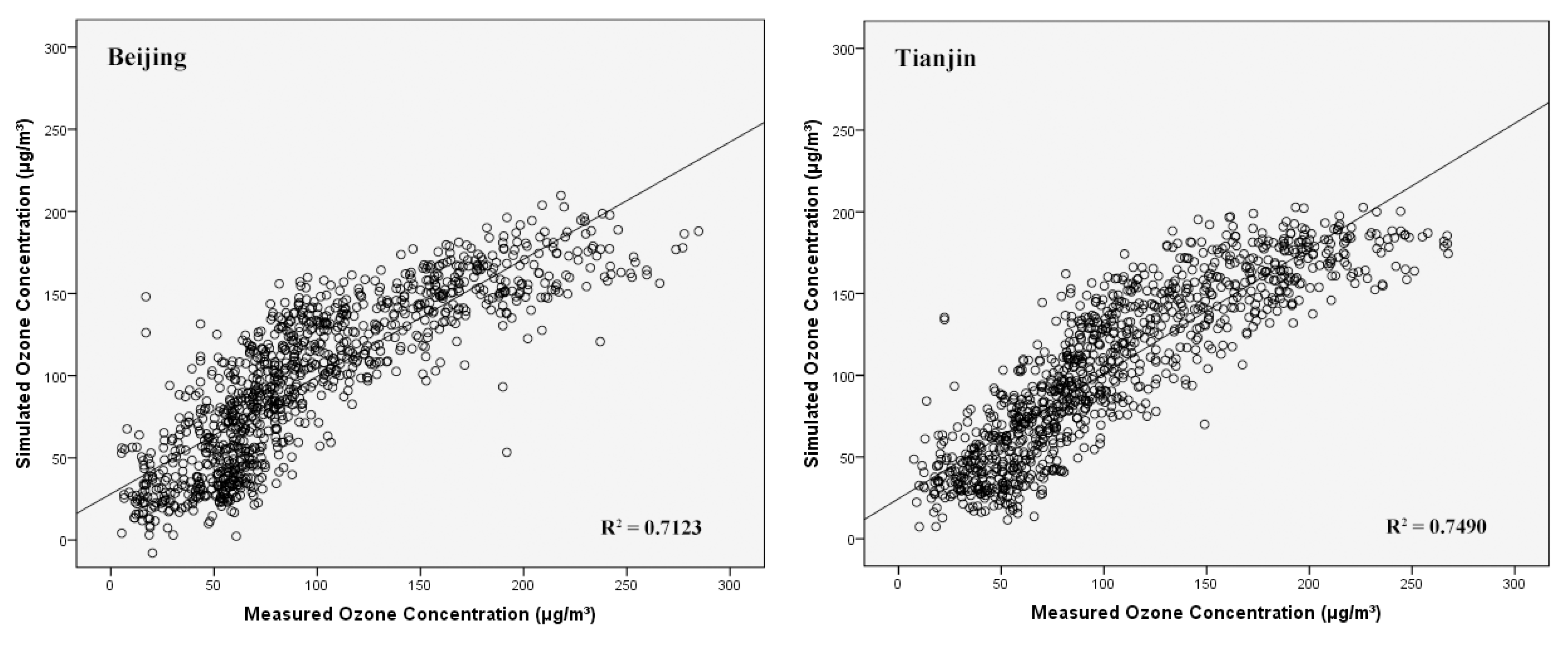
3.2. Ozone Concentration Simulated by Stepwise Regression Model
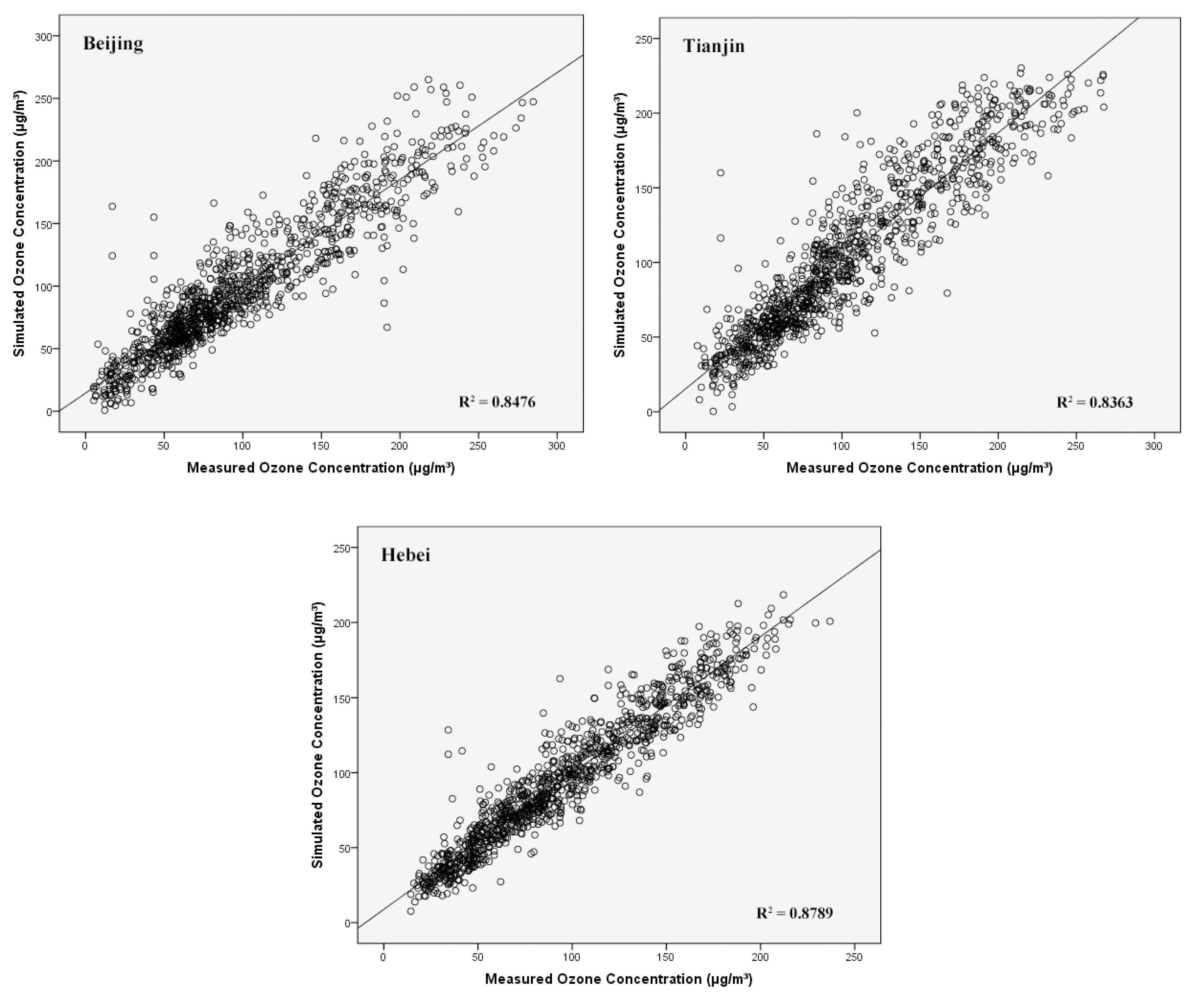
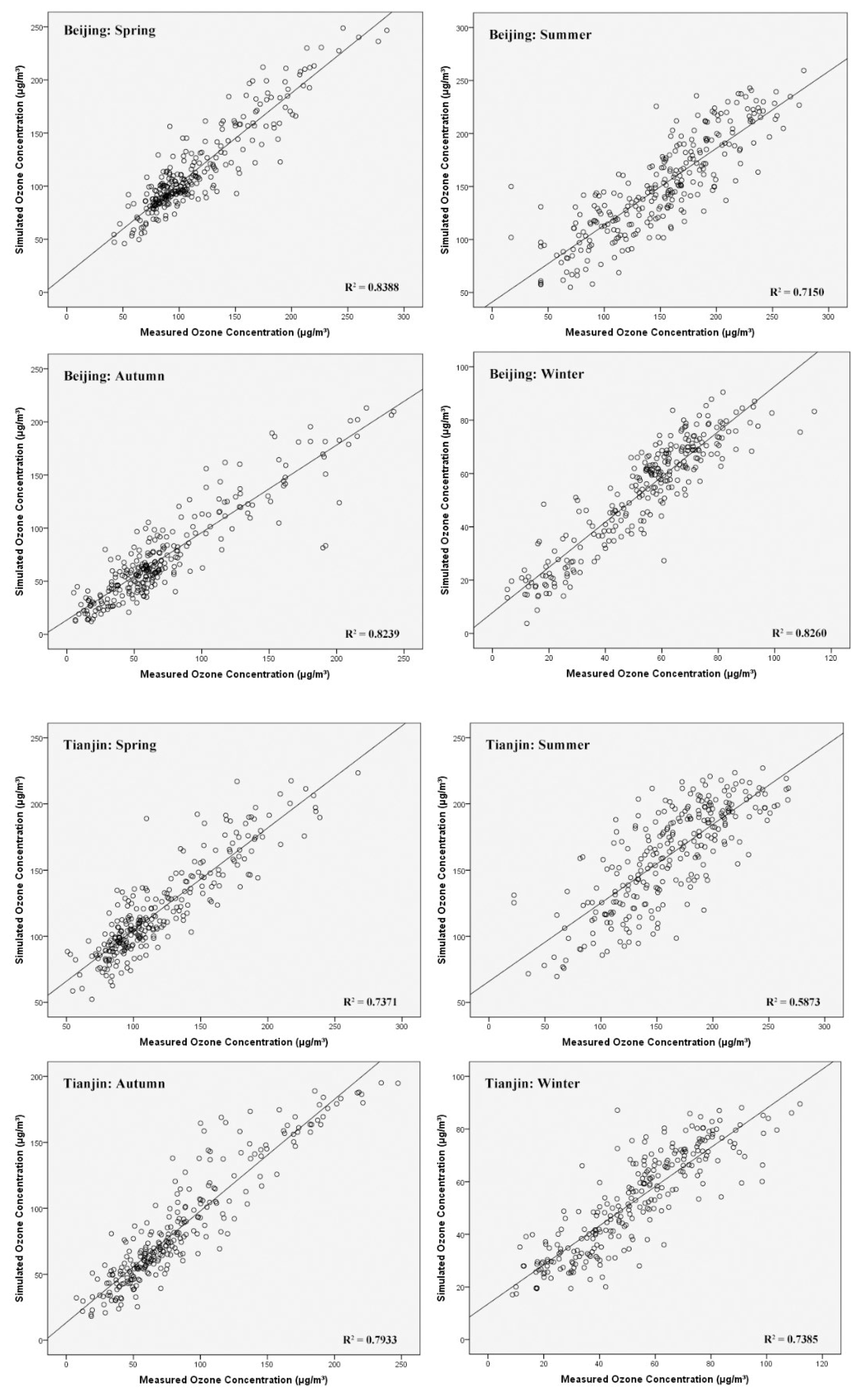
3.3. Ozone Concentration Simulated by ANN Model
3.4. Model Contrast
4. Conclusions
Supplementary Materials
Author Contributions
Funding
Data Availability Statement
Conflicts of Interest
References
- Li, X.; Li, S.; Liu, P.; Kong, Y.; Song, H. Spatial and temporal variations of ozone concentrations in China in 2016. Acta Sci. Circumstantiae 2018, 38, 1263–1274. [Google Scholar]
- Kaser, L.; Peron, A.; Graus, M.; Striednig, M.; Wohlfahrt, G.; Juráň, S.; Karl, T. Interannual variability of terpenoid emissions in an alpine city. Atmos. Chem. Phys. 2022, 22, 5603–5618. [Google Scholar] [CrossRef]
- Zeng, P.; Lyu, X.P.; Guo, H.; Cheng, H.R.; Jiang, F.; Pan, W.Z.; Wang, Z.W.; Liang, S.W.; Hu, Y.Q. Causes of ozone pollution in summer in Wuhan, Central China. Environ. Pollut. 2018, 241, 852–861. [Google Scholar] [CrossRef] [PubMed]
- Faris, H.; Alkasassbeh, M.; Rodan, A. Artificial Neural Networks for Surface Ozone Prediction: Models and Analysis. Pol. J. Environ. Stud. 2014, 23, 341–348. [Google Scholar]
- Delia, M.P.; James, D.B.; Silvia, R.S.; Anne-Marja, N.; Jarmo, K.H. Plant Volatile Organic Compounds(VOCs) in Ozone (O3) Polluted Atmospheres: The Ecological Effects. J. Chem. Ecol. 2010, 36, 22–34. [Google Scholar]
- Chan, C.K.; Yao, X. Air pollution in mega cities in China. Atmos. Environ. 2008, 42, 1–42. [Google Scholar] [CrossRef]
- Lelieveld, J.; Crutzen, P. Influences of cloud photochemical processes on tropospheric ozone. Nature 1990, 343, 227–233. [Google Scholar] [CrossRef]
- Lengyel, A.; Héberger, K.; Paksy, L.; Bánhidi, O.; Rajkó, R. Prediction of ozone concentration in ambient air using multivariate methods. Chemosphere 2004, 57, 889–896. [Google Scholar] [CrossRef]
- San José, R.; Stohl, A.; Karatzas, K.; Bohler, T.; James, P.; Pérez, J. A modelling study of an extraordinary night time ozone episode over Madrid domain. Environ. Model. Softw. 2005, 20, 587–593. [Google Scholar] [CrossRef]
- Zanis, P.; Hadjinicolaou, P.; Pozzer, A.; Tyrlis, E.; Dafka, S.; Mihalopoulos, N.; Lelieveld, J. Summertime free-tropospheric ozone pool over the eastern Mediterranean/Middle East. Atmos. Chem. Phys. 2014, 14, 115–132. [Google Scholar] [CrossRef]
- Abdul-Wahab, S.A.; Bakheit, C.S.; Al-Alawi, S.M. Principal component and multiple regression analysis in modelling of ground-level ozone and factors affecting its concentrations. Environ. Model. Softw. 2005, 20, 1263–1271. [Google Scholar] [CrossRef]
- Rajab, J.M.; MatJafri, M.; Lim, H. Combining multiple regression and principal component analysis for accurate predictions for column ozone in Peninsular Malaysia. Atmos. Environ. 2013, 71, 36–43. [Google Scholar] [CrossRef]
- Bekesiene, S.; Meidute-Kavaliauskiene, I.; Vasiliauskiene, V. Accurate prediction of concentration changes in ozone as an air pollutant by multiple linear regression and artificial neural networks. Mathematics 2021, 9, 356. [Google Scholar] [CrossRef]
- Wang, M.; Keller, J.P.; Adar, S.D.; Kim, S.-Y.; Larson, T.V.; Olives, C.; Sampson, P.D.; Sheppard, L.; Szpiro, A.A.; Vedal, S. Development of long-term spatiotemporal models for ambient ozone in six metropolitan regions of the United States: The MESA Air study. Atmos. Environ. 2015, 123, 79–87. [Google Scholar] [CrossRef]
- Al-Alawi, S.M.; Abdul-Wahab, S.A.; Bakheit, C.S. Combining principal component regression and artificial neural networks for more accurate predictions of ground-level ozone. Environ. Model. Softw. 2008, 23, 396–403. [Google Scholar] [CrossRef]
- Gao, S.; Bai, Z.; Liang, S.; Yu, H.; Chen, L.; Sun, Y.; Mao, J.; Zhang, H.; Ma, Z.; Azzi, M. Simulation of surface ozone over Hebei province, China using Kolmogorov-Zurbenko and artificial neural network (KZ-ANN) combined model. Atmos. Environ. 2021, 261, 118599. [Google Scholar] [CrossRef]
- AhmadAali, K. Liaghat, A.M. Heydari, N. Bozorg-Haddad, O. Application of artificial neural network and adaptive neural-based fuzzy inference system techniques in estimating of virtual water. Int. J. Comput. Appl. 2013, 76, 12–19. [Google Scholar]
- Sha, L.-R.; Yang, Y. In ANN-based structure optimization with fatigue reliability constrains. Appl. Mech. Mater. 2012, 204, 3128–3131. [Google Scholar] [CrossRef]
- Arsić, M.; Mihajlović, I.; Nikolić, D.; Živković, Ž.; Panić, M. Prediction of ozone concentration in ambient air using multilinear regression and the artificial neural networks methods. Ozone Sci. Eng. 2020, 42, 79–88. [Google Scholar] [CrossRef]
- Shams, S.R.; Jahani, A.; Kalantary, S.; Moeinaddini, M.; Khorasani, N. The evaluation on artificial neural networks (ANN) and multiple linear regressions (MLR) models for predicting SO2 concentration. Urban Clim. 2021, 37, 100837. [Google Scholar] [CrossRef]
- Bandyopadhyay, G.; Chattopadhyay, S. Single hidden layer artificial neural network models versus multiple linear regression model in forecasting the time series of total ozone. Int. J. Environ. Sci. Technol. 2007, 4, 141–149. [Google Scholar] [CrossRef]
- AlOmar, M.K.; Hameed, M.M.; AlSaadi, M.A. Multi hours ahead prediction of surface ozone gas concentration: Robust artificial intelligence approach. Atmos. Pollut. Res. 2020, 11, 1572–1587. [Google Scholar] [CrossRef]
- China National Environmental Monitoring Centre. China Air Quality Data (2018–2020). Available online: https://air.cnemc.cn:18007/ (accessed on 1 August 2022).
- European Centre for Medium-Range Weather Forecasts. ERA5-Land Hourly Data From 1950 to Present (2018–2020). Available online: https://cds.climate.copernicus.eu/cdsapp#!/dataset/reanalysis-era5-land?tab=form (accessed on 1 August 2022).
- Russo, A.; Lind, P.G.; Raischel, F.; Trigo, R.; Mendes, M. Neural network forecast of daily pollution concentration using optimal meteorological data at synoptic and local scales. Atmos. Pollut. Res. 2015, 6, 540–549. [Google Scholar] [CrossRef]
- Gao, M.; Yin, L.; Ning, J. Artificial neural network model for ozone concentration estimation and Monte Carlo analysis. Atmos. Environ. 2018, 184, 129–139. [Google Scholar] [CrossRef]
- Chattopadhyay, S.; Bandyopadhyay, G. Artificial neural network with backpropagation learning to predict mean monthly total ozone in Arosa, Switzerland. Int. J. Remote Sens. 2007, 28, 4471–4482. [Google Scholar] [CrossRef]
- Mekparyup, J.; Saithanu, K. Application of Artificial Neural Network Models to Predict the Ozone Concentration at the East of Thailand. Int. J. Appl. Environ. Sci. 2014, 9, 1291–1296. [Google Scholar]
- Chattopadhyay, S.; Bandyopadhyay, G. Artificial Neural Network to predict mean monthly total ozone in Arosa, Switzerland. arXiv 2006, arXiv:nlin/0608043. [Google Scholar]
- Paschalidou, A.; Iliadis, L.; Kassomenos, P.; Bezirtzoglou, C. Neural modelling of the tropospheric ozone concentrations in an urban site. In Proceedings of the 10th International Conference Engineering Applications of Neural Networks, Thessaloniki, Greece, 29–31 August 2007; pp. 436–445. [Google Scholar]
- Wang, X.; Zhao, W.; Zhang, T.; Qiu, Y.; Ma, P.; Li, L.; Wang, L.; Wang, M.; Zheng, D.; Zhao, W. Analysis of the Characteristics of Ozone Pollution in the North China Plain from 2016 to 2020. Atmosphere 2022, 13, 715. [Google Scholar] [CrossRef]
- Wang, S.; Feng, Y.P.; Cui, J.S.; Liu, D.X.; Chen, J.; Tian, L.; He, B.W.; Shen, M.Y. Spatio-temporal evolution patterns and potential source areas of ozone pollution in Shijiazhuang. Acta Sci. Circumstantiae 2020, 40, 3081–3092. [Google Scholar]
- Cui, M.; An, X.; Sun, Z.; Wang, B.; Wang, C.; Ren, W.; Li, Y. Characteristics and meteorological conditions of ozone pollution in Beijing. Ecol. Environ. Monit. Three Gorges 2019, 4, 25–35. [Google Scholar]
- Li, J. Seasonal Characteristics of Air Pollution and Weekend Effect in Shanghai. Master’s Thesis, The University of Chinese Academy of Sciences, Beijing, China, 2015. [Google Scholar]
- Juráň, S.; Šigut, L.; Holub, P.; Fares, S.; Klem, K.; Grace, J.; Urban, O. Ozone flux and ozone deposition in a mountain spruce forest are modulated by sky conditions. Sci. Total Environ. 2019, 672, 296–304. [Google Scholar] [CrossRef]
- Liu, M.-H. Analysis and Multvariate Nonlinear Prediction Model of Ground-level Ozone Time Series in Shanghai. Master’s Thesis, East China Normal University, Shanghai, China, 2009. [Google Scholar]
- Zhang, J.; Ding, W. Prediction of air pollutants concentration based on an extreme learning machine: The case of Hong Kong. Int. J. Environ. Res. Public Health 2017, 14, 114. [Google Scholar] [CrossRef]
- Zhang, W. Prediction of Ozone Concentration Based on C-PSODE Algorithm and BP Neural Network. Master’s Thesis, Zhejiang Gongshang University, Hangzhou, China, 2019. [Google Scholar]
- Xue, S.-Q. Prediction and Visualization of Air Quality Based on Error Back Propagation Neural Network Model. Master’s Thesis, Tianjin University, Tianjin, China, 2016. [Google Scholar]
- Hoshyaripour, G.; Brasseur, G.; Andrade, M.d.F.; Gavidia-Calderón, M.; Bouarar, I.; Ynoue, R.Y. Prediction of ground-level ozone concentration in São Paulo, Brazil: Deterministic versus statistic models. Atmos. Environ. 2016, 145, 365–375. [Google Scholar] [CrossRef]
- Borges, A.S.; Andrade, M.d.F.; Guardani, R. Ground-level ozone prediction using a neural network model based on meteorological variables and applied to the metropolitan area of São Paulo. Int. J. Environ. Pollut. 2012, 49, 1–15. [Google Scholar] [CrossRef]
- Feng, X.; Li, Q.; Zhu, Y.; Hou, J.; Jin, L.; Wang, J. Artificial neural networks forecasting of PM2. 5 pollution using air mass trajectory based geographic model and wavelet transformation. Atmos. Environ. 2015, 107, 118–128. [Google Scholar] [CrossRef]
- Goulier, L.; Paas, B.; Ehrnsperger, L.; Klemm, O. Modelling of urban air pollutant concentrations with artificial neural networks using novel input variables. Int. J. Environ. Res. Public Health 2020, 17, 2025. [Google Scholar] [CrossRef] [Green Version]


| City/Province | O3_8h Concentration | ||
|---|---|---|---|
| 2018 | 2019 | 2020 | |
| Beijing | 101.20 ± 58.09 | 99.77 ± 62.05 | 95.79 ± 81.52 |
| Tianjin | 106.83 ± 58.26 | 106.17 ± 62.23 | 101.16 ± 81.41 |
| Hebei | 98.64 ± 48.46 | 95.14 ± 50.19 | 95.57 ± 66.51 |
| City/Province | 2018 | 2019 | 2020 |
|---|---|---|---|
| Beijing | 64 | 72 | 54 |
| Tianjin | 83 | 81 | 58 |
| Hebei | 48 | 51 | 31 |
| City/Province | Spring | Summer | Autumn | Winter |
|---|---|---|---|---|
| Beijing | 114.45 ± 44.21 | 150.65 ± 53.72 | 72.54 ± 48.35 | 53.43 ± 21.39 |
| Tianjin | 119.63 ± 40.41 | 161.56 ± 48.58 | 83.27 ± 46.93 | 52.23 ± 21.78 |
| Hebei | 113.07 ± 32.22 | 142.08 ± 35.48 | 75.83 ± 37.86 | 50.23 ± 19.42 |
| City/Province | Model | Adjusted R2 | RMSE | MAE |
|---|---|---|---|---|
| Beijing | SR | 0.7123 | 30.89 | 23.92 |
| ANN | 0.8476 | 22.47 | 16.24 | |
| Tianjin | SR | 0.7490 | 28.84 | 22.57 |
| ANN | 0.8363 | 23.28 | 17.00 | |
| Hebei | SR | 0.8080 | 20.72 | 15.68 |
| ANN | 0.8789 | 16.46 | 11.56 |
| City/Province | Input Parameters |
|---|---|
| Beijing | T2M, SSR, WD, PM2.5, NO2, CO, BLH |
| Tianjin | T2M, SSR, WD, PM2.5, NO2, CO, BLH, WS |
| Hebei | T2M, SSR, WD, PM2.5, NO2, CO, WS, BLH, SP |
| City/Province | Activation Function | Number of Hidden Layer Nodes | Adjusted R2 | RMSE | MAE |
|---|---|---|---|---|---|
| Beijing | tanh | 3 | 0.8380 | 23.18 | 16.46 |
| 4 | 0.8519 | 22.16 | 15.75 | ||
| 5 | 0.8476 | 22.48 | 16.24 | ||
| sigmoid | 3 | 0.8294 | 23.78 | 16.95 | |
| 4 | 0.8437 | 22.76 | 16.06 | ||
| 5 | 0.8439 | 22.75 | 16.14 | ||
| Tianjin | tanh | 3 | 0.8308 | 23.68 | 17.29 |
| 4 | 0.8188 | 24.50 | 17.92 | ||
| 5 | 0.8363 | 23.28 | 17.00 | ||
| sigmoid | 3 | 0.8186 | 24.51 | 17.83 | |
| 4 | 0.8174 | 24.60 | 18.18 | ||
| 5 | 0.8332 | 23.51 | 17.27 | ||
| Hebei | tanh | 3 | 0.8789 | 16.46 | 11.56 |
| 4 | 0.8817 | 16.26 | 11.17 | ||
| 5 | 0.8881 | 15.82 | 10.90 | ||
| sigmoid | 3 | 0.8752 | 16.70 | 11.76 | |
| 4 | 0.8761 | 16.65 | 11.63 | ||
| 5 | 0.8921 | 15.53 | 10.61 |
| City/Province | Season | Adjusted R2 | RMSE | MAE |
|---|---|---|---|---|
| Beijing | spring | 0.8388 | 17.53 | 12.80 |
| summer | 0.7150 | 28.31 | 22.07 | |
| autumn | 0.8239 | 20.03 | 14.10 | |
| winter | 0.8260 | 8.80 | 6.78 | |
| Tianjin | spring | 0.7371 | 20.42 | 14.07 |
| summer | 0.5873 | 30.75 | 24.22 | |
| autumn | 0.7933 | 21.02 | 14.28 | |
| winter | 0.7385 | 10.97 | 8.15 | |
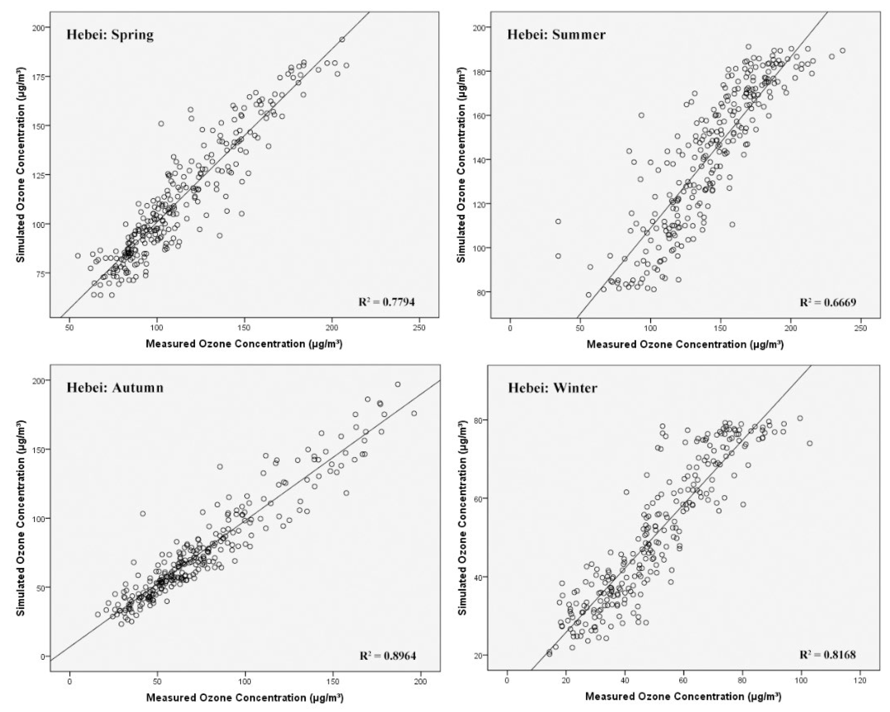
| Hebei | spring | 0.7794 | 14.88 | 9.187 |
| summer | 0.6669 | 20.14 | 13.94 | |
| autumn | 0.8964 | 11.99 | 8.66 | |
| winter | 0.8168 | 8.17 | 6.24 |
| City/Province | Model | POD | TS | FAR |
|---|---|---|---|---|
| Beijing | SR | 0.5368 | 0.4880 | 0.1570 |
| ANN | 0.7684 | 0.6697 | 0.1609 | |
| Tianjin | SR | 0.6804 | 0.5709 | 0.2199 |
| ANN | 0.8037 | 0.6692 | 0.2000 | |
| Hebei | SR | 0.3923 | 0.3566 | 0.2031 |
| ANN | 0.6846 | 0.5779 | 0.2124 |
Publisher’s Note: MDPI stays neutral with regard to jurisdictional claims in published maps and institutional affiliations. |
© 2022 by the authors. Licensee MDPI, Basel, Switzerland. This article is an open access article distributed under the terms and conditions of the Creative Commons Attribution (CC BY) license (https://creativecommons.org/licenses/by/4.0/).
Share and Cite
Yu, J.; Xu, L.; Gao, S.; Chen, L.; Sun, Y.; Mao, J.; Zhang, H. Establishment of a Combined Model for Ozone Concentration Simulation with Stepwise Regression Analysis and Artificial Neural Network. Atmosphere 2022, 13, 1371. https://doi.org/10.3390/atmos13091371
Yu J, Xu L, Gao S, Chen L, Sun Y, Mao J, Zhang H. Establishment of a Combined Model for Ozone Concentration Simulation with Stepwise Regression Analysis and Artificial Neural Network. Atmosphere. 2022; 13(9):1371. https://doi.org/10.3390/atmos13091371
Chicago/Turabian StyleYu, Jie, Lingxuan Xu, Shuang Gao, Li Chen, Yanling Sun, Jian Mao, and Hui Zhang. 2022. "Establishment of a Combined Model for Ozone Concentration Simulation with Stepwise Regression Analysis and Artificial Neural Network" Atmosphere 13, no. 9: 1371. https://doi.org/10.3390/atmos13091371