Retrieved XCO2 Accuracy Improvement by Reducing Aerosol-Induced Bias for China’s Future High-Precision Greenhouse Gases Monitoring Satellite Mission


Abstract
:1. Introduction
2. Materials and Methods
2.1. Basic Configuration of HGMS
2.2. Radiance Simulation for HGMS
2.3. XCO2 and AOD Datasets for HGMS
2.3.1. Data Screening and Fusion
2.3.2. Data Segmentation
3. Results and Discussion
3.1. Radiance Simulation Analysis
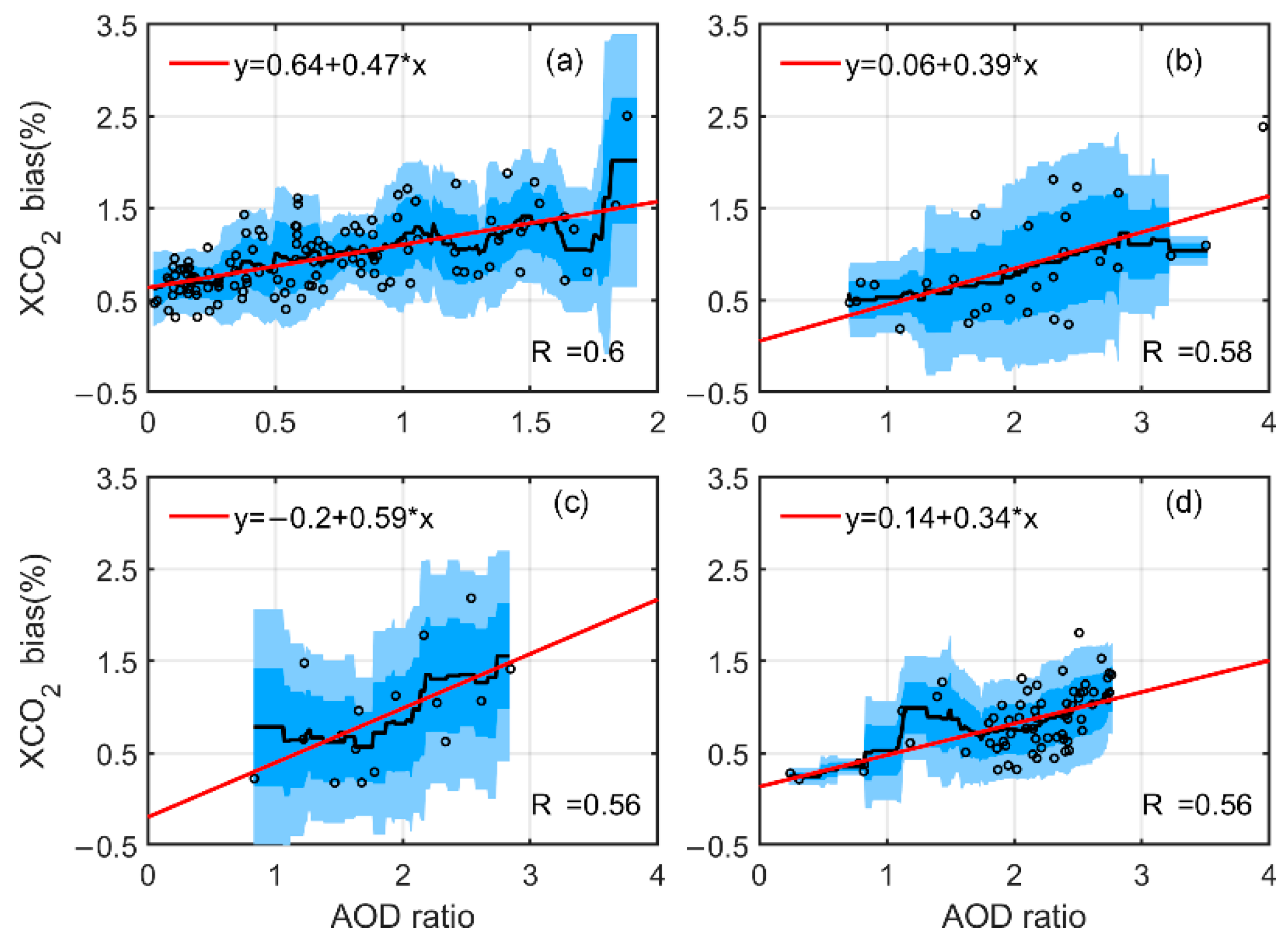
3.2. Correlation Analysis
3.3. Validation
3.4. Discussion
4. Conclusions
Author Contributions
Funding
Institutional Review Board Statement
Informed Consent Statement
Data Availability Statement
Acknowledgments
Conflicts of Interest
Appendix A

Appendix B

| Site (Location) | Date | |||
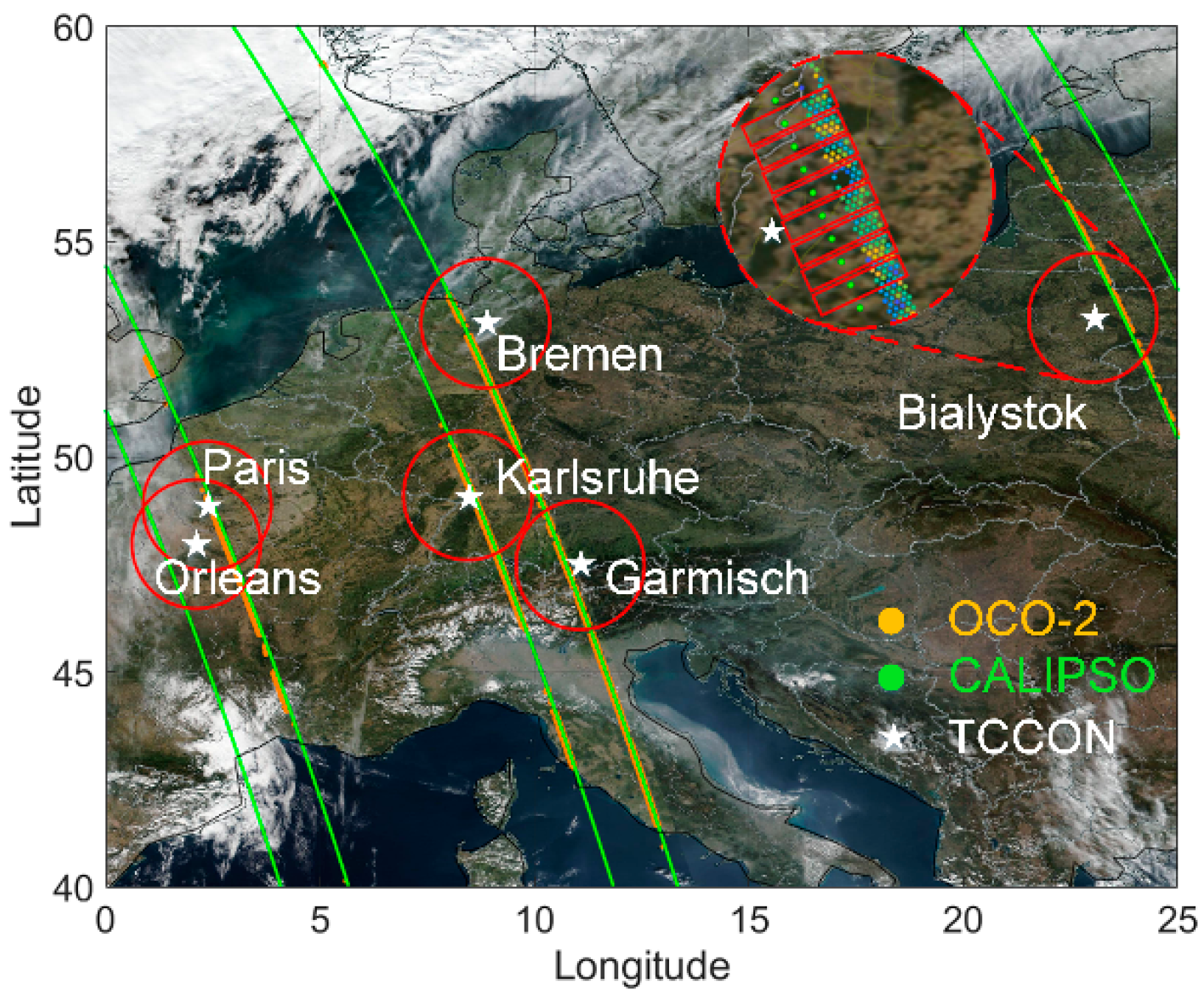
| Bialystok (53.23° N, 23.025° E) | 26 Feb 2015 23 Mar 2015 25 Mar 2015 30 Mar 2015 12 May 2015 11 Jun 2015 13 Jun 2015 6 Jul 2015 | 20 Jul 2015 31 Jul 2015 1 Sep 2015 22 Sep 2015 10 Oct 2015 25 Nov 2015 18 Mar 2016 25 Mar 2016 | 19 Apr 2016 26 Apr 2016 3 May 2016 21 May 2016 28 May 2016 4 Jun 2016 22 Jun 2016 29 Jun 2016 | 24 Jul 2016 31 Jul 2016 7 Aug 2016 1 Sep 2016 8 Sep 2016 19 Sep 2016 22 Nov 2016 29 Nov 2016 |
| Karlsruhe (49.10° N, 8.44° E) | 7 May 2015 17 Jun 2015 13 Aug 2015 21 Sep 2015 24 Nov 2015 19 Dec 2015 | 26 Dec 2015 20 Jan 2016 2 May 2016 10 Jun 2016 5 Jul 2016 7 Jul 2016 | 21 Jul 2016 30 Jul 2016 1 Aug 2016 6 Aug 2016 8 Aug 2016 31 Aug 2016 | 7 Sep 2016 14 Sep 2016 16 Oct 2016 |
| Bremen (53.10° N, 8.85° E) | 13 Aug 2015 7 Sep 2015 | 11 Apr 2016 2 May 2016 | 24 Aug 2016 31 Aug 2016 | 28 Nov 2016 |
| Garmisch (47.48° N, 11.06° E) | 18 Feb 2015 18 May 2015 10 Jun 2015 17 Jun 2015 5 Jul 2015 | 6 Aug 2015 13 Aug 2015 21 Sep 2015 10 Nov 2015 24 Nov 2015 | 20 May 2016 28 Jun 2016 5 Jul 2016 31 Aug 2016 7 Sep 2016 | 27 Oct 2016 3 Nov 2016 |
| Orleans (47.97° N, 2.113° E) | 21 Feb 2015 23 Mar 2015 25 Mar 2015 1 Apr 2015 10 May 2015 19 May 2015 21 May 2015 13 Jun 2015 15 Jul 2015 | 22 Jul 2015 29 Jul 2015 10 Sep 2015 24 Sep 2015 12 Oct 2015 19 Oct 2015 26 Oct 2015 4 Dec 2015 22 Dec 2015 | 20 Mar 2016 27 Mar 2016 10 Apr 2016 28 Apr 2016 5 May 2016 6 Jun 2016 24 Jun 2016 8 Jul 2016 15 Jul 2016 | 9 Aug 2016 27 Aug 2016 3 Sep 2016 10 Sep 2016 28 Sep 2016 19 Oct 2016 30 Oct 2016 6 Nov 2016 |
| Paris (48.846° N, 2.356° E) | 12 May 2015 21 May 2015 15 Jul 2015 | 10 Sep 2015 24 Sep 2015 26 Oct 2015 | 24 Jun 2016 10 Sep 2016 28 Sep 2016 | |
References
- Liu, Y.; Wang, J.; Che, K.; Cai, Z.; Yang, D.; Wu, l. Satellite remote sensing of greenhouse gases: Progress and trends. Natl. Remote Sens. Bull. 2021, 25, 53–64. [Google Scholar] [CrossRef]
- Han, G.; Ma, X.; Liang, A.; Zhang, T.; Zhao, Y.; Zhang, M.; Gong, W. Performance Evaluation for China’s Planned CO2-IPDA. Remote Sens. 2017, 9, 768. [Google Scholar] [CrossRef]
- Wang, N.; Zhang, K.; Shen, X.; Wang, Y.; Li, J.; Li, C.; Mao, J.; Malinka, A.; Zhao, C.; Russell, L.M.; et al. Dual-field-of-view high-spectral-resolution lidar: Simultaneous profiling of aerosol and water cloud to study aerosol-cloud interaction. Proc. Natl. Acad. Sci. USA 2022, 119, e2110756119. [Google Scholar] [CrossRef] [PubMed]
- Hostetler, C.A.; Lee, K.-P.; Ferrare, R.A.; Trepte, C.R.; Hu, Y.; Vaughan, M.A.; Winker, D.M.; Omar, A.H.; Kittaka, C.; Rogers, R.R.; et al. The CALIPSO Automated Aerosol Classification and Lidar Ratio Selection Algorithm. J. Atmos. Ocean. Technol. 2009, 26, 1994–2014. [Google Scholar] [CrossRef]
- Friedlingstein, P.; Cox, P.; Betts, R.; Bopp, L.; Von Bloh, W.; Brovkin, V.; Cadule, P.; Doney, S.; Eby, M.; Fung, I.; et al. Climate-carbon cycle feedback analysis: Results from the (CMIP)-M-4 model intercomparison. J. Clim. 2006, 19, 3337–3353. [Google Scholar] [CrossRef]
- Chen, S.; Wang, S.; Su, L.; Dong, C.; Ke, J.; Zheng, Z.; Cheng, C.; Tong, B.; Liu, D. Optimization of the OCO-2 Cloud Screening Algorithm and Evaluation against MODIS and TCCON Measurements over Land Surfaces in Europe and Japan. Adv. Atmos. Sci. 2020, 37, 387–398. [Google Scholar] [CrossRef]
- Guerlet, S.; Butz, A.; Schepers, D.; Basu, S.; Hasekamp, O.P.; Kuze, A.; Yokota, T.; Blavier, J.F.; Deutscher, N.M.; Griffith, D.W.T.; et al. Impact of aerosol and thin cirrus on retrieving and validating XCO2 from GOSAT shortwave infrared measurements. J. Geophys. Res. Atmos. 2013, 118, 4887–4905. [Google Scholar] [CrossRef]
- Mao, J.; Kawa, S.R. Sensitivity studies for space-based measurement of atmospheric total column carbon dioxide by reflected sunlight. Appl. Opt. 2004, 43, 914–927. [Google Scholar] [CrossRef]
- O’Dell, C.W.; Connor, B.; Boesch, H.; O’Brien, D.; Frankenberg, C.; Castano, R.; Christi, M.; Crisp, D.; Eldering, A.; Fisher, B.; et al. The ACOS CO2 retrieval algorithm—Part 1: Description and validation against synthetic observations. Atmos. Meas. Tech. 2012, 5, 99–121. [Google Scholar] [CrossRef]
- Wunch, D.; Wennberg, P.O.; Toon, G.C.; Connor, B.J.; Fisher, B.; Osterman, G.B.; Frankenberg, C.; Mandrake, L.; O’Dell, C.; Ahonen, P.; et al. A method for evaluating bias in global measurements of CO2 total columns from space. Atmos. Chem. Phys. 2011, 11, 12317–12337. [Google Scholar] [CrossRef] [Green Version]
- Yoshida, Y.; Ota, Y.; Eguchi, N.; Kikuchi, N.; Nobuta, K.; Tran, H.; Morino, I.; Yokota, T. Retrieval algorithm for CO2 and CH4 column abundances from short-wavelength infrared spectral observations by the Greenhouse gases observing satellite. Atmos. Meas. Tech. 2011, 4, 717–734. [Google Scholar] [CrossRef]
- Yoshida, Y.; Kikuchi, N.; Morino, I.; Uchino, O.; Oshchepkov, S.; Bril, A.; Saeki, T.; Schutgens, N.; Toon, G.C.; Wunch, D.; et al. Improvement of the retrieval algorithm for GOSAT SWIR XCO2 and XCH4 and their validation using TCCON data. Atmos. Meas. Tech. 2013, 6, 1533–1547. [Google Scholar] [CrossRef]
- Crisp, D.; Fisher, B.M.; O’Dell, C.; Frankenberg, C.; Basilio, R.; Boesch, H.; Brown, L.R.; Castano, R.; Connor, B.; Deutscher, N.M.; et al. The ACOS CO2 retrieval algorithm—Part II: Global X-CO2 data characterization. Atmos. Meas. Tech. 2012, 5, 687–707. [Google Scholar] [CrossRef]
- Wei, J.; Peng, Y.; Mahmood, R.; Sun, L.; Guo, J. Intercomparison in spatial distributions and temporal trends derived from multi-source satellite aerosol products. Atmos. Chem. Phys. 2019, 19, 7183–7207. [Google Scholar] [CrossRef]
- Hu, Z.; Jin, Q.; Ma, Y.; Pu, B.; Dong, W. Temporal evolution of aerosols and their extreme events in polluted Asian regions during Terra’s 20-year observations. Remote Sens. Environ. 2021, 263, 112541. [Google Scholar] [CrossRef]
- Stier, P. Limitations of passive remote sensing to constrain global cloud condensation nuclei. Atmos. Chem. Phys. 2016, 16, 6595–6607. [Google Scholar] [CrossRef]
- Christensen, M.W.; Neubauer, D.; Poulsen, C.; Thomas, G.; Grainger, R.G. Unveiling aerosol–cloud interactions—Part 1: Cloud contamination in satellite products enhances the aerosol indirect forcing estimate. Atmos. Chem. Phys. 2017, 17, 13151–13164. [Google Scholar] [CrossRef]
- O’Dell, C.W.; Eldering, A.; Wennberg, P.O.; Crisp, D.; Gunson, M.R.; Fisher, B.; Frankenberg, C.; Kiel, M.; Lindqvist, H.; Mandrake, L.; et al. Improved retrievals of carbon dioxide from Orbiting Carbon Observatory-2 with the version 8 ACOS algorithm. Atmos. Meas. Tech. 2018, 11, 6539–6576. [Google Scholar] [CrossRef]
- Zhou, M.; Dils, B.; Wang, P.; Detmers, R.; Yoshida, Y.; O’Dell, C.W.; Feist, D.G.; Velazco, V.A.; Schneider, M.; De Mazière, M. Validation of TANSO-FTS/GOSAT XCO2 and XCH4 glint mode retrievals using TCCON data from near-ocean sites. Atmos. Meas. Tech. 2016, 9, 1415–1430. [Google Scholar] [CrossRef]
- Yang, D.; Boesch, H.; Liu, Y.; Somkuti, P.; Cai, Z.; Chen, X.; Di Noia, A.; Lin, C.; Lu, N.; Lyu, D.; et al. Toward High Precision XCO2 Retrievals From TanSat Observations: Retrieval Improvement and Validation Against TCCON Measurements. J. Geophys. Res. Atmos 2020, 125, e2020JD032794. [Google Scholar] [CrossRef]
- Wunch, D.; Wennberg, P.O.; Osterman, G.; Fisher, B.; Naylor, B.; Roehl, C.M.; O’Dell, C.; Mandrake, L.; Viatte, C.; Kiel, M.; et al. Comparisons of the Orbiting Carbon Observatory-2 (OCO-2) XCO2 measurements with TCCON. Atmos. Meas. Tech. 2017, 10, 2209–2238. [Google Scholar] [CrossRef]
- Liu, D.; Zheng, Z.; Chen, W.; Wang, Z.; Li, W.; Ke, J.; Zhang, Y.; Chen, S.; Cheng, C.; Wang, S. Performance estimation of space-borne high-spectral-resolution lidar for cloud and aerosol optical properties at 532 nm. Opt. Express 2019, 27, A481–A494. [Google Scholar] [CrossRef] [PubMed]
- Ke, J.; Sun, Y.; Dong, C.; Zhang, X.; Wang, Z.; Lyu, L.; Zhu, W.; Ansmann, A.; Su, L.; Bu, L.; et al. Development of China’s first space-borne aerosol-cloud high-spectral-resolution lidar: Retrieval algorithm and airborne demonstration. PhotoniX 2022, 3, 17. [Google Scholar] [CrossRef]
- Uchino, O.; Kikuchi, N.; Sakai, T.; Morino, I.; Yoshida, Y.; Nagai, T.; Shimizu, A.; Shibata, T.; Yamazaki, A.; Uchiyama, A.; et al. Influence of aerosols and thin cirrus clouds on the GOSAT-observed CO2: A case study over Tsukuba. Atmos. Chem. Phys. 2012, 12, 3393–3404. [Google Scholar] [CrossRef]
- Taylor, T.E.; O’Dell, C.W.; Frankenberg, C.; Partain, P.T.; Cronk, H.Q.; Savtchenko, A.; Nelson, R.R.; Rosenthal, E.J.; Chang, A.Y.; Fisher, B.; et al. Orbiting Carbon Observatory-2 (OCO-2) cloud screening algorithms: Validation against collocated MODIS and CALIOP data. Atmos. Meas. Tech. 2016, 9, 973–989. [Google Scholar] [CrossRef]
- Merrelli, A.J.; Bennartz, R.; O’Dell, C. Evaluating XCO2 Retrievals from OCO-2 with CALIOP-Derived Aerosol Priors. In Agu Fall Meeting Abstracts, Proceedings of the the 2017 AGU Fall Meeting, New Orleans, LA, USA, 11–15 December 2017; American Geophysical Union: Washington, DC, USA, 2017. [Google Scholar]
- Oyafuso, F.; Payne, V.H.; Drouin, B.J.; Devi, V.M.; Benner, D.C.; Sung, K.; Yu, S.; Gordon, I.E.; Kochanov, R.; Tan, Y.; et al. High accuracy absorption coefficients for the Orbiting Carbon Observatory-2 (OCO-2) mission: Validation of updated carbon dioxide cross-sections using atmospheric spectra. J. Quant. Spectrosc. Radiat. Transf. 2017, 203, 213–223. [Google Scholar] [CrossRef]
- Powell, K.A.; Hu, Y.; Omar, A.; Vaughan, M.A.; Winker, D.M.; Liu, Z.; Hunt, W.H.; Young, S.A. Overview of the CALIPSO Mission and CALIOP Data Processing Algorithms. J. Atmos. Ocean. Technol. 2009, 26, 2310–2323. [Google Scholar] [CrossRef]
- OCO-2 Science Team; Gunson, M.; Eldering, A. OCO-2 Level 2 Geolocated XCO2 Retrievals Results, Physical Model, Retrospective Processing V10r, version 10r; Goddard Earth Sciences Data and Information Services Center: Greenbelt, MD, USA, 2020. [CrossRef]
- Deng, A.; Yu, T.; Cheng, T.; Gu, X.; Zheng, F.; Guo, H. Intercomparison of Carbon Dioxide Products Retrieved from GOSAT Short-Wavelength Infrared Spectra for Three Years (2010–2012). Atmosphere 2016, 7, 109. [Google Scholar] [CrossRef]
- Tadić, J.; Biraud, S. An Approach to Estimate Atmospheric Greenhouse Gas Total Columns Mole Fraction from Partial Column Sampling. Atmosphere 2018, 9, 247. [Google Scholar] [CrossRef] [Green Version]
- Clough, S.A.; Shephard, M.W.; Mlawer, E.J.; Delamere, J.S.; Iacono, M.J.; Cady-Pereira, K.; Boukabara, S.; Brown, P.D. Atmospheric radiative transfer modeling: A summary of the AER codes. J. Quant. Spectrosc. Radiat. Transf. 2005, 91, 233–244. [Google Scholar] [CrossRef]
- Fomin, B.; Falaleeva, V. A Polarized Atmospheric Radiative Transfer Model for Calculations of Spectra of the Stokes Parameters of Shortwave Radiation Based on the Line-by-Line and Monte Carlo Methods. Atmosphere 2012, 3, 451–467. [Google Scholar] [CrossRef]
- Stamnes, K.; Tsay, S.C.; Wiscombe, W.; Laszlo, I. DISORT, a General-Purpose Fortran Program for Discrete-Ordinate-Method Radiative Transfer in Scattering and Emitting Layered Media: Documentation of Methodology, version 1.1; NTRS: Chicago, IL, USA, 2000. [Google Scholar]
- Emde, C.; Buras-Schnell, R.; Kylling, A.; Mayer, B.; Gasteiger, J.; Hamann, U.; Kylling, J.; Richter, B.; Pause, C.; Dowling, T. The libRadtran software package for radiative transfer calculations (version 2.0.1). Geosci. Model Dev. 2016, 9, 1647–1672. [Google Scholar] [CrossRef]
- Stamnes, K.; Tsay, S.C.; Wiscombe, W.J.; Jayaweera, K. Numerically stable algorithm for discrete-ordinate-method radiative transfer in multiple scattering and emitting layered media. Appl. Opt. 1988, 27, 2502–2509. [Google Scholar] [CrossRef] [PubMed]
- Kurucz, R.L. Synthetic Infrared Spectra. In Symposium-International Astronomical Union; Cambridge University Press: Singapore, 1994; Volume 154, p. 523. [Google Scholar]
- Wang, M.; Fan, X.; Li, X.; Liu, Q.; Qu, Y. Estimation of Land Surface Albedo from MODIS and VIIRS Data: A Multi-Sensor Strategy Based on the Direct Estimation Algorithm and Statistical-Based Temporal Filter. Remote Sens. 2020, 12, 4131. [Google Scholar] [CrossRef]
- Logothetis, S.A.; Salamalikis, V.; Kazantzidis, A. Aerosol classification in Europe, Middle East, North Africa and Arabian Peninsula based on AERONET Version 3—ScienceDirect. Atmos. Res. 2020, 239, 104893. [Google Scholar] [CrossRef]
- Garofalide, S.; Postolachi, C.; Cocean, A.; Cocean, G.; Motrescu, I.; Cocean, I.; Munteanu, B.S.; Prelipceanu, M.; Gurlui, S.; Leontie, L. Saharan Dust Storm Aerosol Characterization of the Event (9 to 13 May 2020) over European AERONET Sites. Atmosphere 2022, 13, 493. [Google Scholar] [CrossRef]
- Milinevsky, G.; Miatselskaya, N.; Grytsai, A.; Danylevsky, V.; Bril, A.; Chaikovsky, A.; Yukhymchuk, Y.; Wang, Y.; Liptuga, A.; Kyslyi, V.; et al. Atmospheric Aerosol Distribution in 2016–2017 over the Eastern European Region Based on the GEOS-Chem Model. Atmosphere 2020, 11, 722. [Google Scholar] [CrossRef]
- Qiu, R.; Han, G.; Ma, X.; Xu, H.; Shi, T.; Zhang, M. A Comparison of OCO-2 SIF, MODIS GPP, and GOSIF Data from Gross Primary Production (GPP) Estimation and Seasonal Cycles in North America. Remote Sens. 2020, 12, 258. [Google Scholar] [CrossRef]
- Liang, A.; Gong, W.; Han, G.; Xiang, C. Comparison of Satellite-Observed XCO2 from GOSAT, OCO-2, and Ground-Based TCCON. Remote Sens. 2017, 9, 1033. [Google Scholar] [CrossRef] [Green Version]
- Chen, X.; Liu, Y.; Yang, D.; Cai, Z.; Chen, H.; Wang, M. A Theoretical Analysis for Improving Aerosol-Induced CO2 Retrieval Uncertainties Over Land Based on TanSat Nadir Observations Under Clear Sky Conditions. Remote Sens. 2019, 11, 1061. [Google Scholar] [CrossRef]
- Aben, I.; Hasekamp, O.; Hartmann, W. Uncertainties in the space-based measurements of CO2 columns due to scattering in the Earth’s atmosphere. J. Quant. Spectrosc. Radiat. Transf. 2007, 104, 450–459. [Google Scholar] [CrossRef]
- Crisp, D.; Atlas, R.M.; Breon, F.M.; Brown, L.R.; Burrows, J.P.; Ciais, P.; Connor, B.J.; Doney, S.C.; Fung, I.Y.; Jacob, D.J.; et al. The Orbiting Carbon Observatory (OCO) mission. Adv. Space Res. 2004, 34, 700–709. [Google Scholar] [CrossRef]
- Amiridis, V.; Marinou, E.; Tsekeri, A.; Wandinger, U.; Schwarz, A.; Giannakaki, E.; Mamouri, R.; Kokkalis, P.; Binietoglou, I.; Solomos, S.; et al. LIVAS: A 3-D multi-wavelength aerosol/cloud database based on CALIPSO and EARLINET. Atmos. Chem. Phys. 2015, 15, 7127–7153. [Google Scholar] [CrossRef]
- Holben, B.N.; Tanré, D.; Smirnov, A.; Eck, T.F.; Slutsker, I.; Abuhassan, N.; Newcomb, W.W.; Schafer, J.S.; Chatenet, B.; Lavenu, F.; et al. An emerging ground-based aerosol climatology: Aerosol optical depth from AERONET. J. Geophys. Res. Atmos. 2001, 106, 12067–12097. [Google Scholar] [CrossRef]
- Russell, P.B.; Swissler, T.J.; McCormick, M.P. Methodology for error analysis and simulation of lidar aerosol measurements. Appl. Opt. 1979, 18, 3783–3797. [Google Scholar] [CrossRef] [PubMed]
- Schaaf, C.; Wang, Z. MCD43C3 MODIS/Terra+Aqua BRDF/Albedo Albedo Daily L3 Global 0.05Deg CMG V006, version 6; NASA EOSDIS Land Processes DAAC: Sioux Falls, SD, USA, 2015. [CrossRef]
- Wunch, D.; Toon, G.C.; Blavier, J.; Washenfelder, R.A.; Notholt, J.; Connor, B.J.; Griffith, D.; Sherlock, V.; Wennberg, P.O. The Total Carbon Column Observing Network. Philos. Trans. R. Soc. A Math. Phys. Eng. Sci. 2011, 369, 2087–2112. [Google Scholar] [CrossRef] [Green Version]


| ACHSRL | GGM | ||
|---|---|---|---|
| Parameter | Value | Parameter | Value |
| Laser wavelength | 532/1064 nm | Spectral range | 0.753–0.768/1.595–1.625/ 2.04–2.08/2.275–2.325 μm |
| Pulse energy | 150/110 mJ | ||
| Frequency | 20 Hz | Spectral resolution | <0.04/0.07/0.09/0.1 nm |
| Laser bandwidth | <100 MHz | Signal-to-noise ratio | >350/340/230/200 |
| Filter bandwidth | <2 GHz | Spatial resolution | <3 km |
| Divergence angle | 0.1 mrad | Swath | >100 km |
| Field of view | 0.2 mrad | ||
| Instrument | Product Name | Parameters | |
|---|---|---|---|
| XCO2 | OCO-2 | L2 Standard V10r | XCO2 |
| L2 Lite FP V10r | Bias corrected XCO2 | ||
| TCCON | GGG2014 | XCO2 | |
| Aerosol | OCO-2 | L2 Standard V10r | Aerosol parameters at 755 nm |
| CALIOP | L2 5km A/CPro V4-20 | Extinction coefficient at 532 nm | |
| CAD score |
| Parameters | Value |
|---|---|
| CO2 level | 360 ppm |
| Atmosphere profiles | 1976 U.S. Standard Atmosphere |
| Lambertian surface reflectance | 0.2 |
| Solar zenith angle | 32° |
| Satellite viewing angle | nadir |
| Solar irradiance spectrum | Kurucz compilation |
| Spectral band range | 6300–6400 cm−1 |
| Aerosol | Single Scattering Albedo | Asymmetry | Visibility/km |
|---|---|---|---|
| Marine | 0.98 | 0.72 | 23 |
| Rural | 0.81 | 0.64 | 5 |
| Urban | 0.52 | 0.63 | 5 |
| Site | Season | τ532 = 0 | (0, 0.1] | (0.1, 0.3] | (0.3, ∞) | NHC/NDA | Data Utilization |
|---|---|---|---|---|---|---|---|
| Bialystok | DJF | LD | LD | 0.62 | LD | 17/18 | 94.4% |
| MAM | LC | LC | 0.56 | 0.58 | 95/199 | 47.7% | |
| JJA | 0.56 | 0.62 | LC | 0.64 | 221/285 | 77.5% | |
| SON | LC | 0.61 | LC | LC | 122/275 | 44.4% | |
| Garmisch | DJF | 0.63 | LD | LD | LD | 50/50 | 100% |
| MAM | LD | 0.57 | LC | LD | 29/39 | 74.5% | |
| JJA | 0.58 | LC | 0.56 | 0.69 | 192/267 | 71.9% | |
| SON | LC | LC | LC | LC | 0/281 | 0 | |
| Karlsruhe | DJF | 0.58 | LC | LD | LD | 42/94 | 44.7% |
| MAM | LC | 0.64 | LC | LD | 45/93 | 48.3% | |
| JJA | LC | 0.60 | LC | LC | 70/187 | 37.4% | |
| SON | LC | LC | 0.57 | LD | 106/253 | 41.9% | |
| Orleans | DJF | LD | LD | 0.79 | LD | 10/17 | 58.8% |
| MAM | LC | LD | 0.64 | LC | 35/129 | 27.1% | |
| JJA | 0.62 | LC | LC | 0.70 | 120/196 | 61.2% | |
| SON | 0.59 | LC | 0.64 | LD | 143/242 | 38.5% | |
| TOTAL | 1297/2625 | 49.4% | |||||
| Site | Case | b | a | Site | Case | b | a |
|---|---|---|---|---|---|---|---|
| Bialystok | JJAτ532 = 0 | 0.09 | 4.71 | Garmisch | DJFτ532 = 0 | 0.37 | 11.8 |
| JJA(0, 0.1] | 0.49 | 0.53 | JJAτ532 = 0 | 0.18 | 5.44 | ||
| SON(0, 0.1] | 0.64 | 0.47 | MAM(0, 0.1] | 0.057 | 0.39 | ||
| DJF(0.1, 0.3] | 0.76 | 0.27 | JJA(0.1, 0.3] | 0.14 | 0.34 | ||
| MAM(0.1, 0.3] | −0.20 | 0.59 | JJA(0.3, ∞) | 0.062 | 1.58 | ||
| MAM(0.3, ∞) | 0.62 | 0.90 | Orleans | JJAτ532 = 0 | 0.18 | 5.44 | |
| JJA(0.3, ∞) | 0.28 | 1.89 | SONτ532 = 0 | 0.42 | 7.91 | ||
| Karlsruhe | DJFτ532 = 0 | 0.15 | 9.98 | DJF(0.1, 0.3] | 0.41 | 1.27 | |
| MAM(0, 0.1] | 0.15 | 0.48 | MAM(0.1, 0.3] | 0.27 | 0.35 | ||
| JJA(0, 0.1] | 0.18 | 0.26 | SON(0.1, 0.3] | 0.13 | 0.52 | ||
| SON(0.1, 0.3] | 0.48 | 0.51 | JJA(0.3, ∞) | 0.30 | 1.18 |
| Site | Season | TCCON | OCO-2 Data | Optimization OCO-2 Data | ||||||
|---|---|---|---|---|---|---|---|---|---|---|
| XCO2 | Count | XCO2 | SDCO2 | R | Count | XCO2 | SDCO2 | R | ||
| Bremen | MAM | 403.82 | 17 | 400.46 | 1.67 | 0.96 | 15 | 401.99 | 1.22 | 0.98 |
| JJA | 398.53 | 155 | 397.12 | 1.90 | 106 | 398.35 | 2.09 | |||
| SON | 399.30 | 152 | 396.90 | 3.86 | 140 | 398.74 | 3.92 | |||
| Paris | MAM | 403.07 | 58 | 396.30 | 4.10 | 0.65 | 23 | 399.96 | 3.17 | 0.68 |
| JJA | 399.51 | 53 | 394.69 | 4.64 | 43 | 400.52 | 4.28 | |||
| SON | 398.67 | 97 | 392.69 | 2.36 | 97 | 397.56 | 2.02 | |||
Publisher’s Note: MDPI stays neutral with regard to jurisdictional claims in published maps and institutional affiliations. |
© 2022 by the authors. Licensee MDPI, Basel, Switzerland. This article is an open access article distributed under the terms and conditions of the Creative Commons Attribution (CC BY) license (https://creativecommons.org/licenses/by/4.0/).
Share and Cite
Ke, J.; Wang, S.; Chen, S.; Dong, C.; Sun, Y.; Liu, D. Retrieved XCO2 Accuracy Improvement by Reducing Aerosol-Induced Bias for China’s Future High-Precision Greenhouse Gases Monitoring Satellite Mission. Atmosphere 2022, 13, 1384. https://doi.org/10.3390/atmos13091384
Ke J, Wang S, Chen S, Dong C, Sun Y, Liu D. Retrieved XCO2 Accuracy Improvement by Reducing Aerosol-Induced Bias for China’s Future High-Precision Greenhouse Gases Monitoring Satellite Mission. Atmosphere. 2022; 13(9):1384. https://doi.org/10.3390/atmos13091384
Chicago/Turabian StyleKe, Ju, Shuaibo Wang, Sijie Chen, Changzhe Dong, Yingshan Sun, and Dong Liu. 2022. "Retrieved XCO2 Accuracy Improvement by Reducing Aerosol-Induced Bias for China’s Future High-Precision Greenhouse Gases Monitoring Satellite Mission" Atmosphere 13, no. 9: 1384. https://doi.org/10.3390/atmos13091384