Article

Seasonal Variation Characteristics of VOCs and Their Influences on Secondary Pollutants in Yibin, Southwest China

1
Department of Environmental Science and Engineering, Sichuan University, Chengdu 610065, China
2
Yibin Ecological Environment Monitoring Center Station, Yibin 644099, China
*
Author to whom correspondence should be addressed.
Atmosphere 2022, 13(9), 1389; https://doi.org/10.3390/atmos13091389
Submission received: 30 July 2022 / Revised: 19 August 2022 / Accepted: 22 August 2022 / Published: 30 August 2022

Abstract

:
Volatile organic compounds (VOCs) have a crucial impact on the formation of ozone and secondary organic aerosols in the near-surface atmosphere. Understanding the composition characteristics and sources of VOCs is necessary for determining effective control policies to mitigate VOCs and related secondary pollutions. We performed on-line measurements of VOC species in typical months of each season in Yibin, a fast-growing city in Sichuan Basin in China, to identify VOC seasonal characteristics, sources, and the potential for secondary pollution formation. The average mixing ratio of VOCs in Yibin was 22.3 ppbv. Five major emission sources were identified through the positive matrix factorization model, namely, gasoline vehicle, diesel vehicle, industrial manufacturing, solvent utilization, regional background, and secondary formation. Aromatics and alkenes played leading roles in the secondary formation of ozone and secondary organic aerosols. Furthermore, m/p-xylene, ethylene, and toluene were identified to be the major reactive species. Future management should consider targeting these compounds when evaluating ozone and aerosol reduction strategies. Vehicle and solvent utilization emission mitigation would be the primary and effective ways to improve air quality in the fast-developing city in this region.

1. Introduction

Volatile organic compounds (VOCs) are significant precursors to the formation of ozone and secondary organic aerosols (SOA) [1,2,3,4,5]. They contribute to the ability of atmospheric oxidation [6,7,8,9] and further impact the quality of air, thus threatening human health. Petrochemical or industrial facilities especially can spread out various VOCs, and some of them have been identified as a crucial factor to influence human health [10,11,12], including toluene, benzene, and 1,3-butadiene [13]. Due to rapid urbanization and industrialization, air pollution has been an urgent problem to handle [14,15]. In recent years, ground-level ozone (O3) and haze events have heavily bothered urban cities in China due to the abundant emissions of precursors such as VOCs and NOx, the main factors forming photochemical pollution [16,17]. Thus, a better understanding of VOCs’ sources and their impact on secondary pollutant is crucial for making effective emission control plans.
Trying to figure out VOC sources and pollution features will help to effectively control secondary pollutants, such as O3, SOA, and peroxyacetyl nitrate (PAN) [18]. Sun and his team found that urban pollution mainly originated from anthropogenic sources, which contained vehicular exhaust, vegetation emission, solvent usage, secondary formation, and biomass burning [19]. Tan studied the temporal and spatial distribution characteristics and source origins of VOCs in Chengdu, a typical city in Sichuan Basin, and gained two dominant VOC sources, which were motor vehicle exhaust and solvent utilization [20]. Research showed that in other cities of China, industrial emissions, automobile emissions, and biomass combustion emissions were considered to be the main sources of VOCs [21,22,23,24]. Except for them, the VOC reactivity was an essential factor for ambient VOCs to form secondary pollutants in large cities [25,26,27]. Different sources could spread out various characteristic VOC species; for example, propene was the dominant driver of internal combustion engines and was identified as a tracer of vehicle exhaust in Shanghai [28,29]. Research about VOCs in China mainly concentrated on economically developed areas; a few studies were implemented in Yibin city, but there was still a lack of results on the contribution of local VOCs to the formation of second pollutants. As a very fast-growing city in Sichuan province, Yibin is located in the south of Sichuan Basin, which suffers unfavorable topographic and meteorological conditions, and it is also an important sink for pollutants in Sichuan Basin [30]. With rapid economic growth, emissions from human activities are sticky problems to handle, and Yibin has become one of the most heavily polluted cities in these years. Research about VOCs in China mainly concentrated on economically developed areas and megacities, but few studies were implemented in these mid-sized cities. Therefore, our study on VOC characteristics and sources in Yibin has a certain reference value for other cities with the same pollution characteristics.
The data for this research were received from national monitoring stations for hourly VOC data, which was mainly used to figure out the basic properties and source apportionment of seasonal VOCs in Yibin. Firstly, we classified the 112 VOCs into five categories (e.g., alkanes, alkenes, aromatics, halohydrocarbons, and OVOCs), and cleared out the major species that contributed to the measurements of VOCs. Secondly, positive matrix factorization (PMF) was conducted to identify the seasonal source apportionment of VOCs, and tried to figure out the main emissions of ambient VOC mixing ratios in Yibin. Finally, domestic maximum incremental reactivity (MIR), OH reactive rates (KOH), and fractional aerosol coefficient (FAC) values were used to calculate the ozone formation potential (OFP), OH radical lose rates (LOH), and secondary organic aerosol formation potential (SOAP) of VOCs, and then aimed at the PMF results to distribute the source percentages into OFPs and SOAPs. Based on the analysis of these results, it is significant for policymakers to implement instructive plans to effectively reduce emissions in Yibin.

2. Materials and Methods

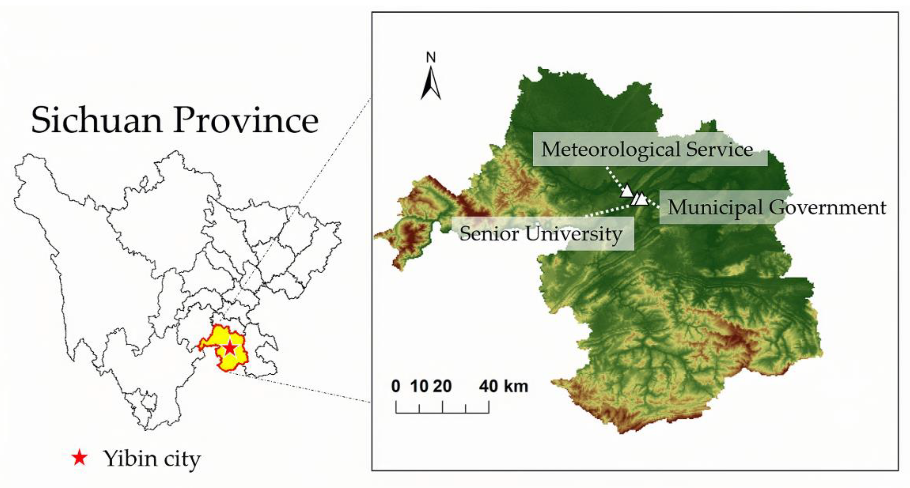
2.1. On-Line Sampling and Analysis

To better know the VOC characteristics in four seasons in Yibin, the VOC data we measured were from a long-term sampling site on the roof of a senior university. To facilitate the analysis, trace pollutant concentrations and meteorological data from the nearest state controlling monitoring stations were also obtained (Figure 1). The three different sites we mentioned collected different monitoring data. The VOCs were enriched through a low-temperature preconcentration unit (Models AC-GCMS1000, HEXIN MASS Spectrometry, Guangzhou, China) and analyzed by a gas chromatography-mass detector/flame ionization detector (GC–MS/FID, Models 7890A/59777B, Agilent, California, USA). Finally, 112 VOC species were quantitatively detected. Hourly measurements of trace pollutants (including O3, NO2, CO, SO2, CO2, PM2.5) were monitored and maintained through the national monitoring station of the Municipal Government, and related data were obtained from a publicly available data site website (http://www.scnewair.cn/, accessed on 15 March 2022). Meteorological data (including temperature, relative humidity, pressure, wind speed, and wind direction) were derived from the Yibin Meteorological Service (station number 56492, http://www.scnewair.cn/, accessed on 26 May 2022)

2.2. Methodology

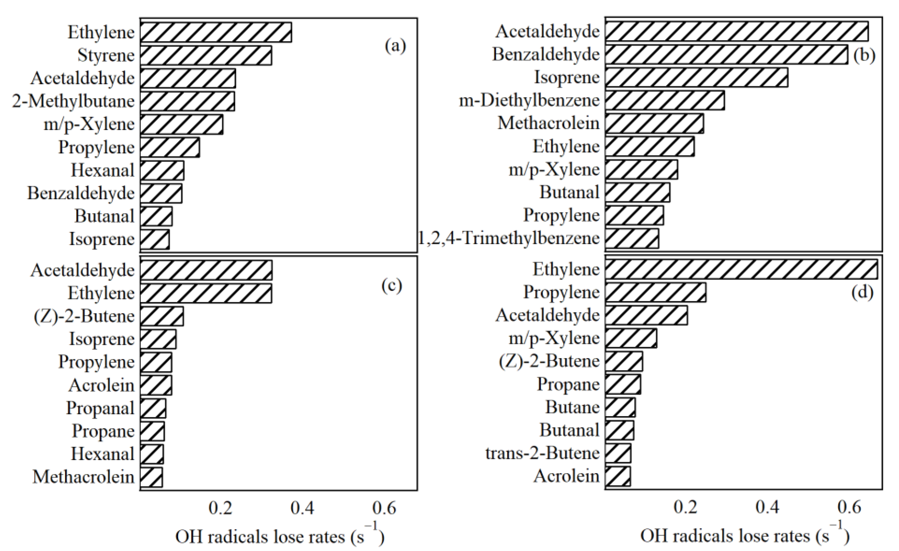
2.2.1. The OH Loss Rate of VOCs (LOH)

Because the reactions of VOCs with OH radicals are the starting points of photochemical oxidation for VOCs, the OH-responsive LOH becomes an important indicator of the VOC reactivates in a region, as shown in Equation (1):
L i OH = [ VOC ] i   ×   K i OH
where L i OH is the rate of OH radical consumption (s−1) by VOC component i, [ VOC ] i is the molecule number mixing ratio (molecule/cm3) of VOC species i, and K i OH   is the reaction rate constant of VOC component i with OH radicals in the atmosphere (cm3/molecule · s); the K i OH for 100 VOCs species were derived from Atkinson [31].

2.2.2. Ozone Formation Potential (OFP)

The maximum incremental reactivity (MIR) is commonly used to calculate the ozone formation potential (OFP) of each VOC species to indicate the maximum contribution of a single VOC species to ozone production, as shown in Equation (2):
OFP i   = [ VOC ] i   ×   MIR i
where OFP i   is the ozone formation potential (μg/m3) of VOC component i, [ VOC ] i is the mass mixing ratio (μg/m3) of VOC species i in the measured atmospheric environment, and MIR i is the maximum incremental reactivity of VOC component i; the MIR i for 53 VOCs were obtained from the research team of Shandong University, which was developed on the domestic environment to better calculate OFP values [32].

2.2.3. Secondary Organic Aerosol Formation Potential (SOAP)

VOCs are essential contributors for forming secondary pollutants of SOA, and the FAC coefficient is universally used to calculate SOAPs, as shown in Equation (3):
SOAP i = [ VOC ] i / ( 1     F VOCr i )   ×   FAC i
where   SOAP i   means the SOA formed of VOC component i, [ VOC ] i is the mixing ratio of VOC species i in an ambient atmosphere, F VOCr i is the fraction of reacted VOC species i, and   FAC i represents the fractional aerosol coefficients from each VOC species, which were accessed by Grosjean [33].

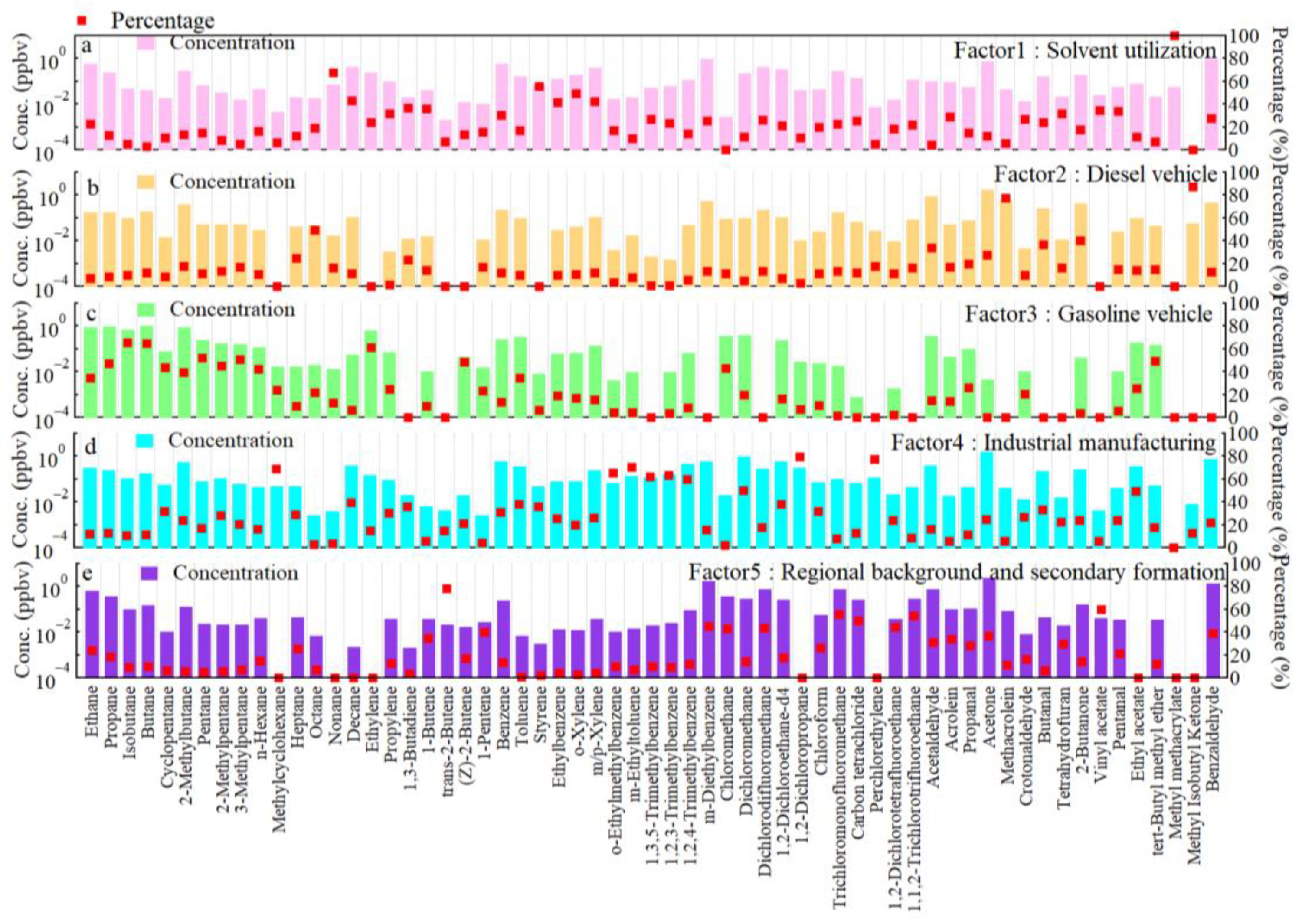
2.2.4. Positive Matrix Factorization (PMF)

The PMF model is a conventional way to drill down VOC source apportionment and has been universally used in some research [34,35,36]. This study used the US EPA PMF 5.0 (Washington, DC, USA) model to analyze the main VOC sources in the spring, summer, fall, and winter, to show seasonal variation.
Before running PMF, there are two input files need to be prepared, including a matrix of species concentrations and another matrix for concentration uncertainties. The uncertainty is determined by the relation between the concentration and MDL of VOC species; if the concentration is higher, the uncertainty values could be calculated by Equation (4), and otherwise by Equation (5):
Uncertainty = ( error   fraction   ×   concentration ) 2 + ( 0 . 5   ×   MDL ) 2
Uncertainty = 5 6   ×   MDL
where MDL represents the method detection limit, and the error fraction represents the relative measurement error (as 10% in this study).
After inputting the VOC data, the model can calculate the S/N (signal-to-noise ratio) values for each species, and there is a correction in the calculation of S/N values in PMF 5.0. In the corrected calculation, only the concentration values that exceed the uncertainty are included in the calculation, affecting the S (signal value) part of the S/N calculation. S/N < 1 is classified as “weak”, and S/N > 1 is classified as “strong”. In addition, the classification of species can also be set according to the data quality of a species in the actual observation, such as the time series of species’ concentration, the scatter plot of concentration and uncertainty, and the correlation between species.
In the data processing, the VOC data in April, July, October and January were applied to represent the overall level in spring, summer, fall. and winter, respectively.

3. Results and Discussions

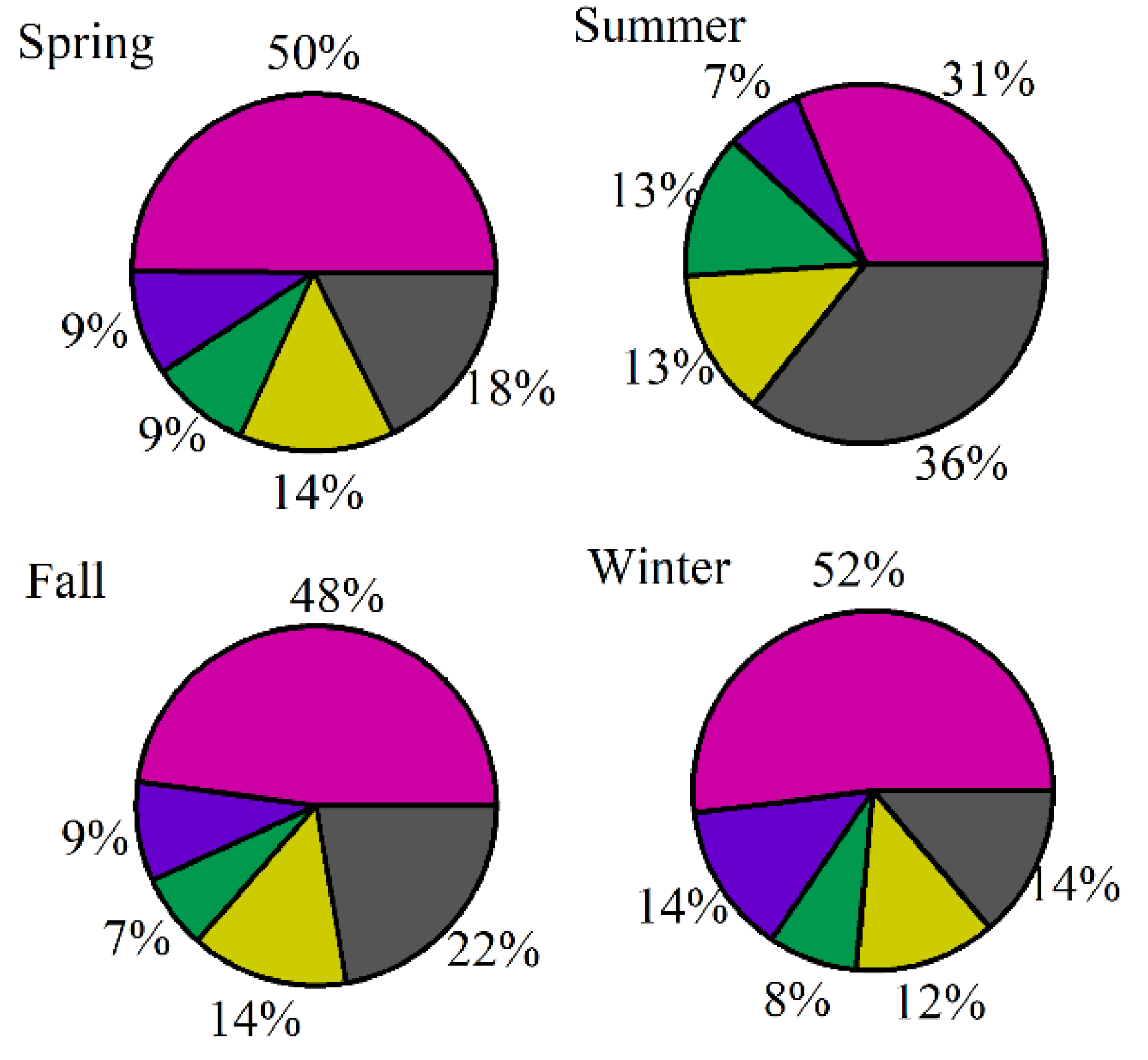
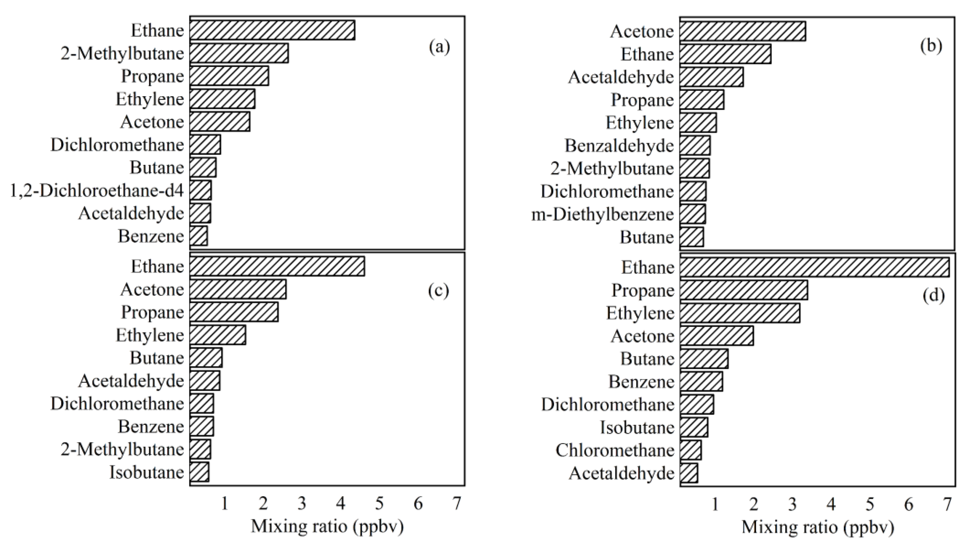
3.1. Basic Data Analysis

The factors that influence the urban air pollution situation were not only the emission sources and the pollution characteristics of the pollutants, but also the meteorological parameters. As provided in Figure S1, the variation in the daily average values of the main meteorological parameters during the observation period was given, and the average temperature in the four seasons was the lowest in winter 2022, 8.8 °C, varying between 7.7–10.9 °C, and the highest in summer 2021, 27.2 °C, varying between 23.7–30.8 °C. It could not be seen that the temperature and humidity showed a more obvious negative correlation with the variation of wind speed in Yibin’s urban area in each season. A total of 112 VOC species monitored by the online equipment (Table S1) were divided into five categories: alkanes, alkenes, aromatics, halohydrocarbons, and OVOCs.
Figure 2 shows the changes in mixing ratios and the percentage of components at the VOC component monitoring sites in April (spring), July (summer), October (fall), and January (winter). Figure 3 shows that alkanes account for more than 50%, and the largest share is in spring and winter, with average mixing ratios of 11.5 ppbv and 14.0 ppbv, respectively; OVOCs are the largest mixing ratio component in summer, with an average mixing ratio of 8.2 ppbv, and alkanes are second only to OVOCs, with an average mixing ratio of 7.2 ppbv. To further explore the dominant species of specific VOCs, as shown in Figure 4, the species in different seasons were basically the same, accounting for about 70% of the total VOCs; the dominant species of VOCs in Yibin urban area were mainly C2–C5 alkanes. Ethane was the most dominant species in winter, spring, and fall, with average mixing ratios up to 7.1 ppbv, 4.4 ppbv, and 4.6 ppbv, while acetone was the most dominant species in summer, with mixing ratios up to 3.4 ppbv. The greatest variation in mixing ratio among the seasons was observed for acetaldehyde and ethylene, with acetaldehyde in summer (1.8 ppbv) being 3.2 times higher than in winter, 2.1 times higher than in fall, and 1.8 times higher than in spring, and ethylene in winter (3.2 ppbv) being 3.0 times higher than in summer, 2.7 times higher than in spring, and 2.7 times higher than in fall. Among the main dominant species, acetaldehyde and acetone had higher mixing ratios in summer than in the rest of the seasons, and the rest of the dominant species were all higher in winter than in the rest of the seasons.

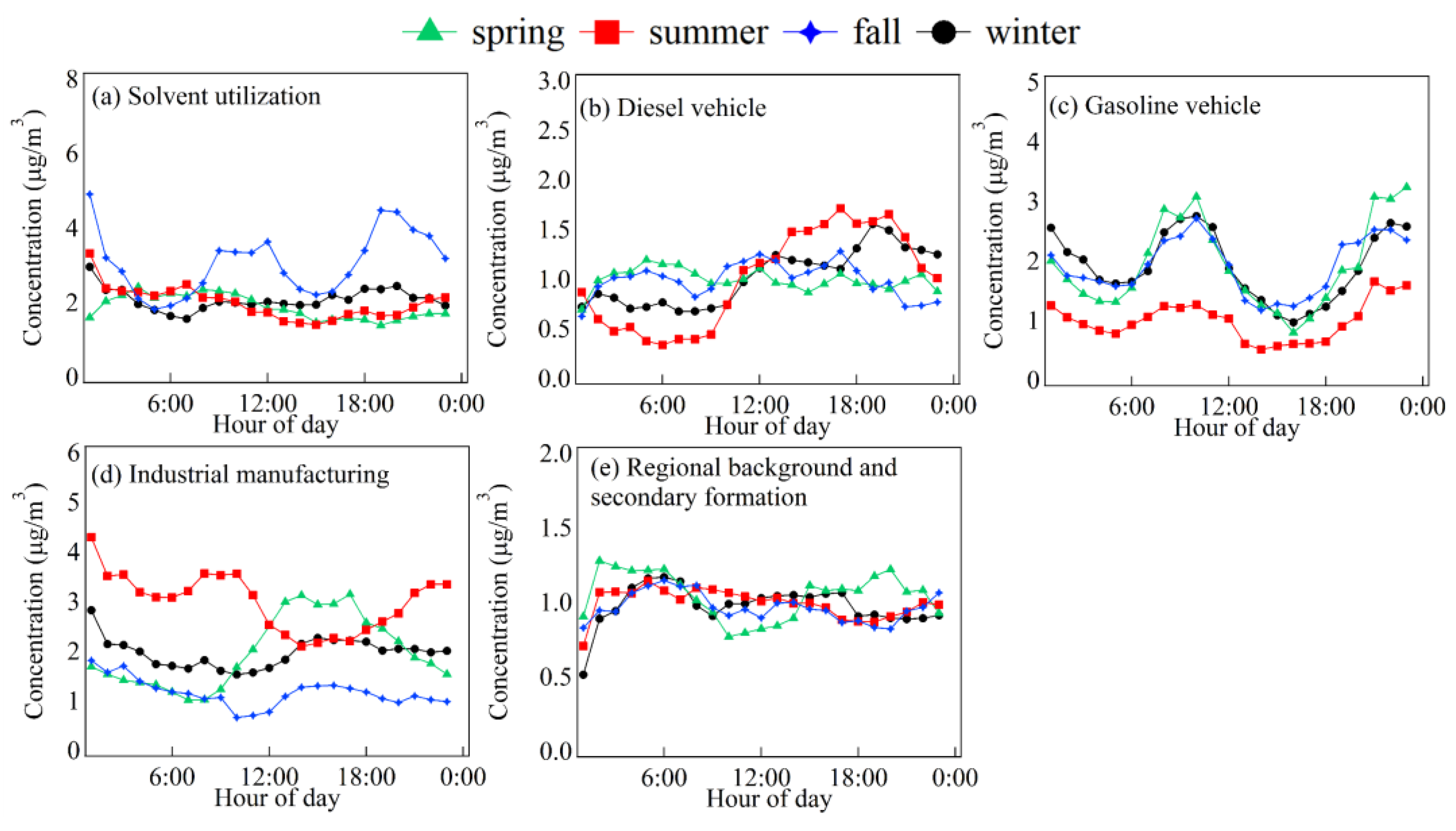
3.2. Diurnal Variation Characteristics

The daily variation characteristics of atmospheric pollutants were the result of a combination of meteorological, primary emission, and atmospheric chemical processes. The diurnal variability of typical VOCs near the observation site was illustrated in Figure 5. The diurnal variation of VOC species could be affected by abundant factors, and the features of diurnal changes could also display the transportation, sources, and chemical reaction of ambient VOCs [37]. Overall, evening peak values of TVOCs, except for halohydrocarbons, were higher than their morning peak values. This was maybe caused by the lower boundary layer height at night than daytime, which was adverse for the vertical and mixed spreading out of VOC pollutants [38,39,40].
It could be seen that the seasonal daily variation of alkanes species was basically consistent, with the peak in spring occurring 2–3 h later than the other seasons, and only one obvious peak was caused by the high emission of 3-methylpentane at 14:00, while the other seasons showed two peaks, with more prominent emissions at night (21:00–1:00) and early morning (8:00–12:00). The average hourly mixing ratio in winter was significantly higher than the other seasons.
The daily trend of alkenes species showed a good consistency with two peaks, which were more prominent in the morning (8:00) and evening (22:00–1:00). The lowest value was reached in the afternoon (16:00), and the average hourly mixing ratios in winter were much higher than those in other seasons.
The daily variation trend of aromatics species season showed a good consistency, and generally appears with multiple peaks, and the daily variation trend was more consistent with CO and NO2: the first peak occurs in the early morning (8:00–11:00), which was consistent with the morning rush hour, and was a typical traffic source emission characteristic, and the peak point of emission occurs in the evening (21:00–22:00). The highest point of variation appeared at 1:00 a.m. There may be nighttime industrial solvent processing at this site, which may also be caused by the reduced boundary layer mixing ratio at night.
The daily variation of halohydrocarbons species showed three peaks in the early morning (0:00–2:00), noontime (11:00–13:00), and afternoon (13:00–17:00), and the highest daily variation point occurred at 1:00 a.m., the same time as the highest value of aromatic hydrocarbons, presumably due to industrial emissions at night.
The daily variation in OVOC species was characterized by a single peak, which occurs after midday, similar to the trend in daily variation in the ozone. The peak of OVOCs occurs at the same time as the trough of CO, and the increasing trend of OVOCs in the morning was associated with not only the secondary oxidation reaction [41,42] but also primary anthropogenic emissions. Moreover, the mixing ratio of OVOCs decreased continuously from 1:00 a.m. to 6:00 a.m., and showed a larger decrease at 7:00. The mixing ratios of OVOCs continued to decrease from 1:00 a.m. to 6:00 a.m., and then increased significantly from 7:00 a.m. to 16:00 a.m. to 18:00 a.m. After reaching their peak point, they maintained a stable change. The mixing ratio levels of OVOCs remained high at night, which may be due to the accumulation of NMHCs or the weakening of the photochemical reaction of OVOCs themselves. In addition, the decrease in the height of the mixed boundary layer during this time may also cause the pollutant mixing ratios to increase.

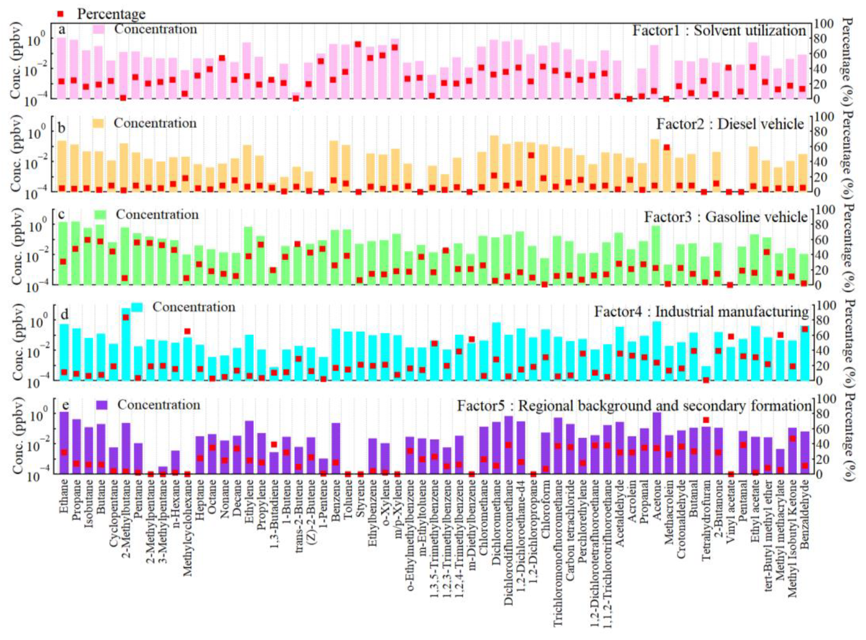
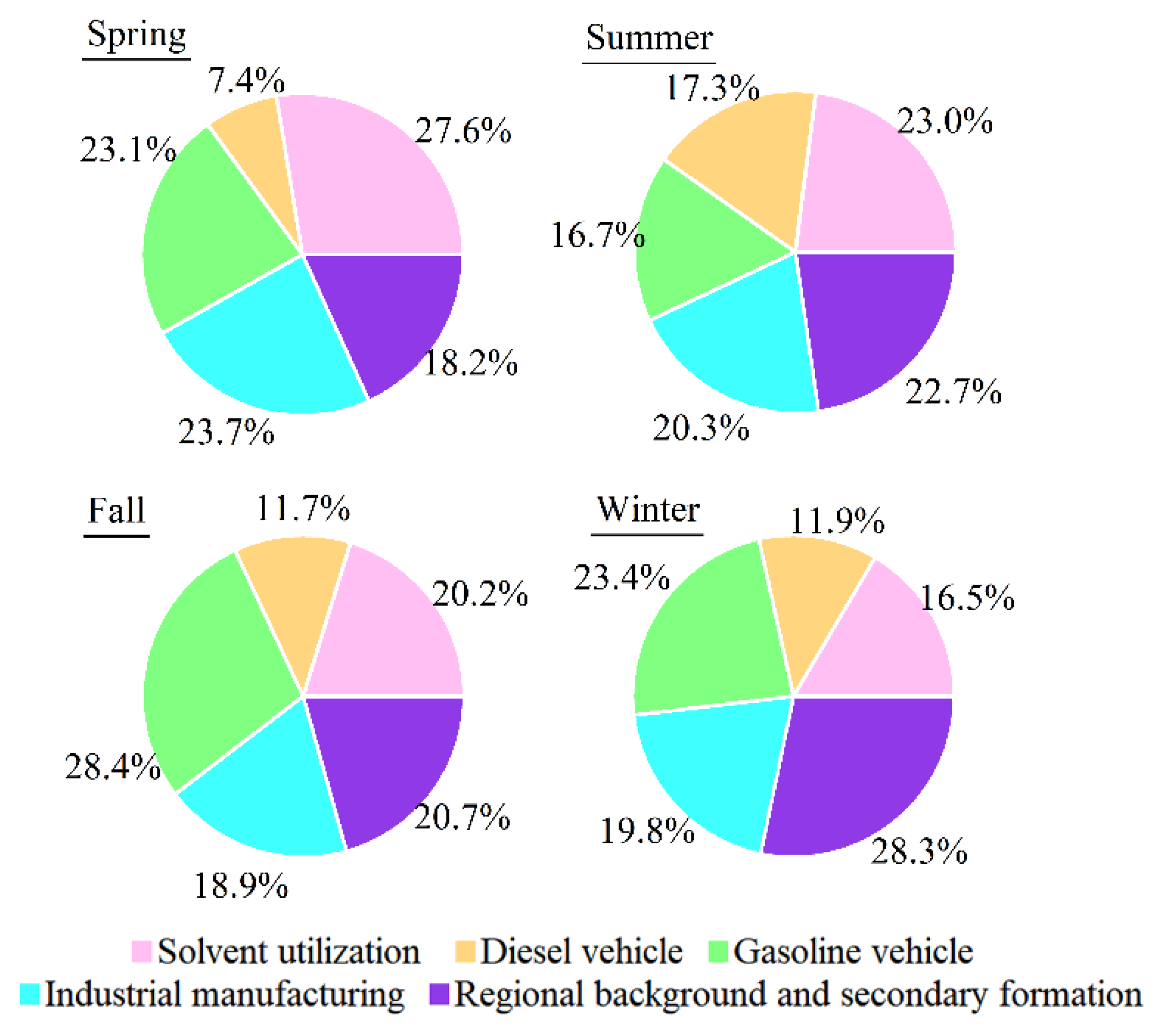
3.3. Source Apportionment of VOCs in Yibin

To better know the potential reason for regional pollution and to implement control strategies, it was appropriate to judge regional VOCs source contributions [43]. For the data analysis of VOCs in four seasons, 61 characteristic VOCs species were selected and input into the PMF model, and five types of source factors were resolved by error analysis and ordered the same in four seasons; the specific mixing ratio and percentage of PMF results in different seasons are provided in Table S2, and the concise graphs are shown in Figure 6, Figure 7, Figure 8 and Figure 9.
Source 1 (Figure 6a, Figure 7a, Figure 8a and Figure 9a) was assigned to solvent utilization, which contained high loadings of aromatics (ethylbenzene, toluene, o-xylene, m/p-xylene), ethyl acetate, and a certain level of long-chain alkanes. Ethyl acetate was a typical component of VOCs emitted from furniture spraying/oil-based paint [44], and toluene was usually used as an organic solvent species [45], so factor 1 was judged to be solvent utilization sources.
Source 2 (Figure 6b, Figure 7b, Figure 8b and Figure 9b) was assigned to diesel vehicles, which had a high content of high-C number alkanes (octane and nonane) and aromatics (benzene and toluene). These compounds are typical emissions of diesel vehicles [46], so factor 2 was judged as diesel vehicle sources.
Source 3 (Figure 6c, Figure 7c, Figure 8c and Figure 9c) was characterized by high contents of low-carbon alkanes (ethane, propane, isobutane, n-butane, and pentane), (z)-2-butene, and tert-butyl methyl ether, indicating that it was related to gasoline vehicle emissions. Ethylene and propylene were produced by internal combustion engines, and tert-butyl methyl ether was used as an addictive to improve the anti-knock performance of gasoline [47]. The results suggest that factor 3 was gasoline vehicle sources.
Source 4 (Figure 6d, Figure 7d, Figure 8d and Figure 9d) was considered to be industrial manufacturing, which has a high content of methylcyclohexane, dichloromethane, 1,2-dichloropropane, methacrolein, 2-butanone, and ethyl acetate. Dichloromethane was high in the emissions of chlorination plants [48], and 1,2-dichloropropane could be emitted from some industrial plants [49], so factor 4 was judged as industrial manufacturing.
Source 5 (Figure 6e, Figure 7e, Figure 8e and Figure 9e) was assigned to be regional background and secondary formation sources, which was characterized by high level of methylcyclohexane, dichlorodifluoromethane, trichloromonofluoromethane, 1,2-dichlorotetrafluoroethane, and 1,1,2-trichlorotrifluoroethane. It showed low amounts of hydrocarbons but relatively higher OVOCs (acetone, vinyl acetate, and pentanal), implying that factor 5 could be secondary formations in the air [50]. The fluorine-containing halogenated hydrocarbons mainly originated from the manufacture of refrigerants with strong chemical lifetimes and low chemical reactivity, so factor 5 was judged to be a regional background and secondary formation source.
Figure 10 showed the proportion of five sources in all seasons, and it was obvious that vehicle sources including gasoline and diesel vehicles together contributed the most of VOCs, which followed the sequence of fall (40.1%) > winter (35.3%) > summer (34.0%) > spring (30.5%). Moreover, gasoline vehicle sources contributed more than diesel vehicles in spring (23.1%, 7.4%), fall (28.4%, 11.7%), and winter (23.4%, 11.9%), but conversely in summer (16.7%, 17.3%). Solvent utilization cannot be ignored for its significant contribution to VOCs of spring (27.6%) > summer (23.0%) > fall (20.2%) > winter (16.5%). The percentages of industrial manufacturing sources in four seasons were nearly the same level for spring (23.7%) > summer > (20.3%) > winter (19.8%) > fall (18.9%). Regional background and secondary formation sources contributed similarly in summer (22.7%) > fall (20.7%) > spring (18.2%).
As shown in Figure 11, the diurnal variation in solvent utilization has a decrease in VOC concentrations in the early morning, which was likely due to enhanced photochemical loss and decreased emissions, and then the concentration of solvent emissions increased from 15:00 to 17:00. For diesel vehicle emissions, the source contribution has a sudden increase from 8:00 until 18:00, which was consistent with the human work schedule, with high loadings during the daytime and low loadings at nighttime. Gasoline vehicles showed two distinct peaks during the morning and evening, which were in line with rush hour traffic. It can be seen that the first peak appeared at about 9:00 and the second appeared at around 21:00 in four seasons due to a reduced mixing height and strengthened traffic emissions. Industrial manufacturing indicated that other seasons besides summer were characterized by high VOC concentrations during the afternoon due to high emissions and low concentrations during nighttime. Regional background and secondary formation emissions exhibited a maintenance of the VOC concentration level until midnight.

3.4. VOC Reactivities and Potentials to Secondary Pollutants

3.4.1. LOH of VOC Species

The total OH loss rates (LOH) of the measured VOC species in this work were 2.9 s−1, 4.4 s−1, 2.0 s−1, and 2.5 s−1 in spring, summer, fall, and winter, respectively (Table S3). Alkenes were the main reactive VOC group (Table S2). The alkenes accounted for 4.7%, 3.6%, 5.6%, 7.4% of TVOCs in spring, summer, fall, and winter, respectively, but they had the highest contribution to LOH, and their contributions to LOH were 27.7%, 22.6%, 36.8%, 47.3% in the four seasons, respectively. The higher mixing ratio of alkanes had a relatively small contribution to LOH, while halohydrocarbons had the lowest contribution to LOH.
Among the top ten species contributing to LOH (Figure 12a–d), ethylene contributed the most to LOH in spring, fall, and winter, because of the high-rate constant, while in summer, acetaldehyde ranked first.

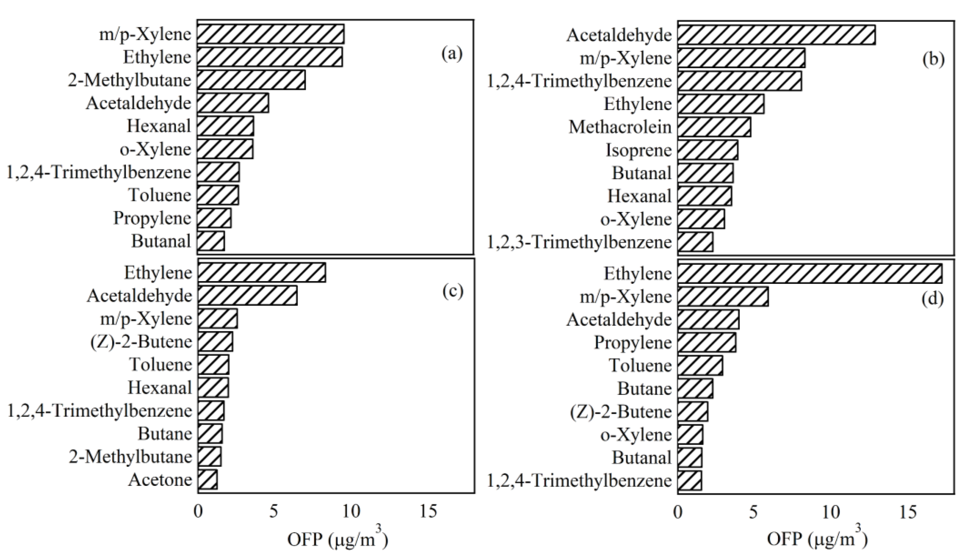
3.4.2. OFP of Ambient VOCs
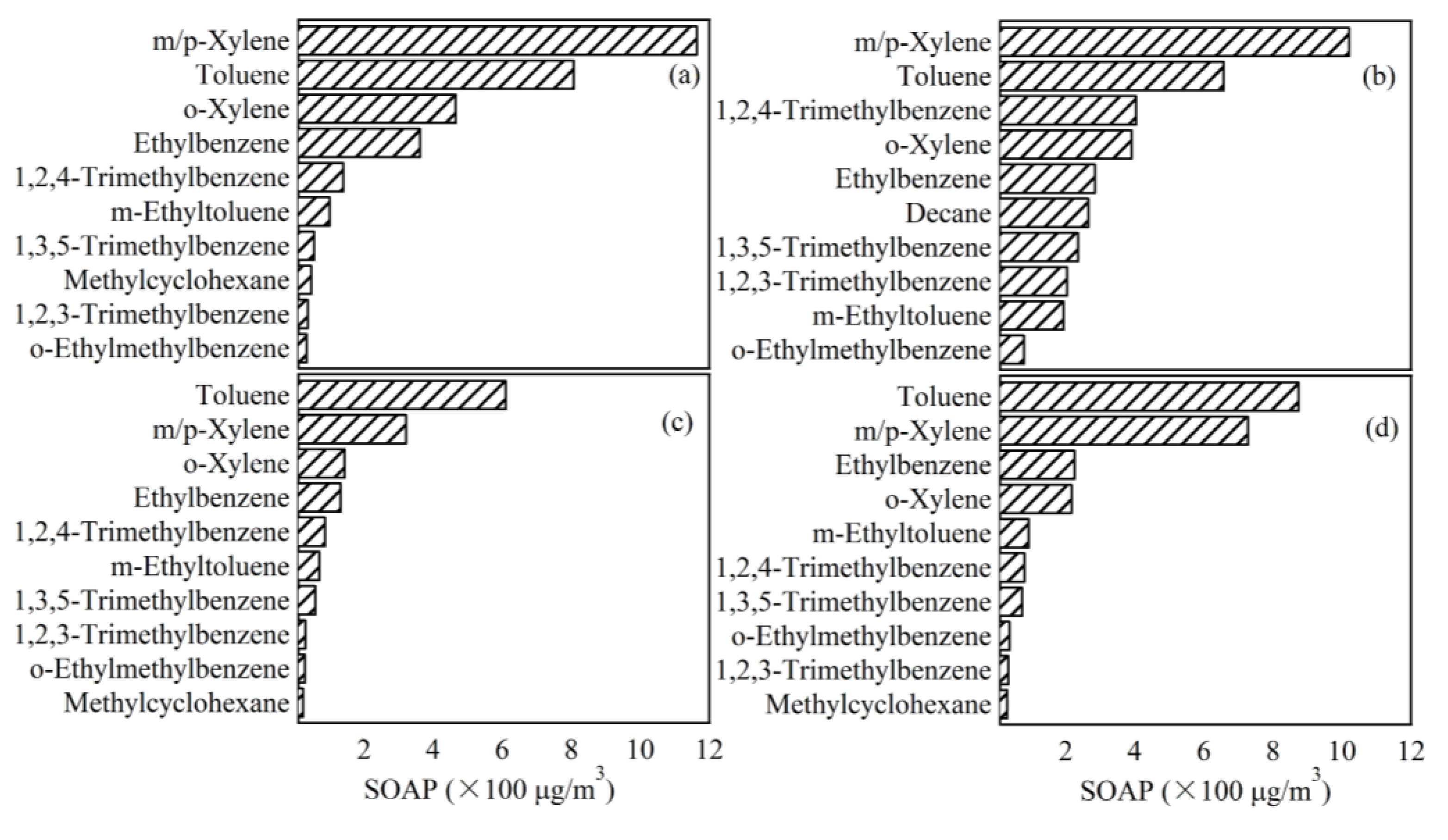
To estimate the contribution to the formation of O3 at the ground level, the OFP method was applied in this work. The OFP values calculated included 53 VOC species (Table S4). As shown in Figure 13, alkenes and OVOCs were the major contributors to OFP in all seasons. Although, alkenes and OVOCs had a lower proportion of the TVOC mixing ratio, they were considered to play significant roles in O3 formation [51].
The top ten VOC species contributing to total OFPs were given in Figure 14a–d. These species contributed the majority of the total OFPs, with contributions of 66.7%, 68.4%, 63.0%, and 69.6% in spring, summer, fall, and winter, respectively. Controlling these target VOC emissions would likely have a positive impact on O3 abatement [19]. Among the top ten OFP contributors, ethylene and acetaldehyde showed higher photochemical reaction reactivity and contributed most of the OFP. Isoprene, as a marker of biogenic VOCs, showed certain high OFPs in summer, which indicated that biogenic emissions might have significant roles in the formation of ground-level O3 in Yibin.

3.4.3. SOAP of VOCs

The calculated SOAP values were 0.25 μg/m3, 0.34 μg/m3, 0.39 μg/m3, and 0.16 μg/m3 in spring, summer, fall, and winter, respectively (Table S5). The most important contributors to SOA were aromatics. The top ten VOC species contributing to the total SOAP are listed in Figure 15a–d. The VOC species with the largest contribution to SOA in all seasons were toluene, m/p-xylene, and o-xylene. Generally, the formation of SOA was considered to be characterized mainly by aromatics [52,53]. Therefore, proper controlling of these compounds would have positive impacts on secondary pollution control.

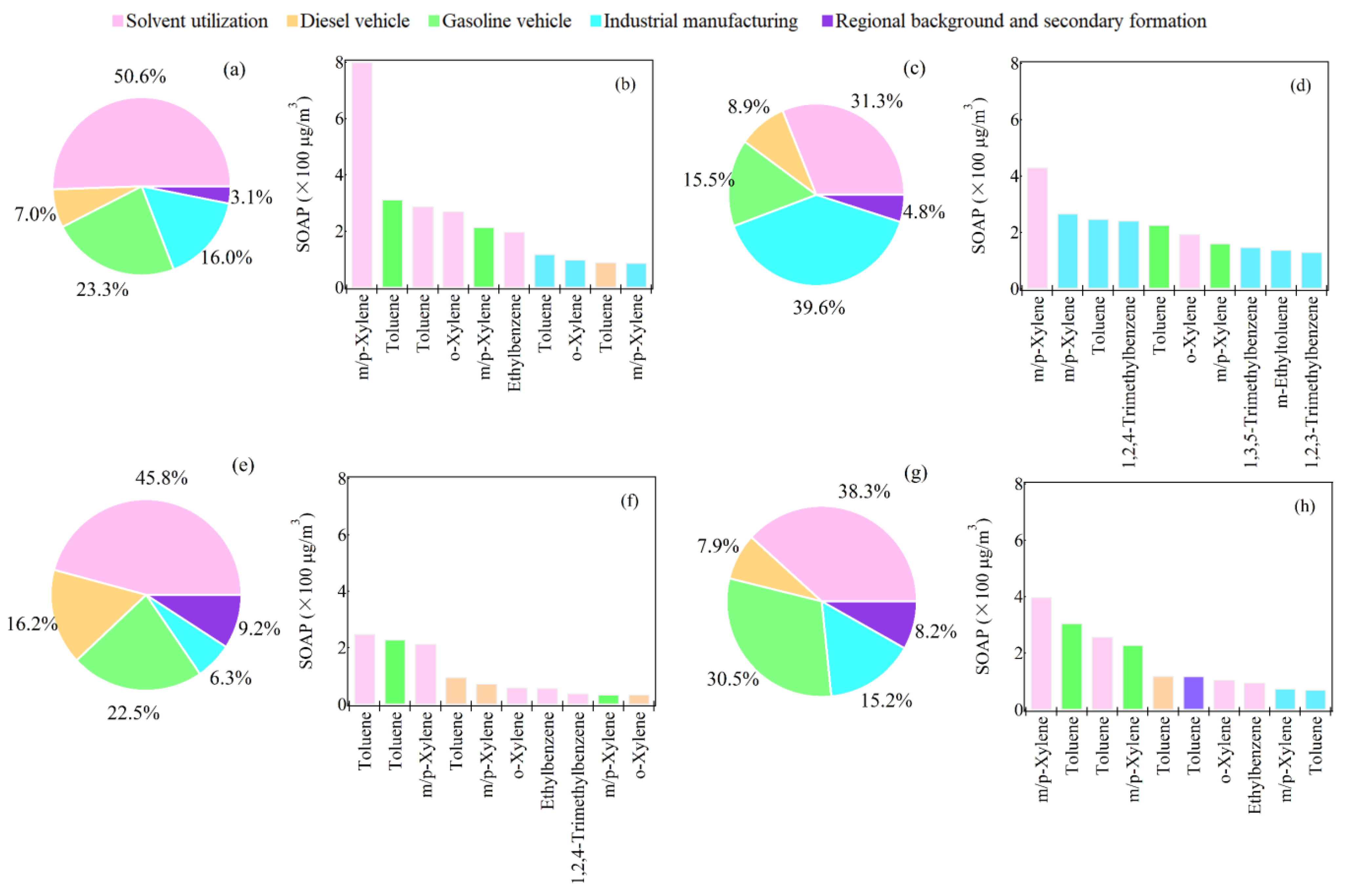
3.5. Contributions of VOC Sources to the Secondary Pollutant Formation

In Section 3.4.2 and Section 3.4.3, we have discussed the O3 formation potential of applying the MIR method to assess the reactivates of the VOC species, and discussed the SOA formation potential of applying the FAC method to assess the reactivates of the VOC species. Here, we tried to evaluate the O3 and SOA formation potential for each source depending on the concentration profile of each VOC species in the corresponding source derived from PMF model [54]. Therefore, we used the same method to calculate the contributions of VOC sources to O3 and SOA formation. Figure 16a,c,e,g, presented the contributions of different VOC sources extracted from PMF to the OFP values in different seasons, respectively. In spring, solvent utilization had the largest OFPs (36.8 μg/m3), accounting for 30.4% of the total OFP values. This was due to the high loadings of relative aromatics in this source profile, followed by gasoline vehicles (32.2 μg/m3, 26.6%), industrial manufacturing (30.6 μg/m3, 25.2%), regional background and secondary formation (14.0 μg/m3, 11.5%), and diesel vehicles (7.7 μg/m3, 6.4%).
In summer, the OFP value of industrial manufacturing became the highest (39.4 μg/m3), and the proportion increased to twice that value in summer (27.7%). The order of contribution of the other sources to OFP was greatly changed, followed by solvent utilization (28.9 μg/m3, 20.3%), diesel vehicles (27.8 μg/m3, 19.5%), gasoline vehicles (26.5 μg/m3, 18.6%), and regional background and secondary formation (29.6 μg/m3, 13.8%). In all, the contributions of OFPs from the regional background was stable.
In fall, the contribution of solvent utilization sources to OFPs during the fall was 34.7%, making solvent utilization the largest source of emissions, followed by gasoline vehicles (23.3 μg/m3, 28.3%), industrial manufacturing (13.0 μg/m3, 15.8%), regional background and secondary formation (11.5 μg/m3, 14%), and diesel vehicles (5.9 μg/m3, 7.2%).
In the winter, gasoline vehicles had the largest proportion of OFPs (48.2 μg/m3, 39.5%), followed by solvent utilization (21.3 μg/m3, 17.5%), diesel vehicles (20.3 μg/m3, 16.7%), industrial manufacturing (16.1 μg/m3, 13.2%), and regional background and secondary formation (16.0 μg/m3, 13.1%). All in all, gasoline vehicles contributed the most of OFPs; therefore, proper controlling of gasoline vehicle emissions matters to the management of VOCs to reduce the formation of O3 and photochemical pollution in Yibin city.
Figure 16b,d,f,h showed the top ten OFP contributors of VOCs from different sources. We found that m/p-xylene, ethylene from the emissions of solvent utilization, 2-methylbutane and 1,2,4-trimethylbenzene from industrial manufacturing, acetaldehyde, and ethylene from diesel vehicles were the main species of VOC emissions contributing to the formation of the photochemical O3. Therefore, the emissions of specific VOC species should not be ignored, though there was a small amount of VOC species that could be monitored to effectively alleviate photochemical pollution in Yibin. Solvent utilization contributed most in the spring, fall, and winter, which indicated that during these periods, there was a need to focus more on the mixing ratio of aromatics, as the source of aromatics was mainly from solvent utilization.
Figure 17a,c,e,g present the contributions of different VOC sources extracted from PMF to the SOAP values in different seasons, respectively.
Generally, the results showed that the proportion and SOAP value of solvent utilization sources followed the sequence of spring (0.3 μg/m3, 50.6%) > fall (0.2 μg/m3, 45.8%) > winter (0.2 μg/m3, 38.3%) > summer (0.1 μg/m3, 31.3%). During spring and fall, solvent utilization made the dominant contribution to SOAPs, which may be affected by the temperature of these two seasons. When it came to diesel vehicle sources, the proportion sequence changed into fall (16.2%) > summer (8.9%) > winter (7.9%) > spring (7.0%), while the SOAP value of diesel vehicles was similar during fall (0.07 μg/m3), summer (0.05 μg/m3), winter (0.05 μg/m3), all better than spring (0.04 μg/m3). Gasoline vehicles had the order of spring (30.5%) > winter (23.3%) > summer (22.5%) > fall (15.5%). The proportion sequence from industrial manufacturing was summer (39.6%) > spring (16.0%) > winter (15.2%) > fall (6.3%), while the SOAP value in summer (0.30 μg/m3) was the largest. The proportion order of regional background and secondary formation was fall (9.2%) > winter (8.2%) > summer (4.8%) > spring (3.1%), while the SOAP value in winter (0.04 μg/m3) and summer (0.04 µg/m3) were larger than other two seasons. More focus should be put on industrial manufacturing emissions in summer for their high contribution to SOAPs. Figure 17b,d,f,h showed the top ten SOAP contributors of VOCs from different sources. We found that m/p-xylene from the emissions of solvent utilization and toluene from gasoline vehicle were the main species of VOC emissions contributing to the formation of SOA. Therefore, in order to reduce SOA formation in Yibin, emissions of VOCs in gasoline vehicles and solvent utilization should be reduced as far as possible. When analyzing the local secondary pollution situation in Yibin city, it was not only necessary to consider the mixing ratio of VOCs, but also to focus on identifying the sources that have the greatest impact on local emissions, and then to analyze the specific VOC species from the sources to achieve the precise and effective control of local secondary pollution status.

4. Conclusions

In this research, the measured VOC mixing ratios in Yibin were analyzed. The results suggested that the ambient VOC mixing ratios were characterized by alkanes (50%, 31%, 48%, 52%) and OVOCs (18%, 36%, 22%, 14%) in four seasons, followed by halohydrocarbons (14%, 14%), alkenes (10%, 9%), and aromatics (9%, 7%) in spring and fall, aromatics (13%), halohydrocarbons (13%), and alkenes (7%) in summer, and alkenes (14%), halohydrocarbons (13%), and aromatics (8%) in winter. Different season indicated different VOC characteristics. The comparison showed that the OVOCs were more dominant in summer than other seasons, which may be affected by the higher temperature in summer.
Additionally, five sources were received from the PMF model. The results showed that vehicle sources including gasoline and diesel vehicles together contributed the most VOCs in all seasons, and the percentages of each season fluctuated between 30.5% and 40.1%. Solvent utilization was also important in emissions, which had the ratio of 16.5–27.6% in four seasons, the proportion of industrial manufacturing changed between 18.9–23.7%, and regional background and secondary formation accounted for 18.2–28.3% in different seasons.
Through the calculation of OFPs and SOAPs, we could initially find that m/p-xylene, toluene, and ethylene contribute a larger proportion of all the species mentioned above. As for the source contributions to OFPs and SOAPs, we found that contributions to secondary pollutants by different sources varied across seasons. In spring, solvent utilization (OFP 30.4%; SOAP 50.6%) was the dominant source, followed by gasoline vehicles (OFP 26.6%; SOAP 23.3%) and industrial manufacturing (OFP 25.2%; SOAP 16.0%); in summer, the major source was gasoline vehicles (OFP 26.6%; SOAP 15.5%) and solvent utilization (OFP 20.3%; SOAP 31.3%); in fall, solvent utilization (OFP 34.7%; SOAP 45.8%) made the greatest contribution to secondary formation, followed by gasoline vehicles (OFP 28.3%; SOAP 22.5%); in winter, gasoline vehicles (OFP 39.5%; SOAP 30.5%) and solvent utilization (OFP 17.5%; SOAP 38.3%) were the dominant sources. In order to reduce the ambient VOCs to comply with the atmospheric standards, priority should be given to gasoline vehicle and solvent utilization emissions. Overall, all the studies are of benefit for the precise emission control of VOCs in the Yibin region, and are further useful for VOC emission control strategy in other cities.

Supplementary Materials

The following supporting information can be downloaded at: https://www.mdpi.com/article/10.3390/atmos13091389/s1, Figure S1: Time series of Temperature and RH; Table S1: The measured VOCs species; Table S2: Source profiles calculated by PMF model; Table S3: The contributions of VOCs to LOH in spring, summer, fall, winter; Table S4: The contributions of VOCs to OFP in spring, summer, fall, winter; Table S5: The contributions of VOCs to SOAP in spring, summer, fall, winter.

Author Contributions

Investigation, L.K., T.L.; Methodology, X.J., S.Z., L.K. and D.C.; data curation, L.K., T.L.; writing—original draft preparation, L.K.; writing—review and editing, G.H., F.Y.; discussion of the results, Y.L., F.Y. All authors have read and agreed to the published version of the manuscript.

Funding

This research was supported by the Yibin Ecological Environment Bureau and Chengdu Science and Technology Bureau, grant number No. 2020-YF09-00051-SN.

Institutional Review Board Statement

No applicable.

Informed Consent Statement

No applicable.

Data Availability Statement

Data are available upon request on the official website of the Yibin Ecological and Environmental Monitoring Center.

Conflicts of Interest

The authors declare no conflict of interest.

References

  1. Forstner, H.J.L.; Flagan, R.C.; Seinfeld, J.H. Secondary organic aerosol from the photooxidation of aromatic hydrocarbons: Molecular composition. Environ. Sci. Technol. 1997, 31, 1345–1358. [Google Scholar] [CrossRef]
  2. O’Dowd, C.D.; Aalto, P.; Hameri, K.; Kulmala, M.; Hoffmann, T. Aerosol formation—Atmospheric particles from organic vapours. Nature 2002, 416, 497–498. [Google Scholar] [CrossRef] [PubMed]
  3. Odum, J.R.; Jungkamp, T.P.W.; Griffifin, R.J.; Flagan, R.C.; Seinfeld, J.H. The atmospheric aerosol-forming potential of whole gasoline vapor. Science 1997, 276, 96–99. [Google Scholar] [CrossRef] [PubMed]
  4. Atkinson, R. Atmospheric chemistry of VOCs and NOx. Atmos. Environ. 2000, 34, 2063–2101. [Google Scholar] [CrossRef]
  5. Sato, K.; Takami, A.; Isozaki, T.; Hikida, T.; Shimono, A.; Imamura, T. Mass spectrometric study of secondary organic aerosol formed from the photo-oxidation of aromatic hydrocarbons. Atmos. Environ. 2010, 44, 1080–1087. [Google Scholar] [CrossRef]
  6. Atkinson, R. Gas-phase tropospheric chemistry of organic compounds. J. Phys. Chem. 1994, 2, 11–216. [Google Scholar]
  7. Atkinson, R.; Tuazon, E.C.; Carter, W.P.L. Extent of H-atom abstraction from the reaction of the OH radical with 1-butene under atmospheric conditions. J. Chem. Kinet. 1995, 17, 725–734. [Google Scholar] [CrossRef]
  8. Lee, S.C.; Chiu, M.Y.; Ho, K.F.; Zou, S.C.; Wang, X. Volatile organic compounds (VOCs) in urban atmosphere of Hong Kong. Chemosphere 2002, 48, 375–382. [Google Scholar] [CrossRef]
  9. Dechapanya, W.; Eusebi, A.; Kimura, Y.; Allen, D.T. Secondary oganic aerosol formation from aromatic precursors. 1. Mechanisms for individual hydrocarbons. Environ. Sci. Technol. 2003, 37, 3662–3670. [Google Scholar] [CrossRef]
  10. Nadal, M.; Mari, M.; Schuhmacher, M.; Domingo, J.L. Multi-compartmental environmental surveillance of a petrochemical area: Levels of micropollutants. Environ. Int. 2009, 35, 227–235. [Google Scholar] [CrossRef]
  11. Sopian, N.A.; Jalaludin, J.; Tamrin, S.B.M. Risk of respiratory health impairment among susceptible population living near petrochemical industry—A review article. Iran. J. Public Health 2016, 45, 8. [Google Scholar]
  12. Hsu, C.Y.; Chiang, H.C.; Shie, R.H.; Ku, C.H.; Lin, T.Y.; Chen, M.J.; Chen, N.T.; Chen, Y.C. Ambient VOCs in residential areas near a large-scale petrochemical complex: Spatiotemporal variation, source apportionment and health risk. Environ. Pollut. 2018, 240, 95–104. [Google Scholar] [CrossRef] [PubMed]
  13. Kampa, M.; Castanas, E. Human health effects of air pollution. Environ. Pollut. 2008, 151, 362–367. [Google Scholar] [CrossRef] [PubMed]
  14. De Smedt, I.; Stavrakou, T.; Müller, J.F.; van der A, R.J.; Van Roozendael, M. Trend detection in satellite observations of formaldehyde tropospheric columns. Geophys. Res. Lett. 2010, 37, L18808. [Google Scholar] [CrossRef]
  15. Lu, Z.; Zhang, Q.; Streets, D.G. Sulfur dioxide and primary carbonaceous aerosol emissions in China and India, 1996–2010. Atmos. Chem. Phys. 2011, 11, 9839–9864. [Google Scholar] [CrossRef]
  16. Feng, T.; Bei, N.; Huang, R.J.; Cao, J.; Zhang, Q.; Zhou, W.; Tie, X.; Liu, S.; Zhang, T.; Su, X.; et al. Summertime ozone formation in Xi’an and surrounding areas, China. Atmos. Chem. Phys. 2016, 16, 4323–4342. [Google Scholar] [CrossRef]
  17. Liu, Z.; Li, N.; Wang, N. Characterization and source identification of ambient VOCs in Jinan, China. Air Qual. Atmos Health 2016, 9, 285–291. [Google Scholar] [CrossRef]
  18. Zhu, H.L.; Gao, T.Y.; Zhang, J.B. Wintertime characteristic of peroxyacetyl nitrate in the Chengyu district of southwestern China. Environ. Sci. Pollut. Control Ser. 2018, 25, 23143–23156. [Google Scholar] [CrossRef]
  19. Sun, J.; Shen, Z.X.; Zhang, Y.; Zhang, Z.; Zhang, Q.; Zhang, T.; Niu, X.Y.; Huang, Y.; Cui, L.; Xu, H.M.; et al. Urban VOC profiles, possible sources, and its role in ozone formation for a summer campaign over Xi’an, China. Environ. Sci. Pollut. Control Ser. 2019, 26, 27769–27782. [Google Scholar] [CrossRef]
  20. Tan, Q.; Zhou, L.; Liu, H.; Feng, M.; Qiu, Y.; Yang, F.; Jiang, W.; Wei, F. Observation-Based Summer O3 Control Effect Evaluation: A Case Study in Chengdu, a Megacity in Sichuan Basin, China. Atmosphere 2020, 11, 1278. [Google Scholar] [CrossRef]
  21. Wei, W.; Cheng, S.; Li, G.; Wang, G.; Wang, H. Characteristics of volatile organic compounds (VOCs) emitted from a petroleum refinery in Beijing, China. Atmos. Environ. 2014, 89, 358–366. [Google Scholar] [CrossRef]
  22. Niu, Z.; Zhang, H.; Xu, Y.; Liao, X.; Xu, L.; Chen, J. Pollution characteristics of volatile organic compounds in the atmosphere of Haicang District in Xiamen City, Southeast China. J. Environ. Monit. 2012, 14, 1144–1151. [Google Scholar] [CrossRef] [PubMed]
  23. Liu, Y.; Shao, M.; Lu, S.; Chang, C.-C.; Wang, J.-L.; Chen, G. Volatile organic compound (VOC) measurements in the pearl river delta (PRD) region, China. Atmos. Chem. Phys. 2008, 8, 1531–1545. [Google Scholar] [CrossRef]
  24. Lu, S.H.; Bai, Y.H.; Chen, Y.K.; Zhao, J.; Wang, Z.H. The characteristics of volatile organic compounds (VOCs) emitted from motor vehicle in Beijing. China Environ. Sci. 2003, 23, 127–130. [Google Scholar]
  25. Chameides, W.L.; Fehsenfeld, F.; Rodgers, M.O.; Cardelino, C.; Martines, J.; Parrish, D.; Lonneman, W.; Lawson, D.R.; Rasmussen, R.A.; Zimmerman, P.; et al. Ozone precursor relationships in the ambient atmosphere. J. Geophys. Res. 1992, 97, 6037–6055. [Google Scholar] [CrossRef]
  26. Ran, L.; Zhao, C.S.; Geng, F.H.; Tie, X.; Tang, X.; Peng, L.; Zhou, G.Q.; Yu, Q.; Xu, J.M.; Guenther, A. Ozone photochemical production in urban Shanghai, China: Analysis based on ground level observations. J. Geophys. Res. 2009, 114, D15301. [Google Scholar] [CrossRef]
  27. Tie, X.; Madronich, S.; Li, G.H.; Ying, Z.M.; Weinheimer, A.; Apel, E.; Campos, T. Simulation of Mexico City plumes during the MIRAGE-Mex Field campaign using the WRF-Chem model. Atmos. Chem. Phys. 2009, 9, 4621–4638. [Google Scholar] [CrossRef]
  28. Geng, F.H.; Cai, C.; Tie, X.; Yu, Q.; An, J.; Peng, L.; Zhou, G.; Xu, J. Analysis of VOC emissions using PCA/APCS receptor model at city of Shanghai, China. J. Atmos. Chem. 2010, 62, 229–247. [Google Scholar] [CrossRef]
  29. Scheff, P.A.; Wadden, R.A. Receptor modeling of volatile organic compounds. 1. Emission inventory and validation. Environ. Sci. Technol. 1993, 27, 617–625. [Google Scholar] [CrossRef]
  30. Shu, Z.; Liu, Y.; Zhao, T.; Xia, J.; Li, Y. Elevated 3D structures of PM2.5 and impact of complex terrain-forcing circulations on heavy haze pollution over Sichuan Basin, China. Atmos. Chem. Phys. 2021, 21, 9253–9268. [Google Scholar] [CrossRef]
  31. Atkinson, R.; Arey, J. Atmospheric degradation of volatile organic compounds. Chem. Rev. 2003, 103, 4605–4638. [Google Scholar] [CrossRef] [PubMed]
  32. Zhang, Y.; Xue, L.; Carter, W.P.L.; Pei, C.; Chen, T.; Mu, J.; Wang, Y.; Zhang, Q.; Wang, W. Development of ozone reactivity scales for volatile organic compounds in a Chinese megacity. Atmos. Chem. Phys. 2021, 21, 11053–11068. [Google Scholar] [CrossRef]
  33. Grosjean, D. Insitu organic aerosol formation during a smog episode: Estimated production and chemical functionality. Atmos. Environ. 1992, 26, 953–963. [Google Scholar] [CrossRef]
  34. An, J.; Wang, J.; Zhang, Y.; Zhu, B. Source apportionment of volatile organic compounds in an urban environment at the Yangtze River Delta, China. Arch. Environ. Contam. 2017, 72, 335–348. [Google Scholar] [CrossRef]
  35. Zheng, H.; Kong, S.; Xing, X.; Mao, Y.; Hu, T.; Ding, Y.; Li, G.; Liu, D.; Li, S.; Qi, S. Monitoring of volatile organic compounds (VOCs) from an oil and gas station in Northwest China for 1 year. Atmos. Chem. Phys. 2018, 18, 4567–4595. [Google Scholar] [CrossRef]
  36. Zheng, H.; Kong, S.; Yan, Y.; Chen, N.; Yao, L.; Liu, X.; Wu, F.; Cheng, Y.; Niu, Z.; Zheng, S.; et al. Compositions, sources and health risks of ambient volatile organic compounds (VOCs) at a petrochemical industrial park along the Yangtze River. Sci. Total Environ. 2020, 703, 135505. [Google Scholar] [CrossRef] [PubMed]
  37. Lyu, X.; Chen, N.; Guo, H.; Zhang, W.H.; Wang, N.; Wang, Y.; Liu, M. Ambient volatile organic compounds and their effect on ozone production in Wuhan, central China. Sci. Total Environ. 2016, 541, 200–209. [Google Scholar] [CrossRef]
  38. Wu, R.; Li, J.; Hao, Y.; Li, Y.; Zeng, L.; Xie, S. Evolution process and sources of ambient volatile organic compounds during a severe haze event in Beijing, China. Sci. Total Environ. 2016, 560–561, 62–72. [Google Scholar] [CrossRef]
  39. Wang, Q.; Zhuang, G.; Huang, K.; Liu, T.; Deng, C.; Xu, J. Probing the severe haze pollution in three typical regions of China: Characteristics, sources and regional impacts. Atmos. Environ. 2015, 120, 76–88. [Google Scholar] [CrossRef]
  40. Galindo, N.; Varea, M.; Gil-Moltó, J.; Yubero, E. BTX in urban areas of eastern Spain: A focus on time variations and sources. Environ. Sci. Pollut. Res. Int. 2016, 23, 18267–18276. [Google Scholar] [CrossRef]
  41. Millet, D.B. Atmospheric volatile organic compound measurements during the Pittsburgh Air Quality Study: Results, interpretation, and quantification of primary and secondary contributions. J. Geophys. Res. 2005, 110, D07S07. [Google Scholar] [CrossRef]
  42. Hu, R.; Liu, G.; Zhang, H.; Xue, H.; Wang, X. Levels, characteristics and health risk assessment of VOCs in different functional zones of Hefei. Ecotoxicol. Environ. Saf. 2018, 160, 301–307. [Google Scholar] [CrossRef] [PubMed]
  43. Tan, Q.; Liu, H.; Xie, S.; Zhou, L.; Song, T.; Shi, G.; Jiang, W.; Yang, F.; Wei, F. Temporal and spatial distribution characteristics and source origins of volatile organic compounds in a megacity of Sichuan Basin, China. Environ. Res. 2020, 185, 109478. [Google Scholar] [CrossRef] [PubMed]
  44. Zheng, J.; Yu, Y.; Mo, Z.; Zhang, Z.; Wang, X.; Yin, S.; Peng, K.; Yang, Y.; Feng, X.; Cai, H. Industrial sector-based volatile organic compound (VOC) source profiles measured in manufacturing facilities in the Pearl River Delta, China. Sci. Total Environ. 2013, 456–457, 127–136. [Google Scholar] [CrossRef]
  45. Bari, M.A.; Kindzierski, W.B. Ambient volatile organic compounds (VOCs) in communities of the Athabasca oil sands region: Sources and screening health risk assessment. Environ. Pollut. 2018, 235, 602–614. [Google Scholar] [CrossRef]
  46. Mo, Z.; Shao, M.; Lu, S. Compilation of a source profile database for hydrocarbon and OVOC emissions in China. Atmos. Environ. 2016, 143, 209–217. [Google Scholar] [CrossRef]
  47. Cai, C.J.; Geng, F.H.; Tie, X.X.; Yu, Q.O.; An, J.L. Characteristics and source apportionment of VOCs measured in Shanghai, China. Atmos. Environ. 2010, 44, 5005–5014. [Google Scholar] [CrossRef]
  48. Mo, Z.; Shao, M.; Lu, S.; Qu, H.; Zhou, M.; Sun, J.; Gou, B. Process-specific emission characteristics of volatile organic compounds (VOCs) from petrochemical facilities in the Yangtze River Delta, China. Sci. Total Environ. 2015, 533, 422–431. [Google Scholar] [CrossRef]
  49. Song, C.; Liu, B.; Dai, Q.; Li, H.; Mao, H. Temperature dependence and source apportionment of volatile organic compounds (VOCs) at an urban site on the north China plain. Atmos. Environ. 2019, 207, 167–181. [Google Scholar] [CrossRef]
  50. Singh, H.B.; O’Hara, D.; Herlth, D.; Sachse, W.; Blake, D.R.; Bradshaw, J.D.; Kanakidou, M.; Crutzen, P.J. Acetone in the atmosphere: Distribution, sources, and sinks. J. Geophys Res. Atmos. 1994, 99, 1805–1819. [Google Scholar] [CrossRef]
  51. Xiong, C.; Wang, N.; Zhou, L.; Yang, F.; Qiu, Y.; Chen, J.; Han, L.; Li, J. Component characteristics and source apportionment of volatile organic compounds during summer and winter in downtown Chengdu, southwest China. Atmos. Environ. 2021, 258, 118485. [Google Scholar] [CrossRef]
  52. Han, D.M.; Wang, Z.; Cheng, J.P.; Wang, Q.; Chen, X.J.; Wang, H.L. Volatile organic compounds (VOCs) during non-haze and haze days in Shanghai: Characterization and secondary organic aerosol (SOA) formation. Environ. Sci. Pollut. Control Ser. 2017, 24, 18619–18629. [Google Scholar] [CrossRef] [PubMed]
  53. Hui, L.R.; Liu, X.G.; Tan, Q.W.; Feng, M.; An, J.L.; Qu, Y.; Zhang, Y.H.; Cheng, N.L. VOC characteristics, sources and contributions to SOA formation during haze events in Wuhan, Central China. Sci. Total Environ. 2019, 650, 2624–2639. [Google Scholar] [CrossRef] [PubMed]
  54. Zhao, Q.Y.; Bi, J.; Liu, Q.; Ling, Z.H.; Shen, G.F.; Chen, F.; Qiao, Y.Z.; Li, C.Y.; Ma, Z.W. Sources of volatile organic compounds and policy implications for regional ozone pollution control in an urban location of Nanjing, East China. Atmos. Chem. Phys. 2020, 20, 3905–3919. [Google Scholar] [CrossRef] [Green Version]
Figure 1. Map of Sichuan Province and location of monitoring sites in Yibin city.
Atmosphere 13 01389 g001
Figure 2. Time serials of observed VOCs during four periods.
Atmosphere 13 01389 g002
Figure 3. Composition of VOC mixing ratios in spring, summer, fall, and winter.
Atmosphere 13 01389 g003
Figure 4. Top ten species of VOCs in (a) spring, (b) summer, (c) fall, and (d) winter.
Atmosphere 13 01389 g004
Figure 5. Seasonal diurnal variations of VOCs, O3, CO, and meteorological parameters (pressure, relative humidity, temperature, and wind speed) in Yibin during the campaign.
Atmosphere 13 01389 g005
Figure 6. Source profiles of VOCs resolved from PMF in spring.
Atmosphere 13 01389 g006
Figure 7. Source profiles of VOCs resolved from PMF in summer.
Atmosphere 13 01389 g007
Figure 8. Source profiles of VOCs resolved from PMF in fall.
Atmosphere 13 01389 g008
Figure 9. Source profiles of VOCs resolved from PMF in winter.
Atmosphere 13 01389 g009
Figure 10. Source contributions of five factors analyzed by PMF in spring, summer, fall and winter.
Atmosphere 13 01389 g010
Figure 11. Diurnal variation of the contribution of VOC emissions contributed by the five identified VOC sources: (a) solvent utilization; (b) diesel vehicle; (c) gasoline vehicle; (d) industrial manufacturing; and (e) regional background and secondary formation.
Atmosphere 13 01389 g011
Figure 12. Top ten species of LOH in (a) spring, (b) summer, (c) fall, and (d) winter.
Atmosphere 13 01389 g012
Figure 13. Comparison of five components of VOCs, OFP, LOH in (a) spring, (b) summer, (c) fall, and (d) winter.
Atmosphere 13 01389 g013
Figure 14. Top ten species of OFP in (a) spring, (b) summer, (c) fall, and (d) winter.
Atmosphere 13 01389 g014
Figure 15. Top ten species of SOAP in (a) spring, (b) summer, (c) fall, and (d) winter.
Atmosphere 13 01389 g015
Figure 16. Contribution of different sources extracted from PMF to the total OFPs in (a) spring, (c) summer, (e) fall, (g) winter, and OFP values of the top ten VOCs from different sources in (b) spring, (d) summer, (f) fall, and (h) winter.
Atmosphere 13 01389 g016
Figure 17. Contribution of different sources extracted from PMF to the total SOAPs in (a) spring, (c) summer, (e) fall, (g) winter, and SOAP values of the top ten VOCs from different sources in (b) spring, (d) summer, (f) fall, and (h) winter.
Atmosphere 13 01389 g017
Publisher’s Note: MDPI stays neutral with regard to jurisdictional claims in published maps and institutional affiliations.

