Abstract
Evapotranspiration is the important feedback of the catchment into the atmosphere. However, in catchment hydrological modeling, the feedback of evaporation into the atmosphere is not closed and potential evaporation is always a meteorological forcing which is not dependent on the actual evaporation. A modeling framework to close the feedback of evapotranspiration into the atmosphere (FCEA) based on the evapotranspiration complementary relationship was proposed in the catchment hydrological modeling, and the effect of land-use changes on the runoff and evapotranspiration in the upper reach of Han River of China was investigated in the FCEA. Brutsaert uses the boundary condition analysis method to propose a nonlinear complementary relationship based on polynomial formula (B2015 function), which was applied in the study area, and the parameters were calibrated based on the catchment water balance of 1972–1990 and validated in 1991–2017. The actual evapotranspiration (AET) in the study area was estimated based on the complementary model in the upper reach of Han River. The SWAT model was used to simulate the catchment hydrological processes in the study area from 1972 to 2017. The evapotranspiration in the upper reach of Han River was studied in four scenarios to realize the feedback of evapotranspiration to the atmosphere and analyze the impact of the evapotranspiration feedback to the change of runoff in the basin. The results showed that the annual runoff in the upper reach of the Han River will increase, and the annual actual evapotranspiration will decrease in the long-term simulations in Scenarios 1 and 4. In Scenarios 2 and 3, with the increase of woodland, the annual runoff will decrease due to the feedback to the atmosphere, and annual actual evapotranspiration will increase, which is related to the increase in ecological water demand caused by the increase in woodland. Converting grassland into farmland will increase the runoff of the watershed. It is important to improve the land-use planning policy in the Han River Basin in order to realize the sustainable development of the river basin.
1. Introduction
Over the past century, the impact of comprehensive climate change on the hydrological cycle on a global scale cannot be underestimated [1,2]. Compared with the 1860s, the global temperature has increased by 1 °C on average. According to predictions, the temperature will continue to rise [3]. Warm air has the ability to hold more water vapor to accelerate the water cycle [4]. Under the condition of global climate change, part of the precipitation forms runoff, and about 60% of the water returns to the atmosphere through evaporation [2,5]. At the same time, half of the solar energy is absorbed by the earth’s surface [6].
Evapotranspiration is an important part of water balance, the main source of precipitation recycling in terrestrial ecosystem, and an important part of water carbon energy cycle [7,8,9]. Evapotranspiration is also called actual evapotranspiration (AET). AET is mainly affected by vegetation activities. The feedback to the atmosphere is completed by soil evaporation, canopy interception, and vegetation transpiration [10,11]. Vegetation can gradually change the underlying surface conditions, and then affect the water and heat balance and hydrological process of the basin [12]. The potential evapotranspiration (PET) is mainly affected by insufficient temperature and steam pressure [13]. The changes of PET all over the world show different trends. For example, China has seven major basins including the Yangtze River, the Yellow River, the Pearl River, the Hai River, the Huai River, the Songhua River, and the Liao River. The PET of river basins has shown a downward trend in recent decades, except the Yellow River Basin and the Songhua River Basin [14].
AET and runoff are the most important key components of the hydrological cycle and are closely related to land-use and land-cover changes (LULCC), which affect the local water balances [15]. AET occupies an important position in the hydrological cycle, but it is generally difficult to obtain AET. AET is usually estimated based on PET in water resource management and assessment [16]. LULCC will change the regional climate, the interaction between the land surface and the atmosphere, and then the regional water resources will also change. Ozdogan et al. [17] and Yang et al. [18] evaluated the effect of LULCC on PET and flow. Han et al. [19] proposed that the land-use type of a region will affect the meteorological parameters, and then affect the PET, and there are differences in the PET changes that are induced by different land-use types. Therefore, it is necessary to study the effect of LULCC on potential evapotranspiration in different regions.
Accurate estimation of AET is very important for hydrological process simulation and water resources management [20]. Researchers are improving the method of estimating the AET. Nowadays, more meteorological data are used to estimate AET indirectly through PET [21,22,23]. In recent years, the complementary principle has attracted extensive attention [13,24,25]; the so-called “complementary relationship” means that the increase in potential evapotranspiration is almost equal to the decrease in actual evapotranspiration when the energy input is constant. When that is the case, a "complementary" change occurs. This complementary relationship can calculate the AET without land-use, soil, and vegetation data [26], and the results are consistent with the observation in the gauged river basin. Since Bouchet [27] introduced the evaporation complementarity principle, it has provided a theoretical basis for the method of estimating the actual evaporation using only conventional meteorological data [28]. Brutsaert and Stricker [29] proposed a new linear evapotranspiration complementary relationship advection aridity (AA) model, which is based on Penman formula and priestly Taylor formula, and is suitable for general dry and wet environments. Han et al. [30] proposed and verified a nonlinear function method for normalizing an evaporation complementary relationship model, and they developed a new sigmoid function, introduced the limitation of boundary conditions, and corrected the deviation of AA model under dry and humid conditions. Brutsaert [31] also extended the complementary relationship model to a dimensionless form, and proposed a quartic polynomial function, called the B2015 function, based on the four boundary conditions of dry wet transformation. Based on the work of Szilagyi et al. [32], Crago et al. [33] modified the boundary conditions of the Brutsaert model. Han and Tian [26] developed a sigmoid generalized complementary function based on reasonably derived zero-order and first-order boundary conditions by analyzing the constraints under extreme drought and humidity, and compared them with the Brutsaert model. These models have been increasingly applied to arid or semi-arid areas [24,33,34,35,36]. The evapotranspiration complementary relationship takes into account the feedback effect of regional evapotranspiration on the near stratum atmosphere, and clarifies the causal relationship between PET and AET, which is of great significance to regional water resources management.
Located in the Middle East of China, the Han River is the largest tributary of the Yangtze River. In terms of watershed environment, it is an important surface water resource and ecological protection barrier in China [37,38]. In terms of geographical location, it is the water source of large-scale inter-basin water transfer projects, such as the middle route of South-to-North Water Transfer and Han-to-Wei River Water Diversion Project [39,40]. Under the comprehensive impacts of climate change and human activities, the balance of ecology and environment of Han River are related to the water safety of the water-source area and the water-receiving area [37,41]. The watershed is very sensitive to the feedback of hydrological cycle to climate change [41]. The research of Standard et al. [42] and Vörösmarty et al. [43] showed that the hydrological model is very sensitive to PET in humid areas. Therefore, it is of significance to study the response of hydrological process in Han River basin to future climate change and land-use policy.
The objective of this study was to establish a modeling framework to close the feedback of evapotranspiration into the atmosphere (FCEA) based on generalized evapotranspiration complementary relationship when predicting hydrologic response to land-use changes, and investigate the effect of land-use changes on the runoff and evapotranspiration in the upper reach of Han River of China.
This study took the upper reach of Han River as the study area, established a SWAT model, and simulated the actual evapotranspiration combined with B2015 function of the evapotranspiration complementary relationship. The rest of this study is organized as follows. Section 2 and Section 3 describe the study area, data, and methods. In Section 4, the AET in the study area is estimated and the modeling framework to close the feedback of atmospheric evapotranspiration is constructed in the study area. In Section 5, different land-use scenarios are set up and the modeling framework is applied to study the evolution of evapotranspiration and runoff under land-use scenarios in the future. Section 6 is the discussion on the simulation results and some suggestions for the development of the study area. Finally, a conclusion is drawn in Section 7.
2. Study Area and Data
2.1. Study Area
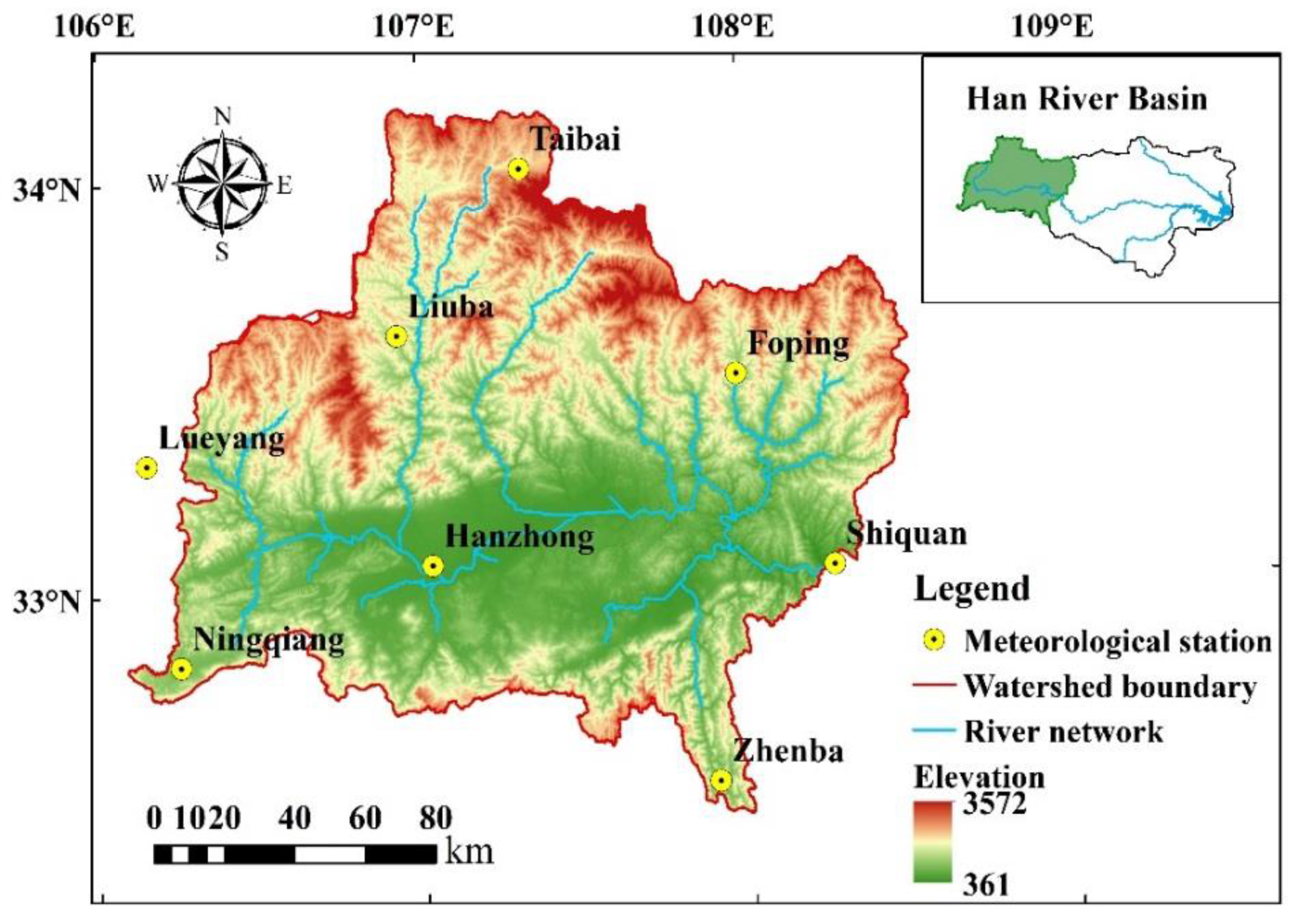
The Han River originates from Ningqiang County, Shaanxi Province of China. The study area is the upstream of Shiquan Hydrological Station in Han River (hereafter named the upper reach of Han River). The upper reach of Han River is located at 106°09′~108°52′ E and 32°45′~34°02′ N, and the catchment area is about 23,750 km2 [38]. The study area is shown in Figure 1.

Figure 1.
The study area.
The landform types above the Shiquan Hydrological Station in the upper reach of the Han River include mountains, hills, plains, and platforms, accounting for 75.24%, 10.24%, 7.86%, and 6.66% of the total area of the basin, respectively. The topographic features are that the north is high and the south is low, Shiquan has the lowest altitude (about 361 m), and Taibai has the highest altitude (about 3572 m).
The study area has a subtropical monsoon climate and there are many subcatchments, which are Yudai River, Hongya River, Taibai River, Youshui River, Ziwu River, and Muma River. The mean annual precipitation is 886 mm, and the precipitation is mainly in the period from July to September. The mean annual PET is 1087 mm. The mean annual runoff is 414 mm at Shiquan station. The mean annual temperature is 13.5 °C, the mean annual minimum temperature is −8.56 °C, and the mean annual maximum temperature is 35.65 °C.
2.2. Data
Meteorological data include daily rainfall, daily maximum temperature, daily maximum minimum temperature, daily average temperature, daily relative humidity, sunshine hours, daily average wind speed, and atmospheric pressure from eight meteorological stations in the study area from 1972 to 2017. The spatial distribution of the meteorological stations is shown in Figure 1, and the station information is shown in Table 1. At the same time, the daily runoff data of Shiquan Hydrological Station from 1972 to 2017 were collected. Meteorological data and measured runoff data were obtained from China Meteorological Data Network and Han River Basin Hydrological Yearbook, respectively.

Table 1.
Meteorological station information in the study area.
The spatial data required in the SWAT model include digital elevation data (DEM), soil data, and land-use data. The DEM data came from the ASTER GDEM 30 m spatial resolution provided by the Geospatial Data Cloud of China. This study adopted the Krasovsky_1940_Albers equal-area conic projection system. The land-use data in 1980, 1995, and 2010 were obtained from the Data Center of Resource and Environmental Sciences, Chinese Academy of Sciences, with a resolution of 1000 m. Soil data were from the World Harmonized Soil Database (HWSD), and the scale is 1:1 million.
3. Methods
3.1. B2015 Function of Generalized Complementary Relationship
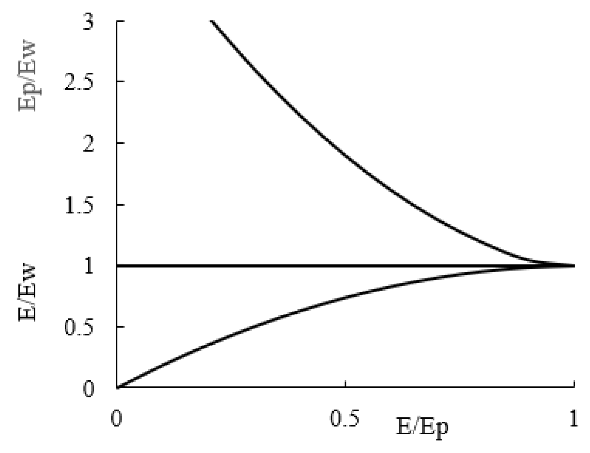
The AA model is the most widely used complementary linear evapotranspiration model. It calculates the potential evapotranspiration through the Penman formula and the humid environment evapotranspiration through the Priestly–Taylor formula. Han et al. [30] carried out dimensionlessization of various complementary evapotranspiration models, and first proposed a nonlinear sigmoid function based on the principle of complementary evapotranspiration (H2012), which corrected the deviation of the AA model under dry and humid conditions. Inspired by the nonlinear complementary model proposed by Han et al. [30], Brutsaert et al. [31] also extended the evapotranspiration complementary relationship model to a dimensionless form , let ,. At the same time, he defined as the actual evapotranspiration, mm/d; is the potential evapotranspiration, mm/d; is the wet environment evapotranspiration rate, mm/d. Use a power function to represent the relationship between and , represent the coefficients in the polynomial.
The B2015 function is based on the following four boundary conditions:
(1) Under completely wet conditions, when , at this time ;
(2) Under extreme drought conditions, when , at this time , is very large;
(3) When, , instant , at this time ;
(4) When the drought situation becomes more and more serious, will be closer to 0 than ; if both reach 0 according to the boundary (2), then for a given increment , the increment will be limited to be smaller, the limit of approaching 0; at this time,.
Through the analysis of the above four boundary conditions, Brutsaert proposed the following quartic polynomial function:
In the formula, is the parameter, −1. The B2015 generalized complementarity is shown in Figure 2.

Figure 2.
B2015 generalized complementarity.
Brutsaert [29] also sorted out the calculation formulas of and in AA model (Brutsaert, 1979) and obtained the expression for calculating the actual evaporation in the basin:
The generalized complementarity relationship can be expressed as follows. It can be seen that the value of decreases with the increase of and increases with the increase of . When the external environment is completely wet,
3.2. SWAT Model
The SWAT model is a distributed watershed hydrological model developed by the Agricultural Research Service of United States Department of Agriculture [44,45]. Developed on the basis of SWRRB (Simulator for Water Resources in Rural Basins) and ROTO (Routing Outputs to The Outlet), it has a good physical foundation. As a widely used hydrological model, it can combine the spatial data provided by GIS and RS (remote sensing) to simulate surface runoff, evapotranspiration, and water quality conditions [46]. Thereby predicting climate change [44], adjustment of land-use measures [47], non-point source pollution and sediment modeling [48,49], the SWAT model is applied to watersheds ranging in size from 102 to 105 km2 in areas with diverse topographic and climatic conditions, including USA, China, Vietnam, Jordan, Australia, South Africa, Brazil, Germany and Switzerland [50], with a wide range of applicability.
The simulated flows in this study were evaluated by the coefficient of determination (R2), Nash–Sutcliffe efficiency coefficient (NSE), Kling–Gupta efficiency (KGE), and relative error (Re).
The coefficient of determination (R2) is used to characterize the change trend between the simulated value and the measured value of the model. When R2 is closer to 1, the simulation is better. The calculation formula is:
where is the simulated value; is the measured value; is the simulated average value; is the measured average value; n is the number of measured values.
The Nash–Sutcliffe efficiency coefficient (NSE) is used to characterize the overall efficiency of the model, and its value is proportional to the reliability of the model. The calculation formula is:
KGE was proposed by Gupta et al. [51] and in optimization, KGE is subject to maximization, with an ideal value at unity.
The relative error is:
3.3. CA–Markov Model
The Markov model quantitatively predicts LULCC in different periods. According to the state of the event at time , it is transformed into the state at time . The state at time is only related to the state at time t [52,53]; the Cellular Automata (CA) model has the concept of spatial information and the ability to simulate dynamic evolution [54]. The Markov model has an absolute advantage in predicting the area of each land-use for a long time in the future, but it cannot predict the changes in the spatial distribution pattern of land use. The CA model can effectively simulate the interaction between cells, and has unique and powerful capabilities in spatial analysis and simulation operations, but there are limitations. The CA–Markov model combines the advantages of Markov and CA spatiotemporal prediction, and can obtain the area-transfer matrix and area transfer probability matrix between land-use states in different periods, which can be used to simulate the spatial change of complex systems and quantitatively predict long time series [55,56]. The formula is as follows [52,57]:
where, i, j = 1,2, …, n respectively represent the types of land use, are elements of the transfer matrix of land-use area, are elements of the transfer probability matrix of land-use area, refers to the time.
3.4. Modeling Framework to Close the Feedback of Evapotranspiration into the Atmosphere Based on Generalized Evapotranspiration Complementary Relationship
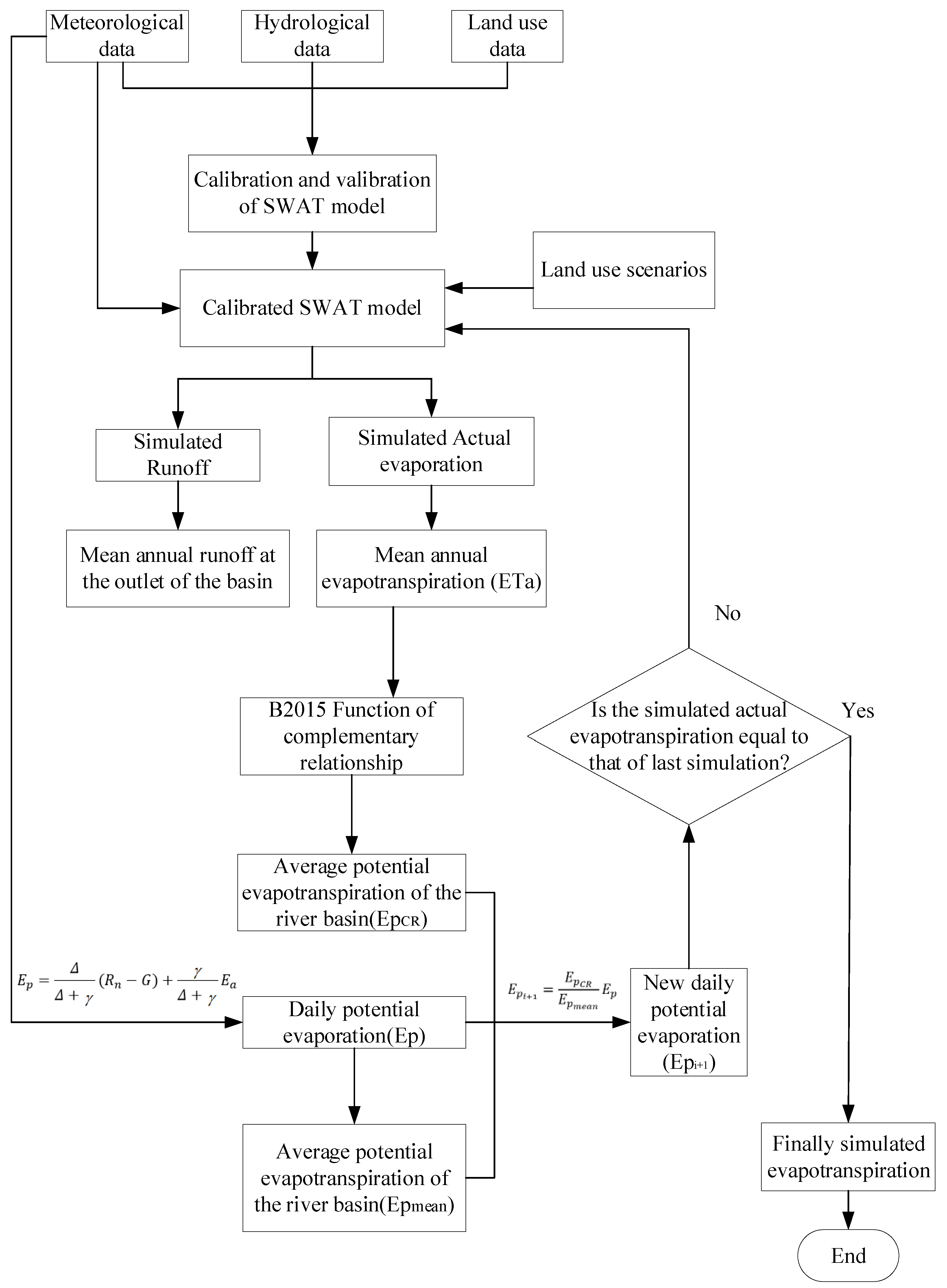
The FCEA based on the generalized evapotranspiration complementary relationship is proposed when predicting the hydrologic response to land-use changes and is shown in Figure 3.
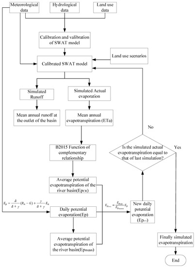
Figure 3.
The modeling framework of iterative calculation of the SWAT model coupled with the evapotranspiration complementary relationship.
The SWAT model is driven by meteorological data and land-use data in the study area, and the evapotranspiration complementary relationship and SWAT model are coupled by AET and PET. Firstly, the calibrated SWAT model was used to simulate the runoff and AET processes, and the daily AET and runoff data of sub basins were obtained. These data were classified, sorted, and weighted to obtain the mean annual actual evapotranspiration (ETa) of the basin. Second, through the generalized evapotranspiration complementary relationship, the average potential evapotranspiration (EPCR) of the basin was calculated from ETa simulated by the SWAT model. Next, the catchment average potential evaporation (Epmean) derived from PET (Ep) calculated from the Penman–Monteith (PM) evapotranspiration formula for each station was used to obtain the corrected potential evaporation (Epi+1) for each station.
They are obtained by correcting the PET according to the following formula:
where: is the average PET of the basin calculated by the evapotranspiration complementary relationship; is the average PET of the basin calculated from meteorological data; is the daily PET calculated of each station calculated by PM evapotranspiration formula; is the corrected daily PET.
Finally, the simulated AET was compared with the last simulated AET. If equal, the final simulated AET was obtained, otherwise the new potential evaporation (Epi+1) was used to drive the SWAT hydrologic model to calculate the AET. This practice was repeated many times until the AET of the last simulation and this simulation tended to be equal, indicating that the feedback of the actual evapotranspiration to the atmosphere reached equilibrium.
4. Estimation of AET in the Upper Reach of the Han River
4.1. Evapotranspiration Complementary Relationship in the Upper Reach of the Han River
The hydrological cycle is a very complex process. In addition to precipitation, evaporation, and runoff, infiltration and interception are also involved. In the hydrological process of the basin, a part of the precipitation forms runoff, which forms observable runoff at the outlet of the basin after routing through the river network. A part of the water returns to the atmosphere through evapotranspiration, and a small part penetrates into the soil. To facilitate the study, only precipitation, runoff, and evapotranspiration in hydrological processes were considered in this study.
In recent years, the principle of evaporation complementarity has been well applied in estimating the AET of the basin. It can estimate the AET with high precision only by using conventional meteorological data. Brutsaert [31] proposed the B2015 function based on the nonlinear generalized complementarity principle. This function was adopted to analyze the complementary relationship of evapotranspiration in this study.
In the study area, the parameters were calibrated using the data of 1972–1990 before the runoff abrupt change based on the water balance method, and the data from 1991–2017 were used for verification. The water balance equation for a closed watershed can be expressed as:
where, P is the annual average precipitation in the watershed, mm; R is the annual average runoff, mm; and ΔW is the change of soil water storage and groundwater in the watershed, mm. At the mean annual scale in the closed watershed, ΔW ≈ 0.
The AET of the basin calculated by water balance equation was used as the observed value and the parameters of B2015 function were calibrated. In the upper reach of Han River, = 0.85, which is the empirical coefficient and the value is affected by factors such as the type of underlying surface, soil water content, distance from the ocean, latitude and longitude, and calculation time scale. Therefore, there is a certain degree of variation in the value of , which needs to be calibrated according to different research areas. The calculated mean annual actual evaporation in 1972–1990 and 1991–2017 was 454.1 mm and 467.1 mm, respectively, and the relative error was 0.92% and −3.69%, respectively, as shown in Table 2. The relative error of the AET estimated by the calibrated B2015 function was less than 5% in both the calibration period and validation period.
Table 2.
AET of the different methods in the upper reach of Han River.
4.2. Catchment Hydrological Modeling without the Feedback
In order to ensure the reliability of the simulation results, the calibration and verification of the model parameters should be carried out in the period when the hydrometeorological sequence is relatively stable. In this study, 1990 was detected as the year of runoff mutation in the study area. The runoff before 1990 was considered as natural runoff, so 1972–1990 was used as the simulation period of the model. 1972–1973 was used as the warm-up period of the model, 1974–1982 was used as the calibration period, and 1983–1990 was used as the validation period.
When the SWAT model was constructed, the land-use index table was established according to the land-use database provided by the model, and it was reclassified. At the same time, the soil classification index table corresponding to the SWAT soil database was established and the soil type raster data were reclassified. The Shiquan station was selected as the outlet of the basin, and the threshold was set to 350 km2 when the sub-watersheds were divided in the SWAT model. The watershed was divided into 35 sub-watersheds. In this study, the thresholds of the three soil layers were set to 10%, 15%, and 10%, respectively, and finally the study area was divided into 249 hydrological response units. Penman method is generally applicable to field-scale evapotranspiration calculation. The reference crop evapotranspiration was used as the external driving force of the atmosphere on the Land Evapotranspiration process to indirectly estimate the actual evapotranspiration. The Penman method was used to calculate the PET, and the daily runoff simulation was carried out in the study area of the upper reach of Han River.
There are many parameters in the SWAT model. Different parameters have different effects on the hydrological process, and the impact on the accuracy of the model simulation results is different. In order to improve the calibration efficiency of the model, it is necessary to carry out parameter sensitivity analysis after the model runs to calibrate and validate the sensitive parameters. This research combined expert advice by the literature and the manual of input and output files of the SWAT model. The 14 parameters that are sensitive to the simulation of the upper reach of Han River basin were selected for model sensitivity analysis, and finally seven sensitive parameters were selected. In SWAT-CUP, after 2000 iterations, the first seven parameters with the highest sensitivity were selected according to the sensitivity from high to low, and then the optimal parameter values were calculated through multiple iterations. The selected runoff sensitive parameters are shown in Table 3. The simulated daily flow at Shiquan hydrological station is shown in Figure 4.
Table 3.
Runoff sensitivity parameters of Shiquan hydrological station.
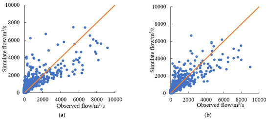
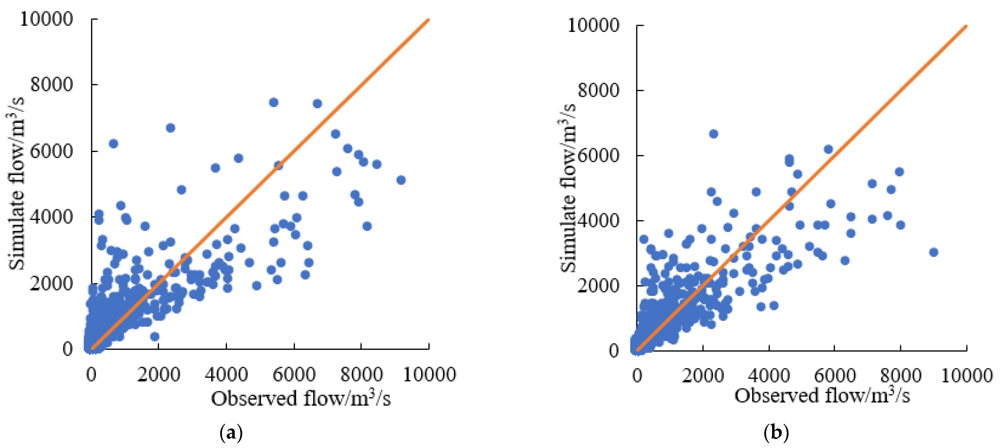
Figure 4.
Simulated daily flow at Shiquan hydrologic station in the calibration and validation periods: (a) calibration period; (b) validation period.
The observed daily flow and the simulated daily flow at Shiquan hydrological station were well fitted, and the evaluation index of simulation results are shown in Table 4. The R2, NSE, and KGE at Shiquan station were above 0.71 in the calibration and validation periods, and the absolution of relative error was within 12.40%. The SWAT model was successfully constructed and had good applicability in the upper reach of Han River. The following analysis is based on the simulation results from 1991 to 2017. We set this as the baseline scenario using the simulation of the 2010 land-use scenario.
Table 4.
Evaluation results of daily runoff simulation at Shiquan hydrological station.
4.3. Evolution Process of Baseline Scenario in the FCEA
In the baseline scenario, the land use data in 2010 were used in the SWAT model, and the daily AET data of the sub-watershed simulated by SWAT model from 1991 to 2017 were obtained. The data of the 27 years were extracted according to the number of sub-watersheds to obtain the matrix of 27 years in 45 sub-watersheds. According to the area weight of each sub-watershed, the annual AET of the whole study area in 27 years was obtained. The mean annual AET of the basin was 500.6 mm.
The B2015 function of complementary relationship was used to calculate the average PET of the basin, and its (EpCR) was 887.9 mm. The average potential evaporation of eight meteorological stations from 1990 to 2017 were calculated by the meteorological data and new daily potential evaporations were calculated as shown in Figure 3.
The new daily potential evaporations were applied to drive the SWAT hydrological model to calculate the AET, and iterate four times. It was found that the AET value of the current simulation and last simulation tended to be 496.3 mm, indicating that the feedback of evapotranspiration to the atmosphere was almost balanced. The AET calculated by water balance equation was 485.5 mm, which was reduced by 2.2% compared with the AET after iteration. It indicates that the current land-use type and climate have tended to be stable, but due to the influence of many complex factors in recent years, it has not reached a complete equilibrium state. Hereafter, the AET will affect the hydrological processes in the upper reach of Han River through the PET that represents the atmosphere-received feedback.
5. Evolution Process of Land-Use Scenario in the FCEA
5.1. Land-Use Scenarios
Based on the land-use data of the study area in 2010 and the meteorological data from 1991 to 2017, this study set it as the baseline scenario. Based on the change characteristics of land use in 1980 and 1995, four land-use scenarios were set up to explore the changes of mean annual runoff and evapotranspiration in different land-use scenarios.
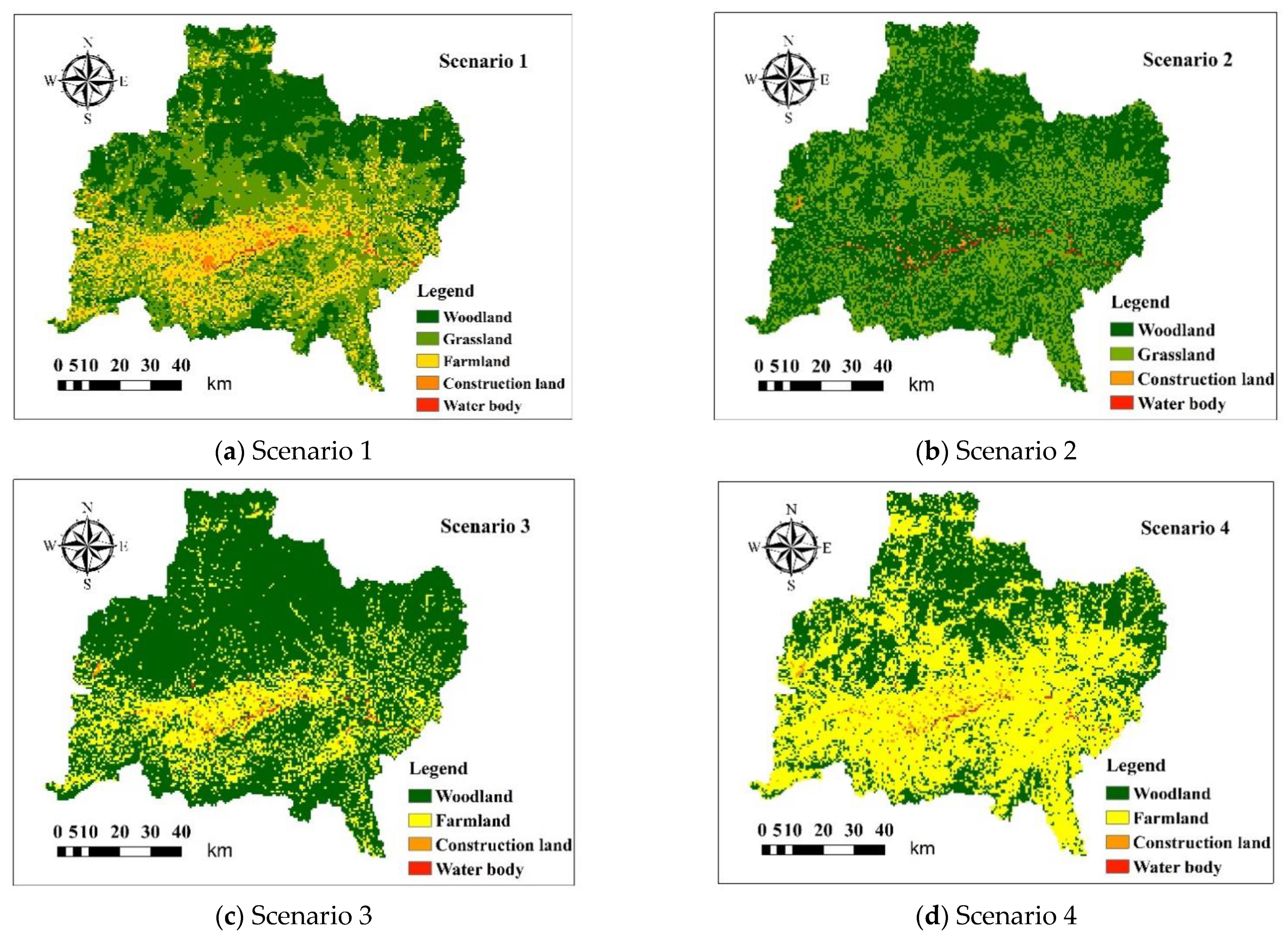
In Scenario 1, it was assumed that the future land use in the study area will continue to evolve according to the past trend. Based on the land-use data in 1995 and 2010, the step of the transfer matrix is 15 years and the CA–Markov model combined with GIS software was used to predict the land use in the study area in 2025. The land-use transfer matrix of the study area in different years was obtained in the IDRISI, and the land use in 2025 was predicted in the CA–Markov model.
In order to evaluate the simulation result of the CA–Markov model in the study area, the land-use data in 1980 and 1995 were used in the CA–Markov model to simulate the land use in 2010. The simulated land use was compared with the actual land-use map in 2010 to evaluate the simulated result. Generally, the Kappa coefficient is used to evaluate the accuracy of remote sensing data spatial simulation, the Kappa coefficient of the land-use map in 2010 and simulated by the CA–Markov model was 0.91, indicating that the model simulation has high prediction accuracy and can be used to simulate and predict land use in 2025. Therefore, the land use of the study area in 2025 was simulated and predicted, which is Scenario 1. The results showed that the woodland increased by 14 km2, the farmland decreased by 123 km2, the grassland increased by 18 km2, the construction land increased by 64 km2, and the water area increased by 27 km2.
In Scenario 2, the farmland in the study area was transformed into woodland. The result is that the woodland increased by 5818 km2 and the farmland decreased by 5818 km2.
In Scenario 3, the grassland in the study area was transformed into woodland. The result is that the woodland increased by 8598 km2 and the grassland decreased by 8598 km2.
In Scenario 4, the grassland in the study area is transformed into farmland, the result is that the farmland increases by 8598 km2 and the grassland decreases by 8598 km2.
The area of land use in different scenarios is shown in Table 5. The results of land use in the study area are shown in Figure 5. The study area of the upper reach of Han River are mainly woodland, grassland and farmland, which account for more than 98% of the whole area. The area of woodland decreased from 1980 to 1995 and increased from 1995 to 2010. The grassland increased before 1995, and the area has decreased since then. The area of farmland decreased from 1980 to 1995. The area of construction land and water body decreased slightly from 1980 to 1995, and from 1995 to 2010, the area increased significantly. From 1980 to 2010, the change of land use in the study area mainly occurred among woodland, grassland, and farmland.
Table 5.
Area of land-use type in each scenario.

Figure 5.
Spatial change map of land use under each scenario.
5.2. Analysis of Simulated Runoff in Different Scenarios
It is assumed that the precipitation remains unchanged, and the long-term evolution of runoff in different scenarios are simulated in FCEA, and the feedback of actual evaporation to the atmosphere is realized based on the complementary relationship of evaporation. Some former studies on the hydrological effects of the afforestation emphasized that runoff and soil moisture in temperate regions decreased due to increased AET [58]. In terms of watershed water balance, under the condition of long-term evolution, when the precipitation input in the model (the area-weighted average of annual precipitation at all stations is 838.3 mm) remains unchanged, the AET decreases and the runoff increases.
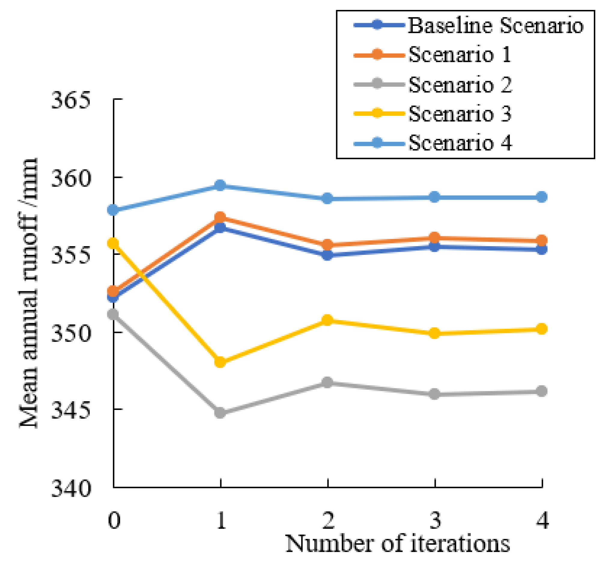
The mean annual simulated runoff of each iteration in the baseline scenario and four scenarios are shown in Table 6 and Figure 6. The mean annual simulated runoff was 352.2 mm in the baseline scenario (land use in 2010) in the initial simulation.
Table 6.
Simulated runoff of multiple iterations in each scenario.
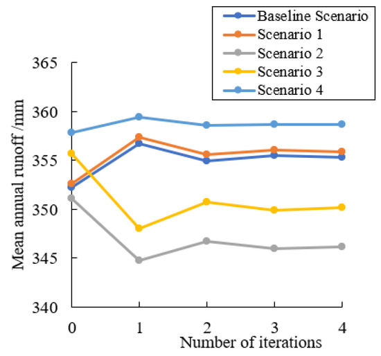
Figure 6.
Changes of simulated runoff in all simulations in different scenarios.
The mean annual runoff in Scenario 1 had a little change, which increased by 0.10% in the initial simulation compared with the runoff in the baseline scenario. With the long-term interaction of the atmosphere, the feedback of evapotranspiration increased the runoff to 355.9 mm in Scenario 1.
The conversion of farmland into woodland in Scenario 2 reduced the runoff by 0.33% in initial simulation compared with the baseline scenario, but the watershed runoff under the feedback of long-term evapotranspiration decreased by 2.55% in the final simulation compared with the baseline scenario. In Scenario 3, grassland was transformed into woodland, which increased by 0.98% in the initial simulation compared with the simulated runoff in the baseline scenario, but the watershed runoff under the feedback of long-term evapotranspiration decreased by 1.45% in the final simulation compared with the baseline scenario. In Scenario 4, grassland is transformed into farmland, which increased by 1.58% in the initial simulation compared with the simulated runoff in the baseline scenario, and the watershed runoff under the feedback of long-term evapotranspiration increased by 0.94% in the final simulation compared with the baseline scenario. As shown in Figure 6, the trends of the runoff changes from the initial simulation to the second simulation were all different from those from the second simulation to the third simulation. The simulated runoff in the fourth simulation was almost equal to that in the third simulation in all 5 scenarios. In the trends of the final simulation, the simulated runoff in Scenario 4 was the maximum and that in Scenario 2 was the minimum.
5.3. Analysis of Simulated Evapotranspiration in Different Scenarios
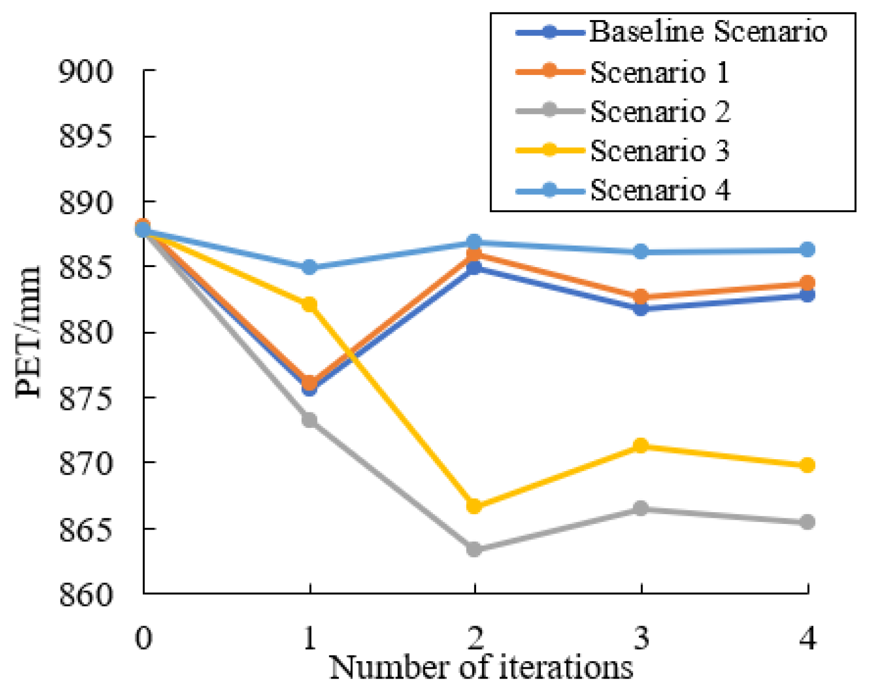
Mean annual potential evaporation and mean annual evapotranspiration after multiple iterations in four scenarios are shown in Table 7 and Table 8. The PET in the final simulation was smaller than the PET in the initial simulation in the four scenarios we set up earlier.The AET in the final simulation was smaller than the PET in the initial simulation in the baseline scenario, Scenario 1, and Scenario 4, and was larger in Scenarios 2 and 3. The changes of the PET of every iteration under different scenarios are shown in Figure 7, and the changes of AET of every iteration under different scenarios are shown in Figure 8.
Table 7.
Annual potential evaporation in multiple iterations in each scenario.
Table 8.
Simulated annual evapotranspiration of multiple iterations in each scenario.
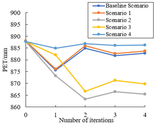
Figure 7.
Annual PET input in the SWAT model from the complementary relationship in different scenarios.
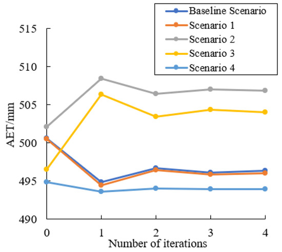
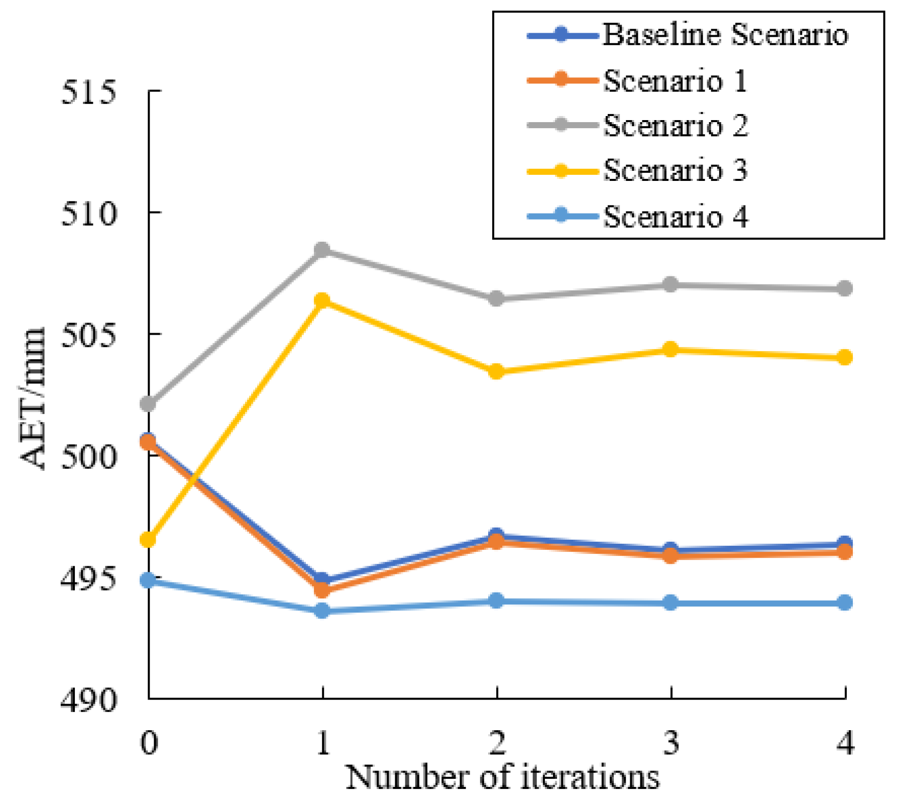
Figure 8.
Simulated annual AET from the SWAT model in different scenarios.
Compared with the baseline scenario, the input PET and output AET of the hydrological simulation changed a little in Scenario 1, i.e., natural growth scenario, indicating that the evapotranspiration in the basin almost reached a stable state under the natural change condition.
In Scenario 2, the conversion of farmland to woodland increased by 0.30% compared with the AET in initial simulation in the baseline scenario, but the AET under the long-term evapotranspiration feedback increased by 2.12% in the final simulation compared with the baseline scenario.
In Scenario 3, grassland is converted into woodland. Compared with the AET of the baseline scenario, the AET in the initial simulation decreased by 0.81%, and the AET in the final simulation after the long-term evapotranspiration feedback increased by 1.56% compared with the baseline scenario.
In Scenario 4, the conversion of grassland into farmland reduced the AET by 1.15% in the initial simulation compared with the baseline scenario, and the AET in the final simulation after the long-term evapotranspiration feedback was reduced by 0.48% compared with the baseline scenario.
The results of Scenario 2 and Scenario 3 indicate that the increase of woodland will increase the AET of the watershed after the long-term evapotranspiration feedback, and the result of Scenario 4 indicates that the conversion of grassland to farmland will reduce the AET of the watershed after long-term feedback.
6. Discussion
In previous studies, scholars used conventional meteorological data to estimate the actual evaporation through the generalized nonlinear complementary relationship of evaporation [26,27,28,29,30,31,32,33]. Usually, they used different boundary conditions and different ideas to analyze the influence of land surface moisture conditions. The models improved by the AA model all use the , as does the B2015 function used in this article. At present, α, as an atmospheric characteristic parameter, represents the influence of the Priestly–Taylor coefficient and surface dry and wet state, and is related to advection, aerodynamic conditions, etc. [59]. In this study, the constant parameter was used for different land-use scenarios, and the impact of land-use change on the complementary relationship parameter was not considered. This may have some impact on the simulation results. In the future, the parameter α can be determined according to different land-use scenarios, and the impact of the calibrated parameter under different land-use scenarios on the simulated runoff and AET can be analyzed.
The objective of this study was to close the feedback of evapotranspiration into the atmosphere based on the evapotranspiration complementary relationship in the catchment hydrological modeling, and simulate the effect of land-use changes on the runoff and evapotranspiration. The purpose of this study was to simulate the impact of land-use change on runoff and evapotranspiration based on the complementary relationship of evapotranspiration in the hydrological model of the basin, close the feedback of evapotranspiration to the atmosphere. One of the steps of the iterative simulation method used in the study is as follows: after correcting the weighted average value calculated by each hydrological station in the basin, the potential evapotranspiration of the whole basin was taken as a whole input for the model. To some extent, there is still room for improvement in such calculation results. The potential evapotranspiration of the whole basin was the input for the model, and each sub basin was allocated through the model. This model depends on the structure of the hydrological model. The iterative simulation was completed by the distributed SWAT model. Its own potential evapotranspiration input function hinders the further development of this work. In future work, we will try to couple multiple hydrological models, input different PET for different sub basins into different PET, further refine the intermediate iteration work, and optimize the framework to close the feedback of evapotranspiration to the atmosphere.
7. Conclusions
In this study, FCEA based on the evapotranspiration complementary relationship was proposed in the catchment hydrological modeling, and the effect of land-use changes on the runoff and evapotranspiration in the upper reach of Han River of China were investigated in the FCEA.
In the framework, the SWAT model was established in the study area, and the evapotranspiration complementary relationship was verified. To close the feedback of watershed evapotranspiration to the atmosphere, the evapotranspiration complementary relationship was coupled to the SWAT model. The PET calculated by the complementary relationship from the AET simulated by the SWAT model was used as the input of the SWAT model. After several iterations, the AET of the simulation tended to be equal with that of last simulation, which indicates that the feedback of evapotranspiration to the atmosphere reached a balance. The impacts of evapotranspiration feedback on runoff in the basin in four land-use scenarios were analyzed, and the runoff response and evapotranspiration changes were discussed.
Based on the data of 1972–2017, the B2015 function of the evapotranspiration complementary relationship in the study area was calibrated to obtain = 0.85, and the AET in the study area was estimated based on the water balance and the evapotranspiration complementary relationship. The SWAT model was calibrated and validated in the study area in 1972–1990. The simulation results of daily runoff at Shiquan hydrological station in the calibration and validation periods were evaluated. All of R2, NSE, and KGE were greater than 0.71, and the absolution of Re was smaller than 12.40%.
The iteration simulation results of the baseline scenario showed that, when the feedback of evapotranspiration to the atmosphere reached a balance, the runoff change caused by the natural increase of land use was small compared with the initial simulation. In baseline scenario, Scenario 1, and Scenario 4, the runoff in the final simulation increased compared with the initial simulation. In Scenarios 2 and 3, the runoff did not increase as the woodland area increased. If the precipitation remains stable, increasing the woodland will not achieve the effect of increasing the runoff of the watershed. It is shown that the increase of the forest area will increase the runoff in the short term, but in the process of long-term coupling with the atmosphere, the increase of the forest area will lead to an increase in evaporation and a decrease in runoff. The study also shows that if some grassland is converted into farmland, the runoff of the watershed will increase, which should be considered in land-use planning. The results can provide some theoretical support for the ecological governance of the Han River basin and the protection of water source region of trans-boundary water transfer projects in the Han River basin. According to the 2006–2020 Land Use Planning of Shaanxi Province and the 14th Five-Year Plan of Shaanxi Province, the planning requires the forest coverage rate in upper reach of Han River to reach more than 46.5%. The upper reach of the Han River is a key ecological protection area in China. The planning also proposes to effectively protect the ecological environment and basic farmland in the study area, and implement the strictest land-saving system for construction land. If the land use in the future follows the pattern of increasing woodland and farmland, the runoff of the river basin will not increase after the long-term feedback. The increase of woodland will increase the evapotranspiration of the river basin and reduce the runoff when the long-term precipitation remains stable. Because of the influence of various factors, the formulation of land-use planning policy is difficult in the sustainable development of the Han River.
Author Contributions
Conceptualization, T.L., D.L, S.H. and G.M.; methodology, T.L., D.L. and S.H.; software, T.L. and D.L.; validation, T.L. and D.L.; formal analysis, T.L., D.L. and S.H.; investigation, T.L. and D.L.; resources, T.L. and D.L.; data curation, T.L. and D.L.; writing—original draft, T.L., D.L., S.H. and G.M.; writing—review and editing, T.L., D.L., S.H., G.M., J.F., X.M. and Q.H.; visualization, T.L. and D.L.; supervision, D.L.; project administration, D.L. All authors have read and agreed to the published version of the manuscript.
Funding
This study was partially supported by the National Natural Science Foundation of China (NSFC) (Grant Nos. 42071335, 52109031 and 51979252), State Key Laboratory of Eco-hydraulics in Northwest Arid Region, China (Grant No. 2019KFKT-4) and Natural Science Basic Research Program of Shaanxi-Han to Wei Water Transfer Joint Foundation (2022JC-LHJJ-13).
Institutional Review Board Statement
Not applicable.
Informed Consent Statement
Not applicable.
Data Availability Statement
Not applicable.
Acknowledgments
This study was partially supported by the National Natural Science Foundation of China (NSFC) (Grant Nos. 42071335, 52109031 and 51979252), State Key Laboratory of Eco-hydraulics in Northwest Arid Region, China (Grant No. 2019KFKT-4) and Natural Science Basic Research Program of Shaanxi-Han to Wei Water Transfer Joint Foundation(2022JC-LHJJ-13). The authors thank the editor and anonymous reviewers for their constructive comments.
Conflicts of Interest
The authors declare no conflict of interest. The funders had no role in the design of the study; in the collection, analyses, or interpretation of data; in the writing of the manuscript, or in the decision to publish the results.
References
- Allen, M.R.; Ingram, W.J. Constraints on future changes in climate and the hydrologic cycle. Nature 2002, 419, 228–232. [Google Scholar] [CrossRef] [PubMed]
- Taikan, O.; Shinjiro, K. Global Hydrological Cycles and World Water Resources. Science 2006, 313, 1068–1072. [Google Scholar]
- Allen, M.; Babiker, M.; Chen, Y.; Taylor, M.; Tschakert, P.; Waisman, H.; Zhai, P. Summary for Policymakers. In Global Warming of 1.5 °C: An IPCC Special Report; Cambridge University Press: Cambridge, UK; New York, NY, USA, 2018. [Google Scholar]
- Wilfried, B. Global land surface evaporation trend during the past half century: Corroboration by Clausius-Clapeyron scaling. Adv. Water Resour. 2017, 106, 3–5. [Google Scholar]
- Trenberth, K.E.; Smith, L.; Qian, T.; Dai, A.; Fasullo, J. Estimates of the Global Water Budget and Its Annual Cycle Using Observational and Model Data. J. Hydrometeorol. 2007, 8, 758–769. [Google Scholar] [CrossRef]
- Trenberth, K.E.; Fasullo, J.T.; Kiehl, J. Earth’s global energy budget. B Am. Meteorol. Soc. 2009, 90, 311–324. [Google Scholar] [CrossRef]
- Liu, X.; Li, Y.; Chen, X.; Zhou, G.; Cheng, J.; Zhang, D.; Meng, Z.; Zhang, Q. Partitioning evapotranspiration in an intact forested watershed in southern China. Ecohydrology 2015, 8, 1037–1047. [Google Scholar] [CrossRef]
- Sun, S.K.; Li, C.; Wang, Y.B.; Zhao, X.N.; Wu, P.T. Evaluation of the mechanisms and performances of major satellite-based evapotanspiration models im Northwest China. Agric. Forest Meteorol. 2020, 291, 108056. [Google Scholar] [CrossRef]
- Lian, X.; Piao, S.; Huntingford, C.; Li, Y.; Zeng, Z.; Wang, X.; Ciais, P.; McVicar, T.R.; Peng, S.; Ottlé, C.; et al. Partitioning global land evapotranspiration using CMIP5 models constrained by observations. Nat. Clim. Change 2018, 8, 640–646. [Google Scholar] [CrossRef]
- Neitsch, S.L.; Arnold, J.G.; Kiniry, J.R. Soil and Water Assessment Tool Theoretical Documentation Version 2009; Texas Water Resources Institute: College Station, TX, USA, 2011. [Google Scholar]
- Yuan, L.; Ma, Y.; Chen, X.; Wang, Y.; Li, Z. An enhanced MOD16 evapotranspiration model for the Tibetan Plateau during the unfrozen season. J. Geophys. Res. Atmos. 2021, 126, e2020JD032787. [Google Scholar] [CrossRef]
- Liang, W.; Bai, D.; Wang, F.; Fu, B.; Yan, J.; Wang, S.; Yang, Y.; Long, D.; Feng, M. Quantifying the impacts of climate change and ecological restoration on streamflow changes based on a Budyko hydrological model in China’s Loess Plateau. Water Resour. Res. 2015, 51, 6500–6519. [Google Scholar] [CrossRef]
- You, G.; Arain, M.A.; Wang, S.; Lin, N.; Wu, D.; McKenzie, S.; Zou, C.; Liu, B.; Zhang, X.; Gao, J. Trends of actual and potential evapotranspiration based on Bouchet’s complementary concept in a cold and arid steppe site of Northeastern Asia. Agric. For. Meteorol. 2019, 279, 107684. [Google Scholar]
- Liu, C.; Zhang, D.; Liu, X.; Zhao, C. Spatial and temporal change in the potential evapotranspiration sensitivity to meteorological factors in China (1960–2007). J. Geogr. Sci. 2012, 22, 3–14. [Google Scholar]
- Fohrer, N.; Haverkamp, S.; Eckhardt, K.; Frede, H.G. Hydrologic Response to land use changes on the catchment scale. Phys. Chem. Earth. Part B Hydrol. Ocean. Atmos. 2001, 26, 577–582. [Google Scholar] [CrossRef]
- Ershadi, A.; McCabe, M.F.; Evans, J.P.; Wood, E.F. Impact of model structure and parameterization on Penman–Monteith type evaporation models. J. Hydrol. 2015, 525, 521–535. [Google Scholar]
- Ozdogan, M.; Salvucci, G.D. Irrigation-induced changes in potential evapotranspiration in southeastern Turkey; test and application of Bouchet’s complementary hypothesis. Water Resour. Res. 2004, 40, W4301. [Google Scholar]
- Yang, X.; Ren, L.; Singh, V.P.; Liu, X.; Yuan, F.; Jiang, S.; Yong, B. Impacts of land use and land cover changes on evapotranspiration and runoff at Shalamulun River watershed, China. Hydrol. Res. 2012, 43, 23–37. [Google Scholar] [CrossRef]
- Han, J.; Zhao, Y.; Wang, J.; Zhang, B.; Zhu, Y.; Jiang, S.; Wang, L. Effects of different land use types on potential evapotranspiration in the Beijing-Tianjin-Hebei region, North China. J. Geogr. Sci. 2019, 29, 922–934. [Google Scholar] [CrossRef]
- Fisher, J.B.; Melton, F.; Middleton, E.; Hain, C.; Anderson, M.; Allen, R.; McCabe, M.F.; Hook, S.; Baldocchi, D.; Townsend, P.A.; et al. The future of evapotranspiration: Global requirements for ecosystem functioning, carbon and climate feedbacks, agricultural management, and water resources. Water Resour. Res. 2017, 53, 2618–2626. [Google Scholar]
- Peng, L.; Zeng, Z.; Wei, Z.; Chen, A.; Wood, E.F.; Sheffield, J. Determinants of the ratio of actual to potential evapotranspiration. Global Change Biol. 2019, 25, 1326–1343. [Google Scholar] [CrossRef]
- Senay, G.B.; Kagone, S.; Velpuri, N.M. Operational Global Actual Evapotranspiration: Development, Evaluation, and Dissemination. Sensors 2020, 20, 1915. [Google Scholar]
- McMahon, T.A.; Finlayson, B.L.; Peel, M.C. Historical developments of models for estimating evaporation using standard meteorological data. Wiley Interdiscip. Rev. Water 2016, 3, 788–818. [Google Scholar]
- Han, S.; Tian, F. A review of the complementary principle of evaporation: From the original linear relationship to generalized nonlinear functions. Hydrol. Earth Syst. Sc. 2020, 24, 2269–2285. [Google Scholar]
- Zhang, L.; Cheng, L.; Brutsaert, W. Estimation of land surface evaporation using a generalized nonlinear complementary relationship. J. Geophys. Res. Atmos. 2017, 122, 1475–1487. [Google Scholar]
- Han, S.; Tian, F. Derivation of a Sigmoid Generalized Complementary Function for Evaporation With Physical Constraints. Water Resour. Res. 2018, 54, 5050–5068. [Google Scholar]
- Bouchet, R. Evapotranspiration reelle at potentielle, signification climatique. Int. Assoc. Sei. Hydro. Pub. 1963, 62, 134–142. [Google Scholar]
- Li, Y.; Piao, S.; Li, L.Z.X.; Chen, A.; Wang, X.; Ciais, P.; Huang, L.; Lian, X.; Peng, S.; Zeng, Z.; et al. Divergent hydrological response to large-scale afforestation and vegetation greening in China. Sci. Adv. 2018, 4, eaar4182. [Google Scholar]
- Brutsaert, W.; Stricker, H. An advection-aridity approach to estimate actual regional evapotranspiration. Water Resour. Res. 1979, 15, 443–450. [Google Scholar]
- Han, S.; Hu, H.; Tian, F. A nonlinear function approach for the normalized complementary relationship evaporation model. Hydrol. Process. 2012, 26, 3973–3981. [Google Scholar]
- Brutsaert, W. A generalized complementary principle with physical constraints for land-surface evaporation. Water Resour. Res. 2015, 51, 8087–8093. [Google Scholar] [CrossRef]
- Szilagyi, J.; Crago, R.; Qualls, R. A calibration-free formulation of the complementary relationship of evaporation for continental-scale hydrology. J. Geophys. Res. Atmos. 2017, 122, 264–278. [Google Scholar]
- Crago, R.D.; Qualls, R.J. Evaluation of the Generalized and Rescaled Complementary Evaporation Relationships. Water Resour. Res. 2018, 54, 8086–8102. [Google Scholar]
- Xu, X.; Li, X.; Wang, X.; He, C.; Tian, W.; Tian, J.; Yang, L. Estimating daily evapotranspiration in the agricultural-pastoral ecotone in Northwest China: A comparative analysis of the Complementary Relationship, WRF-CLM4.0, and WRF-Noah methods. Sci. Total Environ. 2020, 729, 138635. [Google Scholar] [PubMed]
- Zhou, H.; Han, S.; Liu, W. Evaluation of two generalized complementary functions for annual evaporation estimation on the Loess Plateau, China. J. Hydrol. 2020, 587, 124980. [Google Scholar]
- Kim, D.; Chun, J.A.; Ko, J. A hybrid approach combining the FAO-56 method and the complementary principle for predicting daily evapotranspiration on a rainfed crop field. J. Hydrol. 2019, 577, 123941. [Google Scholar]
- Zhang, W.; Zhang, Z.; Wei, X.; Hu, Y.; Li, Y.; Meng, L. Long-term spatiotemporal changes of surface water and its influencing factors in the mainstream of Han River, China. J. Hydrol. Reg. Stud. 2022, 40, 101009. [Google Scholar]
- Jiang, Z.; Jiang, W.; Ling, Z.; Wang, X.; Peng, K.; Wang, C. Surface Water Extraction and Dynamic Analysis of Baiyangdian Lake Based on the Google Earth Engine Platform Using Sentinel-1 for Reporting SDG 6.6.1 Indicators. Water 2021, 13, 138. [Google Scholar]
- Wang, C.; Jia, M.; Chen, N.; Wang, W. Long-Term Surface Water Dynamics Analysis Based on Landsat Imagery and the Google Earth Engine Platform: A Case Study in the Middle Yangtze River Basin. Remote Sens. 2018, 10, 1635. [Google Scholar]
- Hu, Q.; Cao, S.; Yang, H.; Wang, Y.; Li, L.; Wang, L. Daily runoff predication using LSTM at the Ankang Station, Hanjing River. Prog. Geogr. 2020, 39, 4000636. [Google Scholar]
- Tan, L.; Cai, Y.; Cheng, H.; Edwards, L.R.; Gao, Y.; Xu, H.; Zhang, H.; An, Z. Centennial-to decadal-scale monsoon precipitation variations in the upper Hanjiang River region, China over the past 6650 years. Earth Planet. Sc. Lett. 2018, 482, 580–590. [Google Scholar]
- Stannard, D.I. Comparison of Penman-Monteith, Shuttleworth-Wallace, and Modified Priestley-Taylor Evapotranspiration Models for wildland vegetation in semiarid rangeland. Water Resour. Res. 1993, 29, 1379–1392. [Google Scholar]
- Vörösmarty, C.J.; Federer, C.A.; Schloss, A.L. Potential evaporation functions compared on US watersheds: Possible implications for global-scale water balance and terrestrial ecosystem modeling. J. Hydrol. 1998, 207, 147–169. [Google Scholar]
- Binod, B.; Sangam, S.; Pallav, K.S.; Rocky, T. Evaluation and application of a SWAT model to assess the climate change impact on the hydrology of the Himalayan River Basin. Catena 2019, 181, 104082. [Google Scholar]
- Maysara, G.; Zhong, L. Propagation of parameter uncertainty in SWAT: A probabilistic forecasting method based on polynomial chaos expansion and machine learning. J. Hydrol. 2020, 586, 124854. [Google Scholar]
- Amirhossein, S.T.; Giancarlo, H.C.; Hamideh, N.; Sina, A. River basin-scale flood hazard assessment using a modified multi-criteria decision analysis approach: A case study. J. Hydrol. 2019, 574, 660–671. [Google Scholar]
- Chen, L.; Chen, S.; Li, S.; Shen, Z. Temporal and spatial scaling effects of parameter sensitivity in relation to non-point source pollution simulation. J. Hydrol. 2019, 571, 36–49. [Google Scholar]
- Yang, S.; Dong, G.; Zheng, D.; Xiao, H.; Gao, Y.; Lang, Y. Coupling Xinanjiang model and SWAT to simulate agricultural non-point source pollution in Songtao watershed of Hainan, China. Ecol. Model. 2011, 222, 3701–3717. [Google Scholar]
- Pinto, D.B.F.; Da, S.A.M.; Beskow, S.; De Mello, C.R.; Coelho, G. Application of the Soil and Water Assessment Tool (SWAT) for Sediment Transport Simulation at a Headwater Watershed in Minas Gerais State, Brazil. Trans. ASABE 2013, 56, 697–709. [Google Scholar]
- Douglas-Mankin, K.R.; Srinivasan, R.; Arnold, J.G. Soil and Water Assessment Tool (SWAT) Model: Current Developments and Applications. Trans. ASABE 2010, 53, 1423–1431. [Google Scholar] [CrossRef]
- Gupta, H.V.; Kling, H.; Yilmaz, K.K.; Martinez, G.F. Decomposition of the mean squared error and NSE performance criteria: Implications for improving hydrological modelling. J. Hydrol. 2009, 377, 80–91. [Google Scholar]
- Behera, M.D.; Borate, S.N.; Panda, S.N.; Behera, P.R.; Roy, P.S. Modelling and analyzing the watershed dynamics using Cellular Automata (CA)-Markov model - A geo-information based approach. J. Earth Syst. Sci. 2012, 121, 1011–1024. [Google Scholar]
- Losiri, C.; Nagai, M.; Ninsawat, S.; Shrestha, R.P. Modeling Urban Expansion in Bangkok Metropolitan Region Using Demographic–Economic Data through Cellular Automata-Markov Chain and Multi-Layer Perceptron-Markov Chain Models. Sustainability 2016, 8, 686. [Google Scholar]
- Zhou, C.H.; Ou, Y.; Ma, T.; Qin, B. Theoretical perspectives of CA-based geographical system modeling. Prog. Geogr. 2009, 28, 833–838. [Google Scholar]
- Ghosh, P.; Mukhopadhyay, A.; Chanda, A.; Mondal, P.; Akhand, A.; Mukherjee, S.; Nayak, S.K.; Ghosh, S.; Mitra, D.; Ghosh, T.; et al. Application of Cellular automata and Markov-chain model in geospatial environmental modeling-A review. Remote Sens. Appl. Soc. Environ. 2017, 5, 64–77. [Google Scholar]
- Fu, F.; Liu, W.; Wu, D.; Deng, S.; Bai, Z. Research on the Spatiotemporal Evolution of Land Use Landscape Pattern in a County Area Based on CA-Markov Model. Sustain. Cities Soc. 2022, 80, 103760. [Google Scholar]
- Ongsomwang, S.; Pimjai, M. Land use and land cover prediction and its impact on surface runoff. Suranaree J. Sci. Technol. 2015, 22, 205–223. [Google Scholar]
- Brown, A.E.; Zhang, L.; McMahon, T.A.; Western, A.W.; Vertessy, R.A. A review of paired catchment studies for determining changes in water yield resulting from alterations in vegetation. J. Hydrol. 2004, 310, 28–61. [Google Scholar] [CrossRef]
- Han, S.; Tian, F.; Wang, W.; Wang, L. Sigmoid generalized complementary equation for evaporation over wet surfaces: A nonlinear modification of the Priestley-Taylor equation. Water Resour. Res. 2021, 57, e2020WR028737. [Google Scholar]
Publisher’s Note: MDPI stays neutral with regard to jurisdictional claims in published maps and institutional affiliations. |
© 2022 by the authors. Licensee MDPI, Basel, Switzerland. This article is an open access article distributed under the terms and conditions of the Creative Commons Attribution (CC BY) license (https://creativecommons.org/licenses/by/4.0/).