Tuning ANN Hyperparameters by CPSOCGSA, MPA, and SMA for Short-Term SPI Drought Forecasting

Abstract

Modelling drought is vital to water resources management, particularly in arid areas, to reduce its effects. Drought severity and frequency are significantly influenced by climate change. In this study, a novel hybrid methodology was built, data preprocessing and artificial neural network (ANN) combined with the constriction coefficient-based particle swarm optimisation and chaotic gravitational search algorithm (CPSOCGSA), to forecast standard precipitation index (SPI) based on climatic factors. Additionally, the marine predators algorithm (MPA) and the slime mould algorithm (SMA) were used to validate the performance of the CPSOCGSA algorithm. Climatic factors data from 1990 to 2020 were employed to create and evaluate the SPI 1, SPI 3, and SPI 6 models for Al-Kut City, Iraq. The results indicated that data preprocessing methods improve data quality and find the best predictors scenario. The performance of CPSOCGSA-ANN is better than MPA-ANN and SMA-ANN algorithms based on various statistical criteria (i.e., R², MAE, and RMSE). The proposed methodology yield R² = 0.93, 0.93, and 0.88 for SPI 1, SPI 3, and SPI 6, respectively.

1. Introduction

Drought is one of the most devastating natural catastrophes globally, causing the highest economic losses, and it happens when there is a shortage of precipitation compared to the long-term average precipitation [1,2]. On a worldwide scale, drought is responsible for 22% of the economic losses caused by calamities and 33% of the losses in terms of the number of people affected [3,4]. There are four types of droughts: meteorological, agricultural, socioeconomic, and hydrological [5]. Drought is dependent on climatic variables such as rainfall and temperature. Additionally, there are a variety of drought indicators available, such as the Palmer drought severity index (PDSI), standardised precipitation evapotranspiration index (SPEI), effective drought index (EDI), reconnaissance drought index (RDI), and standardised precipitation index (SPI). SPI was introduced by McKee, et al. [6], which is the most widely employed drought indicator and has been recommended by the World Meteorological Organisation [7]. The SPI can be computed at various timescales to provide insight into various types of drought; for example, the short-to-medium timescale is appropriate for agricultural and meteorological droughts [8].

Climate change is causing significant issues for the ecosystem, such as rainfall variation, which may lead to drought and desertification [9,10]. Additionally, the effect of global warming on temperature and precipitation in various areas of the world is uneven. The Arabian Peninsula, which has a mostly desert environment, is expected to face more rapid climate change due to global warming [11].

Iraq, an arid country on the Arabian Peninsula, is one of the most affected by climate change in the world [12,13]. The Tigris and the Euphrates rivers are Iraq’s most important freshwater sources. As a result, many storage dams have been built along the paths of these rivers in Iraq [14]. These rivers had severe water shortages from 2009 to 2014, which are predicted to increase due to climate change, leading to a rise in upstream water consumption (i.e., Turkey and Iran) [14,15]. Climate change has significant effects in Iraq, such as decreasing rainfall and increasing temperatures [16]. Osman, et al. [17] showed that most Iraqi areas are expected to experience decreased annual mean rainfall, particularly towards the end of the twenty-first century. Additionally, Salman, et al. [11] deduced that yearly precipitation is decreasing at a rate of −1.0 to −5.0 mm/year in northwest Iraq. Furthermore, the temperature of Iraq is rising at a rate two to seven times more rapidly than the world average [12]. As a result, these studies highlight the need for more research in drought forecasting in Iraq. It plays a significant role in providing decision-makers with helpful information that enables them to make appropriate decisions to alleviate the effects of drought [18,19].

Drought forecasting is essential for irrigated agriculture, water management, environmental monitoring, recreational tourism, and ecosystem health [20]. Additionally, drought prediction and early warning are important for agricultural adaptability to climate change [21]. Various machine learning (ML) technologies have shown remarkable performance in forecasting droughts due to their ability to manage the nonlinear correlation between meteorological factors and drought [22,23]. Traditional methods assume that the relationship between the predictors and the predictand is linear and may be unsuitable for solving real application problems [24]. Owing to the nonlinear and complex character of the drought process, employing artificial intelligence (AI) techniques in drought forecasting has received significant attention [25]. According to studies by Zhang, et al. [3] and Belayneh, et al. [26], AI models are superior to traditional models. These AI models that are employed to forecast drought are support vector machines (SVMs) [27], adaptive neurofuzzy inference system (ANFIS) [28], artificial neural network (ANN) [29], and random forests [30,31].

The capability of the ANN model to simulate nonlinear and nonstationary time series data in water resources and hydrology issues makes it an attractive tool for predicting drought [32], as proven in Dikshit, et al. [33], Das, et al. [34], and Bari Abarghouei, et al. [35]. Additionally, the ANN was used in other hydrological fields and proved efficient in predicting accuracy, such as Apaydin, et al. [36] and Ren, et al. [37] for streamflow, Ömer Faruk [38] and Seo, et al. [39] for water quality, and Tiu, et al. [40] for water level.

A hybrid model combines two or more methods, one working as the main model and the others as post-or preprocessing methods [41]. Different methods and scenarios have been used to predict drought. The results have shown that the hybrid model outperforms the single model; therefore, most studies recommended employing the hybrid model to improve prediction accuracy, such as Zhang, et al. [3], Khan, et al. [42], and Adnan, et al. [43].

To date, several studies confirmed the effectiveness of employing climatic variables and hybrid ANN models for forecasting drought, such as Banadkooki, et al. [5], Nabipour, et al. [25], Alawsi, et al. [44], and Adnan, et al. [43], additionally employing different data pretreatment approaches such as singular spectrum analysis (SSA) and utilising various preprocessing techniques for determining the best input model. Furthermore, hybrid models with nature-inspired optimisation algorithms are significantly encouraged.

Different optimisation algorithms have been used to solve issues in engineering fields. The optimisation techniques are designed to find the best values for the system’s parameters under various scenarios [45]. Li, et al. [46] introduced the slime mould algorithm (SMA), which has been used to solve optimisation problems, for example, water demand prediction [47], spring design problem [48], and photovoltaic models [49]. In addition, the marine predators algorithm (MPA) was proposed by Faramarzi, et al. [50]. It has been utilised in a variety of applications, including photovoltaic systems [51], friction stir welding [52], and power resources in distribution networks [53].

Additionally, data preprocessing techniques are necessary to improve prediction performance for hydrologic time series [4,54]. These techniques play a crucial role in ANNs by promoting high accuracy and minimising computing costs during the training phase since unreliable information and noise in data records negatively impact the learning phase and result in a flawed model [9]. The primary goals of data preprocessing techniques are to enhance the quality of raw time series to determine the best predictors’ scenario [41,55].

Recently, Alawsi, et al. [44] reviewed drought forecasting articles that were published in the last several years and recommended:

• Employing singular spectrum analysis (SSA) as a data pretreatment technique;
• Using a multivariate strategy;
• Applying the hybridisation of preprocessing-based with parameter optimisation-based hybrid models.

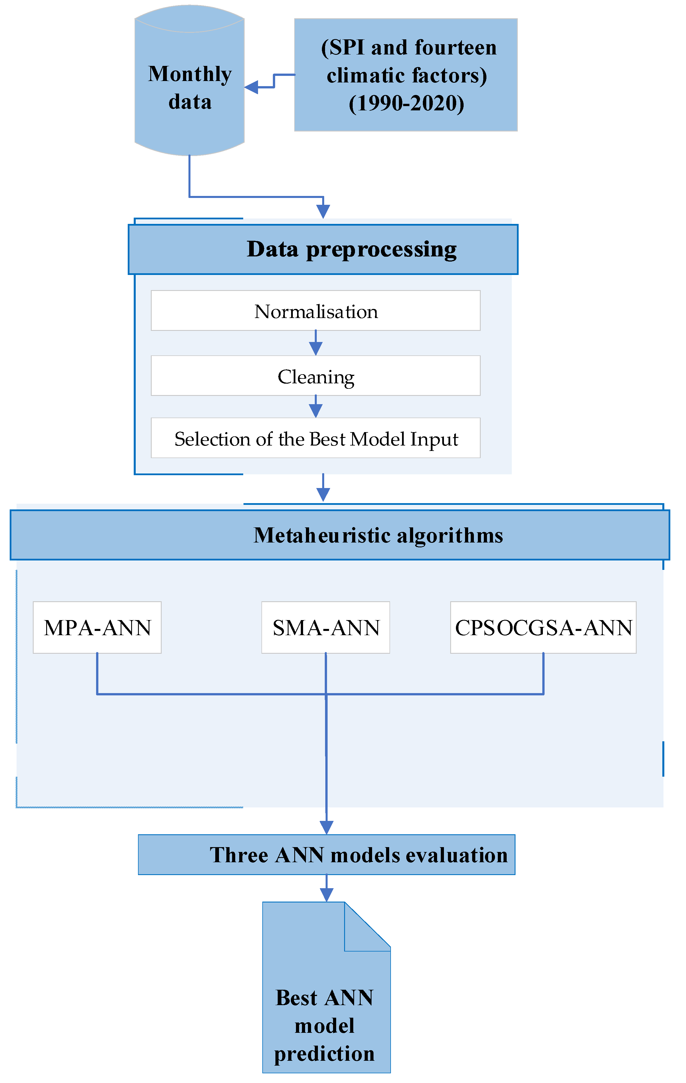
Accordingly, this study aims to evaluate a novel methodology (including data preprocessing techniques and an ANN model that integrates with different metaheuristic algorithms) to forecast the drought indices SPl 1, SPI 3, and SPI 6 for Al-Kut City, Iraq.

The primary objectives of this study are to:

• Investigate 14 climate factors over thirty years to determine to what extent climate factors drive drought indices;
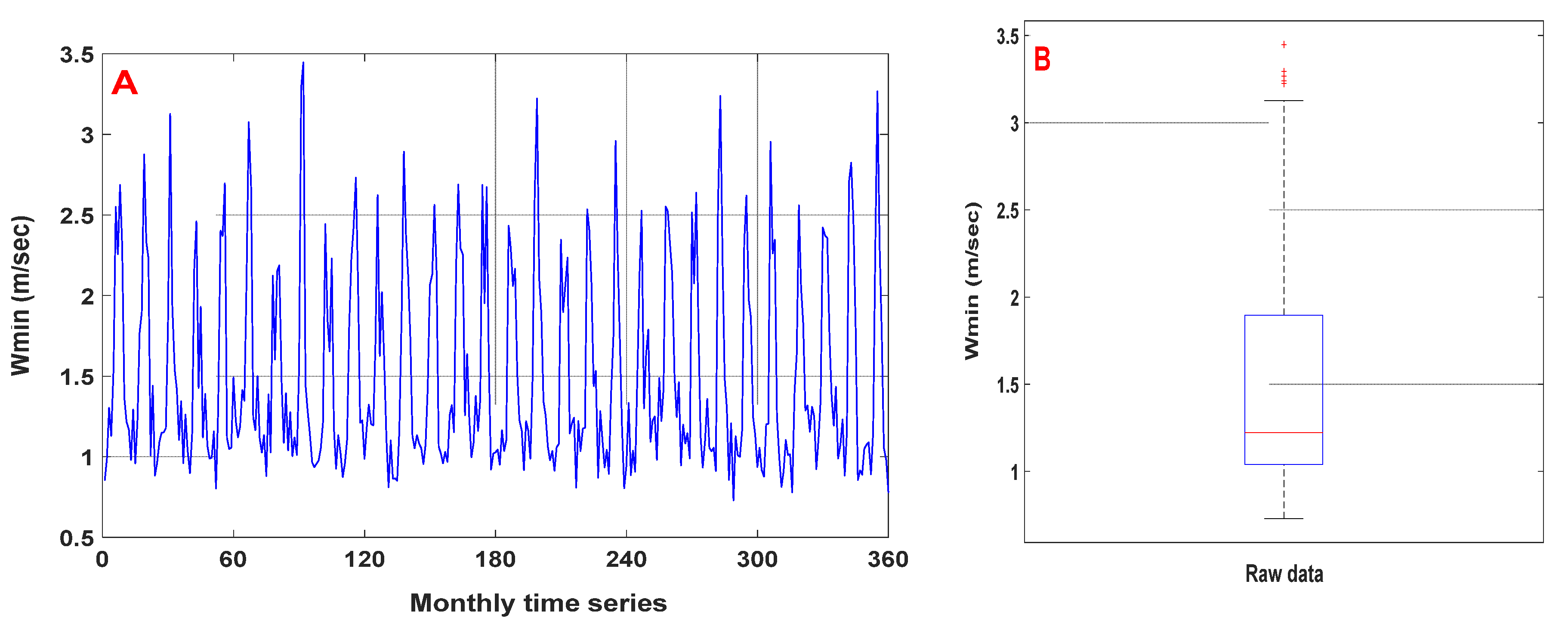
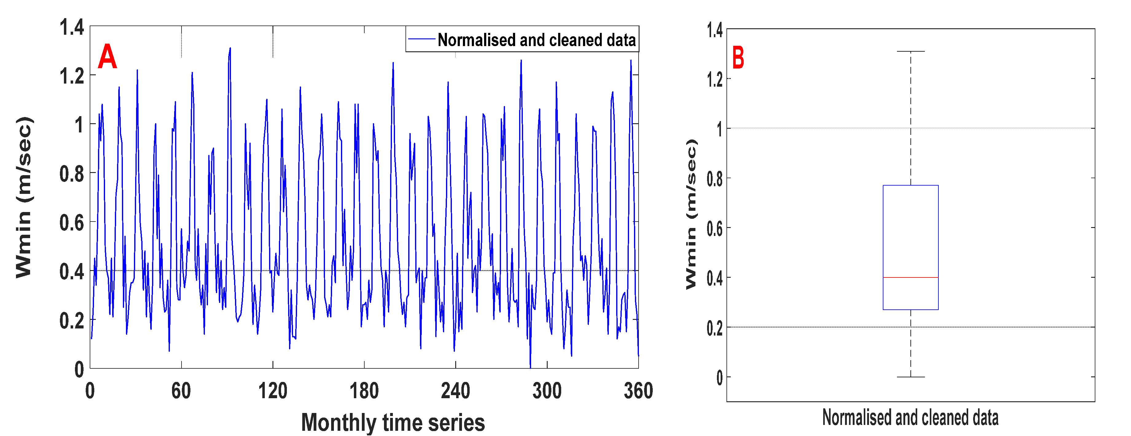
• Enhance raw data quality and identify the optimal predictor scenario;
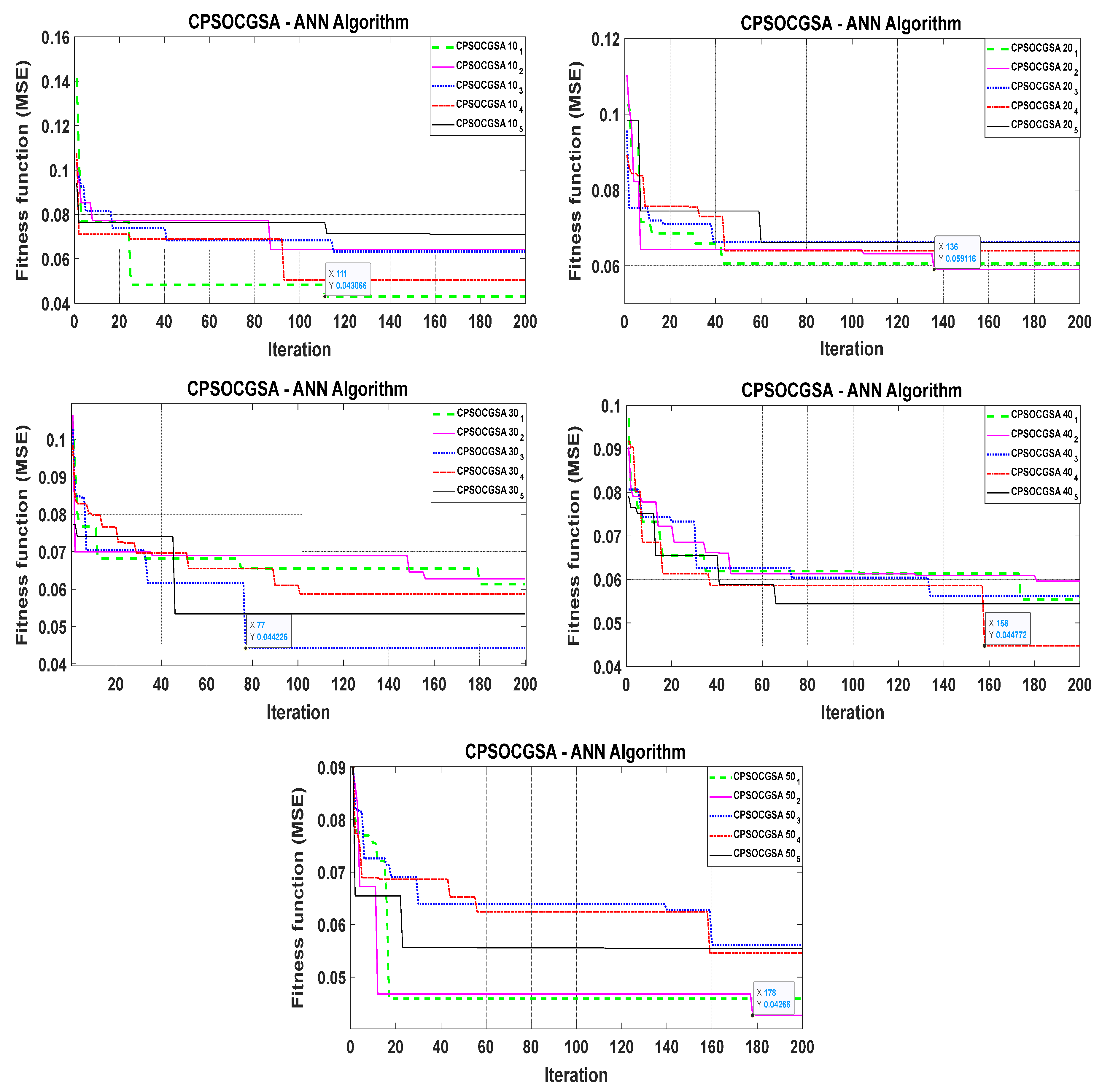
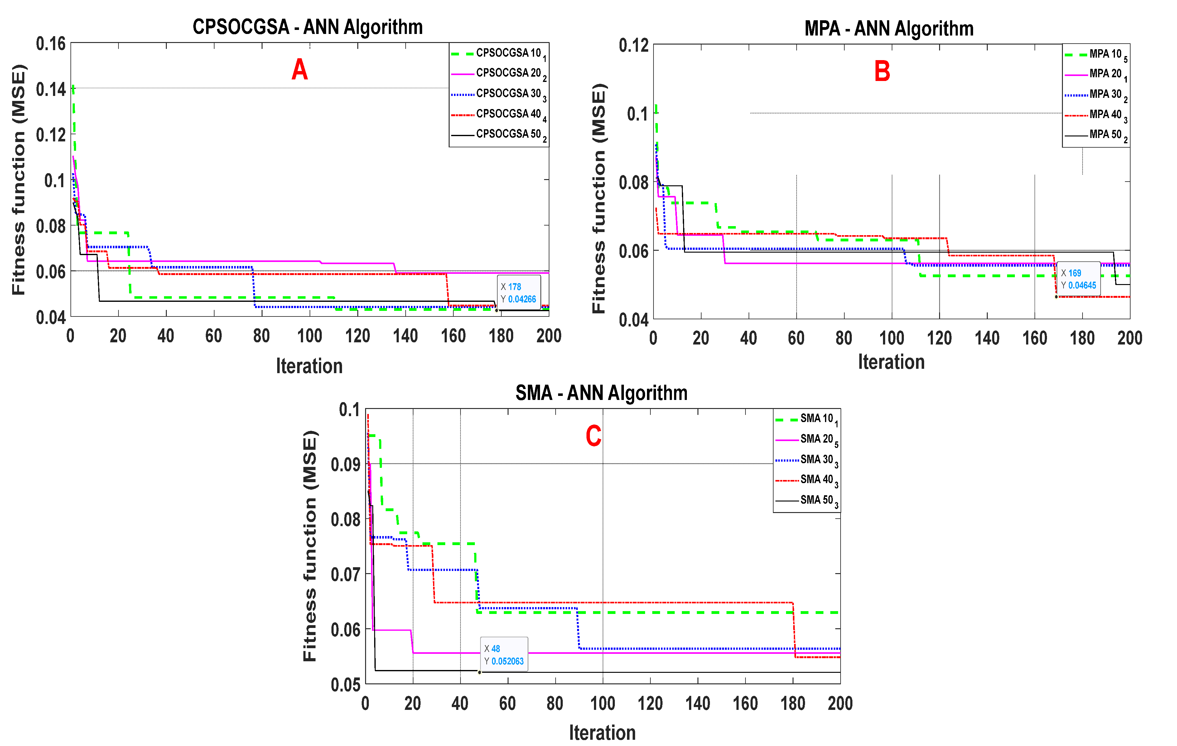
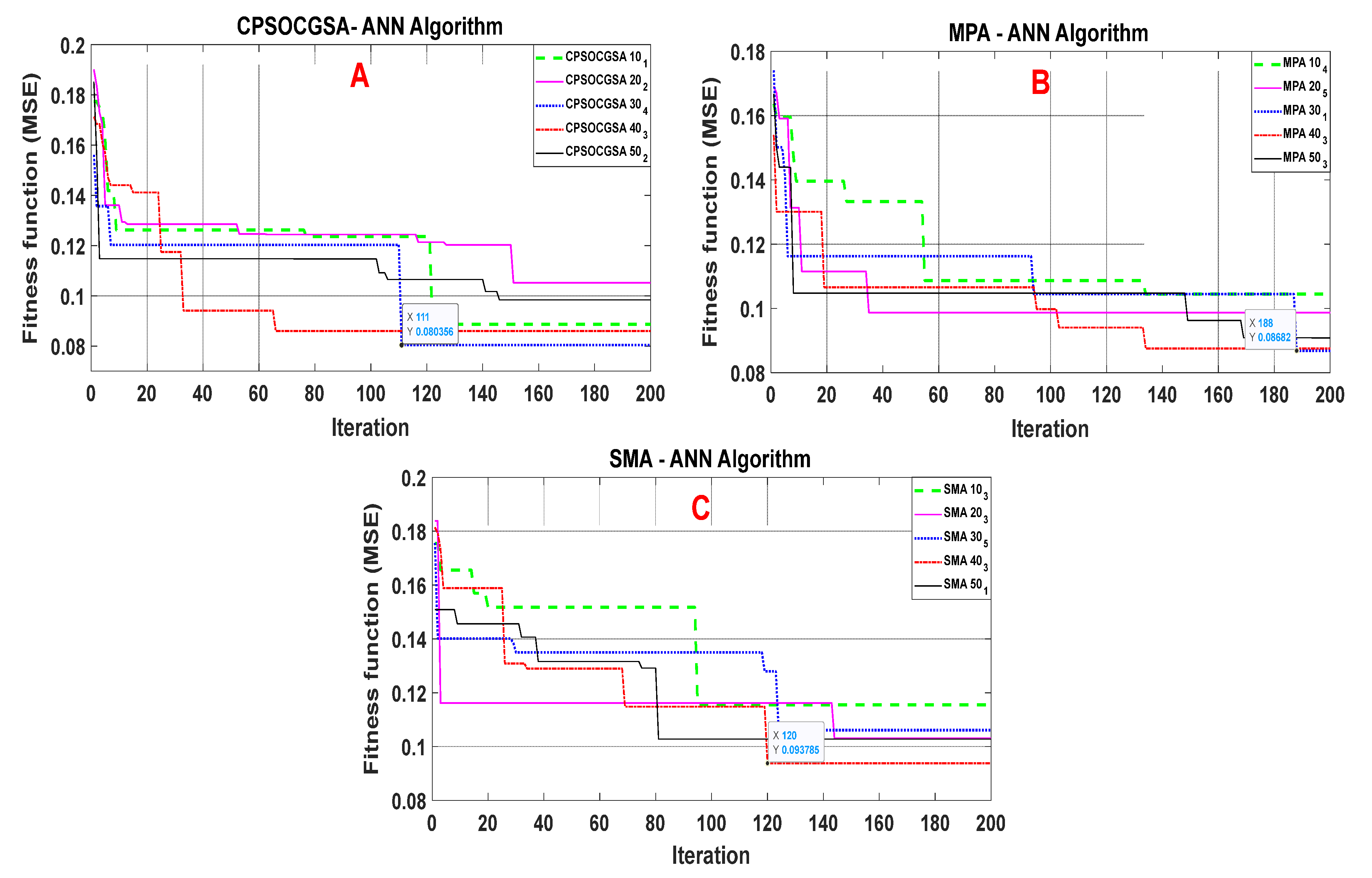
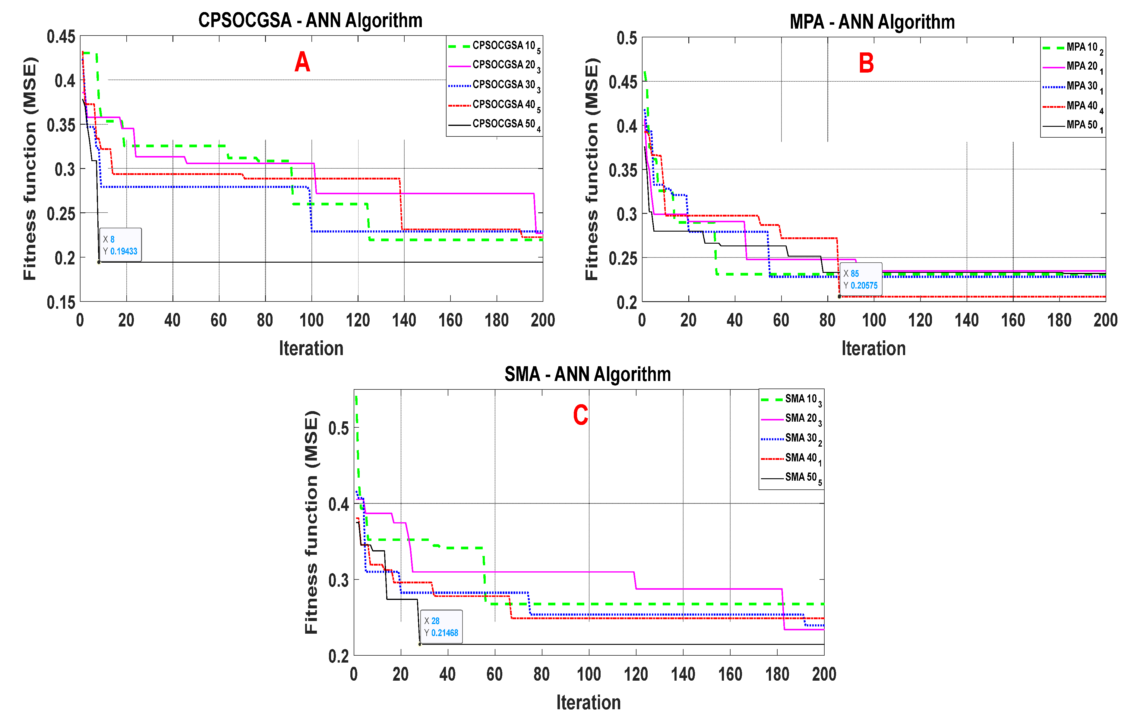
• Integrate the ANN model with the recent CPSOCGSA algorithm to choose the optimal ANN hyperparameters;
• Evaluate the CPSOCGSA-ANN technique’s performance by comparing it with the updated MPA-ANN and SMA-ANN algorithms;
• Provide a scientific view of drought to the local stakeholders because this province has the highest production and marketing of wheat in Iraq.

Based on our knowledge, this is the first time to: (a) investigate this novel methodology for forecasting drought and (b) use Al-Kut City as a study area.

The organisation of the remaining sections of this paper follows: Section 2 describes the study area and the data set employed in this study, together with the methodology utilised for constructing the prediction models. The results obtained in this study are presented in Section 3. Section 4 provides a discussion of the study’s findings. Finally, conclusions are stated in Section 5.

2. Materials and Methods

2.1. Study Area and Data Collection

Al-Kut is the Wasit region’s capital city, situated on the Tigris River in southeast Iraq. The city has an area of 17,153 square kilometres. In contrast, the built-up area of Al-Kut is around 40 square kilometres. In 2003, around 400,000 people lived in the city, and it is predicted to reach over 750,000 by 2035. Additionally, Al-Kut is considered an agricultural region characterised by wheat production [56,57]. The climate of Al-Kut City is characterised by pleasant spring and autumn seasons, cold winters, and dry and hot summers. According to the Iraqi Meteorological Department, winter begins in November and continues until March. The other seven months are considered to be summer, and the months of June, July, and August are typically the hottest of the summer [57,58].

In developing countries, the main challenge faced by many researchers is the data. In general, data from Iraqi metrological stations (1990–2020) were lost because of unusual events (i.e., embargo, terrorism, and wars). As a result, according to Ahmad, et al. [59] and Capt, et al. [60], monthly climatic factors were obtained from the National Oceanic and Atmospheric Administration (NASA) [61]. This study used the Drought Indicator Calculator (DrinC) program to calculate the SPI. DrinC program required that precipitation data be structured from October to September of the next year. It was created at the Laboratory of Reclamation Works and Water Resources Management, National Technical University of Athens, Greece [42].

The information on climatic variables was collected from 01 October 1990 to 30 September 2020. It includes minimum temperature (Tmin) (°C), mean temperature (Tmean) (°C), maximum temperature (Tmax) (°C), dew forest (DF) (°C), wet bulb temperature (Twet) (°C), rainfall (Rain) (mm/day), relative humidity (RH) (percent), surface pressure (P) (kPa), specific humidity (SH) (g/kg), maximum wind speed (Wmax) (m/s), wind speed (W) (m/s), range wind speed (Wrange) (m/s), minimum wind speed (Wmin) (m/s), and top of atmosphere (TOA) (MJ/m²/day) (Table S1 describes the statistics of climate factors). Figure 1 shows the monthly time series and boxplot for the raw minimum wind speed data. Additionally, Figures S1–S3 show the monthly time series and boxplot for rain, relative humidity, and wet bulb temperature (i.e., the other best predictors), respectively.

Table 1. The descriptive statistics of SPI time series.

Variable (Monthly)	Mean	Max.	Min.	Std. Dev.
SPI 1	0.191	2.53	−2.85	0.898
SPI 3	0.0182	2.58	−2.98	0.98
SPI 6	0.0007	2.43	−3.06	1.002

provides descriptive statistics for the drought index.

2.2. Methodology

The proposed methodology to simulate drought (i.e., SPI 1, SPI 3, and SPI 6) is based on several climatic factors, including standardised precipitation index (SPI), and its parts can be categorised into data preprocessing, constriction coefficient-based particle swarm optimisation (CCPSO), artificial neural network (ANN), and prediction accuracy criteria, as presented in Figure 2.

2.2.1. Standardised Precipitation Index (SPI)

McKee, et al. [6] introduced the SPI as a drought indicator, which the World Meteorological Organisation recognised for detecting meteorological drought characteristics [62,63]. Utilising the SPI index has several benefits: first, the SPI is easy to employ and requires only monthly rainfall data [64]. Second, the SPI can be computed on any time scale, allowing it to describe different drought types [43,65,66]. Third, since the SPI is a dimensionless index, it is possible to easily compare values across both time and space [26,67].

To calculate the SPI, the long-term rainfall record for the required period is fitted to a probability distribution, which is then converted into a normal distribution. This ensures that the mean SPI for the required period and location is zero [34]. Negative SPI values represent rainfall less than the mean, while positive values represent rainfall higher than the mean because the SPI is normalised; drier and wetter climates can be presented by using the same method [42].

Thom [68] discovered that the climatological rainfall time series follows the gamma distribution. The gamma distribution is described by the likelihood density or frequency function, as shown in Equation (1).

$$g\left(X\right)=\frac{1}{{\beta }^{\alpha }.\tau \left(\alpha \right)}{X}^{\alpha -1}.e^{-x/\beta } \mathrm{for} \mathrm{X} > 0$$

(1)

where $\tau \left(\alpha \right), \beta , \alpha , \mathrm{and} x$ represent gamma function, scale parameters, shape, and the rainfall amount, respectively. The gamma parameters β and α are computed for each station and each time scale (1, 3, 6 months, etc.). The maximum probability estimates of β and α are as follows:

$$\alpha =\frac{1}{4A}\left(1+\sqrt{1+\frac{4A}{3}} \right), where A=\ln \left(\overline{x} \right)-\frac{\sum \ln \left(x\right)}{n}$$

(2)

$$\beta =\frac{\overline{x}}{\alpha }$$

(3)

where n is the number of rainfall observations.

The resulting parameters are employed in order to calculate the cumulative probability (Equation (4)) of a recorded rainfall event for the given time scale and month for the specific area.

$$G\left(x\right)=\frac{1}{{\beta }^{\alpha }.\tau \left(\alpha \right)}.\underset{0}{\overset{x}{{\displaystyle \int }}}{x}^{\alpha -1}.e^{-\frac{x}{\beta }}.dx$$

(4)

Even though the gamma function is indeterminate for x = 0 and the rainfall distribution may include zeros, Equation (5) is employed to calculate the cumulative probability.

$$H\left(x\right)=q+\left(1-q\right).G\left(x\right)$$

(5)

where G(x) represents the gamma function’s cumulative probability and q is the probability of zero rainfall, which is calculated as follows in Equation (6):

$$q=\frac{m}{n}$$

(6)

where m is the number of zeros in a rainfall time series.

Then, the cumulative probability H(x) is converted into a standardised normal distribution at an SPI value of variance and mean equal to one and zero, respectively [42,69], as shown in Equations (7) and (8).

$$SPI=-\left(K-\frac{C_0+C_{1}K+C_2{K}^2}{1+d_{1}K+d_2{K}^2+d_3{K}^3}\right), where K=\sqrt{\ln (\frac{1}{{\left(H\left(x\right)\right)}^2})} for 0<H\left(x\right)\le 0.5$$

(7)

$$SPI=+\left(K-\frac{C_0+C_{1}K+C_2{K}^2}{1+d_{1}K+d_2{K}^2+d_3{K}^3}\right), where K=\sqrt{\ln (\frac{1}{{\left(1-H\left(x\right)\right)}^2})} for 0.5<H\left(x\right)\le 1$$

(8)

Monthly rainfall is generally not normally distributed; therefore, these values transform to fit a normal distribution that produces SPI values. The SPI is the number of standard deviations where the measured value deviates from the long-term average for a random variable with a normal distribution [70].

Table 2. Classification of drought based on SPI [72].

SPI Values	Class
>2	Extremely wet
1.5 to 1.99	Very wet
1.0 to 1.49	Moderately wet
−0.99 to 0.99	Near normal
−1 to −1.49	Moderately dry
−1.5 to −1.99	Severely dry
<−2	Extremely dry

shows a drought classification based on SPI.

Practically, droughts may be categorised depending on the time scales of rainfall. The SPI is commonly employed to define droughts based on time scales; agricultural drought can be represented by SPI 1 to SPI 6 [71]. Hence, SPI 1, SPI 3, and SPI 6 are employed due to Al-Kut being an agricultural area (i.e., a short time scale is appropriate for agriculture drought).

2.2.2. Data Preprocessing

In this study, the preprocessing of data includes three methods: normalisation, cleaning, and selection of the best model input. Details are provided below.

Normalisation

Tabachnick and Fidell [73] advised that the first choice was to employ the natural logarithm to reduce the influence of the outliers and make the distribution normal or close to normal; the second choice is to change the scores for the remaining outliers after the transformation approach. Therefore, the natural logarithm approach was applied to reduce the multicollinearity of the input variables and make the data more static [41]. This research uses the SPSS 24 statistics package.

Cleaning

Outliers and noise are leading causes for negative impact on the prediction model [73]; therefore, the box–whisker approach was employed in this research to determine outliers that exist outside of the period ± 1.5 × IQR (IQR = 3rd quartile (Q3)—1st quartile (Q1)) [74]. The SPSS 24 statistical package was used to perform the method of this approach, and the singular spectrum analysis (SSA) technique was employed to denoise the time series.

All time series contain various noise components, and the pretreatment signal is one of the most successful approaches for denoising raw time series by analysing them into multiple components [75]. Singular spectrum analysis (SSA) is commonly recognised as an adaptive noise-decreasing method employed in time series analysis [76].

Additionally, SSA has been identified as an effective preprocessing technique when combined with neural networks (or similar approaches) for time series prediction. It can be applied to both nonlinear and linear time series [9,77,78]. This strategy has been shown to be effective in a variety of fields, including industry [79], economics [80], hydrology [81], and predicting stochastic processes [82].

Selection of the Best Model Input

Selecting suitable independent variables that drive the target (dependent variable) is essential in creating the prediction model [83,84]. This study uses the tolerance technique to choose the best scenario of explanatory factors, described by Pallant [85]. The tolerance coefficient value for the selected predictors should be equal to or greater than 0.2 to avoid multicollinearity [47,85].

2.2.3. Constriction Coefficient-Based Particle Swarm Optimisation and Chaotic Gravitational Search Algorithm (CCPSOCGSA)

The present methodology is used to cover the local minima, intensification, and randomisation issues that combine the standard PSO and GSA techniques. The components of the hybrid CCPSPCGSA are explained in the following sections.

a.

Constriction Coefficient-Based Particle Swarm Optimisation (CCPSO)

The PSO is one of the well-known nature-based optimisation techniques inspired by the behaviour of birds and fish swarms. The structure of the PSO algorithm contains three key parameters. They are inertia weight, pbest, and gbest. The inertia weight has an important effect on the global exploration process. The gbest and pbest help in finding the search space region. The mathematical formulation of the PSO that describes the updating process of the location and velocity of the particles during the change in the particle values is written in Equations (9) and (10):

$$v_x^d\left(t+1\right)=w\left(t\right)v_x^d\left(t\right)+c_1{r}_{x1}\left(pbes{t}_x-x_x^d\left(t\right)\right)+c_2{r}_{x2}\left(gbest-x_x^d\left(t\right)\right)$$

(9)

$$x_x^d\left(t+1\right)=x_x^d\left(t\right)+v_x^d\left(t+1\right)$$

(10)

where are learning constants and $r_{x1}\mathrm{and} r_{x2}$ are numbers ranging from 0 to 1.

To manage the consequences of the particle movements outside the solution space and to improve the convergence during the optimisation process, a number of coefficients, called constriction coefficients, were introduced, as in Clerc and Kennedy [86]. The coefficients are described in Equations (11) and (12):

$${\phi }_1=2.05, {\phi }_2=2.05,\phi ={\phi }_1+{\phi }_2$$

(11)

$$K=2/\left(\phi -2+\sqrt{\left({\phi }^2-4\right)}\right)$$

(12)

Substituting the inertia weight by the notation K, Equation (9) can be rewritten as:

$$v_x^d\left(t+1\right)=K{v}_x^d\left(t\right)+K{\phi }_1{r}_{x1}\left(pbes{t}_x\left(t\right)-x_x^d\left(t\right)\right)+K{\phi }_2{r}_{x2}\left(gbest-x_x^d\left(t\right)\right)$$

(13)

where $K{\phi }_1=c_1$, $K{\phi }_2=c_2$.

b.

Chaotic Gravitational Search Algorithm CGSA

GSA is an optimisation technique that is inspired by Newton’s law of gravitation and motion. The GSA–based optimisation process is initialised by representing the searching agents as masses. According to Newton’s law, the gravitational force $F_{ij}$ between masses (i.e., searching agents) x and y at time t can be described as in Equation (14):

$$F_{xy}=G\left(t\right)\frac{m_{px}\left(t\right)m_{ay}\left(t\right)}{R_{xy}\left(t\right)+\in }\left(x_x^d\left(t\right)+x_y^d\left(t\right)\right)$$

(14)

where $m_{px} \mathrm{and} m_{ay}$ are the attractive and passive masses, respectively. Rxy(t) describes the Euclidian distance between the two masses at time t, while $\in$ is a small coefficient. The constant G is introduced to control the solution space for the purpose of securing a feasible region. The constant G can be described as in Equation (15):

$$G\left(t\right)=G\left(t_o\right)e^{\left(-\alpha \frac{CI}{MI}\right)}$$

(15)

where $G\left(t\right) \mathrm{and} G\left(t_o\right)$ are the final and initial values of G, $\alpha$ is a small constant, $CI$ is the current iteration, and $MI$ is the maximum number of iterations.

The behaviour of G over time is proposed by Rather and Bala [87] using a chaotic normalisation process. Thus, the final description of the gravitational constant can be formulated as in Equation (16):

$$G^c\left(t\right)=C_i^{norm}\left(t\right)+G\left(t_o\right)e^{\left(-\alpha \frac{CI}{MI}\right)}$$

(16)

The total force exerted by the masses (i.e., searching agents) can be calculated as in Equation (17):

$$F_x^d\left(t\right)={\displaystyle \sum }_{y=1, y\ne x}^m{\gamma }_y{F}_{xy}$$

(17)

where $\gamma$ value ranges from 0 to 1.

The position and velocity can be represented according to Equations (18) and (19):

$$v_x^d\left(t+1\right)={\gamma }_y{v}_x^d\left(t\right)+a_x^d\left(t\right)$$

(18)

$$x_x^d\left(t+1\right)=x_x^d\left(t\right)+v_x^d\left(t+1\right)$$

(19)

where $a_x^d\left(t\right)$ is the acceleration of the mass.

c.

Combination of CCPSO and CGSA

The combination of CPSO and CGSA leads to combining the diversification and convergence properties of the two techniques. The combination results are described in Equation (20):

$$\begin{gathered} v_x^d\left(t+1\right)=\left(2/\left(\phi -2+\sqrt{{\phi }^2-4}\right)\right)v_x^d\left(t\right)+K{\phi }_1{r}_{x1}\left(a_x^d\left(t\right)-x_x^d\left(t\right)\right) \\ +K{\phi }_2{r}_{x2}\left(gbest-x_x^d\left(t\right)\right) \end{gathered}$$

(20)

The location of the particles is given by Equation (21):

$$x_x^d\left(t+1\right)=x_x^d\left(t\right)+v_x^d\left(t+1\right)$$

(21)

2.2.4. Artificial Neural Network (ANN)

ANN is a computational system for information processing inspired by the human brain [88,89]. The benefits of employing ANNs follow: small data needs; capacity to construct models when the link between inputs and outputs is not completely understood; quick execution time; and, finally, ability to predict nonstationary and nonlinear time series data in the fields of hydrology and water resources [2,32,90]. These properties make ANNs appropriate for drought prediction [29]. This study implements the multilayer perceptron (MLP) to simulate the standardised precipitation index. MLP applied feed-forward backpropagation (FFBB) that used the Levenberg–Marquardt learning algorithm (LM) for training the ANN model due to its speed, efficiency, and low error rate, as shown by Payal, et al. [91]. The MLP structure consists of four layers: the first is the input layer that has climatic variables (Rain, RH, Twet, and Wmin); followed by two hidden layers that contain the tansigmoidal activation function to manage complex nonlinearity and the output layer that includes SPI. Moreover, the trial-and-error approach does not always provide the optimal solution and considers time consumption. Therefore, metaheuristic algorithms were integrated with ANN to select the optimal value of the learning rate and the best number of neurons for hidden layers to obtain the best input/output mapping and avoid overfitting or underfitting the model [41]. The model was also applied using the Neural Network Toolbox for MATLAB. Furthermore, following Soh, et al. [23] and Zhang, et al. [3], the data were divided into three groups: training (70%, from 1990 to 2010); testing (15%, from 2011 to 2015); and validation (15%, from 2016 to 2020) to build and assess the forecasting model.

2.3. Prediction Accuracy Criteria

This research evaluated the performance of models in SPI prediction by employing three statistical criteria. The applied metrics are mean absolute error (MAE), root-mean-squared error (RMSE), and determination coefficient (R²). The following formulae can be used to calculate them [92,93]:

$$\mathrm{MAE}=\frac{{\sum }_{i=1}^N\left|O_i-F_i\right|}{N}$$

(22)

$$\mathrm{RMSE}=\sqrt{\frac{{\sum }_{i=1}^N{\left(O_i-F_i\right)}^2}{N}}$$

(23)

$$R^2{}^{ }={\left[\frac{{\sum }_{i=1}^N\left(O_i-{\overline{O}}_i\right)\left(F_i-F_i\right)}{\sqrt{\sum {\left(O_i-{\overline{O}}_i\right)}^2\sum {\left(F_i-{\overline{F}}_i\right)}^2}}\right]}^2$$

(24)

where $O_i$ represents observed $\mathrm{SPI}$, $F_i$ is the predicted SPI, N is the sample size, $\overline{F_i}$ is the mean of predicted SPI, and $\overline{O_i}$ is the mean of observed SPI.

In addition, this research employed Taylor diagrams to compare the modelling results, which provide pattern statistics to prepare a visual comprehension of performance by displaying various points on a polar plot for two or more sets of modelling outcomes [94]. Additionally, three tests were used to assess the residual analysis: the Kolmogorov–Smirnov, Shapiro–Wilk, and residual analysis plot.

3. Results

3.1. Input Data Analysis

The climatic factors (independent variables) data were normalised, as mentioned in Section 2.2.2. Additionally, the time series for dependent variables (SPI 1, SPI 3, and SPI 6) and climatic factors were cleaned according to Section 2.2.2. Figure 3 shows the normalised and cleaned data for wind speed minimum. The time series variance has decreased in Figure 3A compared to Figure 1A. Additionally, Figure 3B shows the time series cleaned from outliers that appear in Figure 1B.

Then, the pretreatment signal technique (SSA) was utilised to obtain the time series data for SPI 1, SPI 3, SPI 6, and all climatic variables without noise. Figure 4 shows the original time series (cleaned data) for SPI 6 (first line), the new time series (second line) and two noise signals (third and fourth lines).

In the last step of data preprocessing methods, a tolerance technique was employed to choose the best scenario of model input (climatic factors) to simulate the SPI precisely and avoid multicollinearity by removing superfluous variables. After applying various scenarios, the best scenario was chosen based on tolerance coefficients that were equal to or greater than 0.2 for all nominated predictors. This strategy was used for SPI 1, SPI 3, and SPI 6 models, as presented in

Table 3. Statistics of collinearity for the chosen best input variables.

Target	Climatic Variables	Tolerance Value
SPI 1	Rain	0.292
	RH	0.240
	Twet	0.577
	Wmin	0.678
SPI 3	Rain	0.292
	RH	0.241
	Twet	0.578
	Wmin	0.682
SPI 6	Rain	0.291
	RH	0.242
	Twet	0.579
	Wmin	0.686

. It can be seen that four climatic factors, Rain, RH, Twet, and Wmin, were chosen to be the best predictors’ scenarios for the three SPI models.

The impact of data preprocessing on the correlation coefficient (R) between input and output data was assessed, and it found that the data preprocessing enhanced the correlation coefficient values between standardised precipitation indices (SPI 1, SPI 3, and SPI 6) and climatic variables; for example, the correlation coefficient for rain increased from 0.507 to 0.945, 0.446 to 0.936, and 0.373 to 0.866 for SPI 1, SPI 3, and SPI 6, respectively. Accordingly, the preprocessing data methods improved the data quality for both dependent and independent time series.

3.2. Application of the Hybrid Heuristic Algorithms—ANN Approach

The ANN approach requires combination with a metaheuristic algorithm to find the optimal learning rate (Lr) and the number of neurons in both hidden layers (N1 and N2). A MATLAB toolbox was employed to run the CPSOCGSA-ANN, MPA-ANN, and SMA-ANN algorithms to determine the best hyperparameters for the ANN model. For each algorithm, this research applied the swarm size (10, 20, 30, 40, and 50 swarms) five times for each swarm with 200 iterations to gain a minimum fitness function (MSE). Figure 5 shows an example of the CPSOCGSA-ANN algorithm performance and reveals the best fitness function for each swarm for SPI 1.

Figure 6A presents the best swarm size 50_{_2} of the CPSOCGSA-ANN algorithm for SPI 1 that provides less MSE = 0.04266 after 178 iterations. Additionally, Figure 6B shows the swarm size 40_{_3} offers the minimum MSE = 0.04645 after 169 iterations for the MPA-ANN algorithm. Additionally, the swarm size 50_{_3} gives less MSE = 0.052063 after 48 iterations for the SMA-ANN algorithm, as presented in Figure 6C.

Figure 7A displays that the 30_{_4} swarm size gives the best solution for the CPSOCGSA-ANN algorithm (MSE = 0.080356, after 111 iterations) for SPI 3, while in Figure 7B, the 30_{_1} swarm size provides the best solution for the MPA-ANN algorithm (MSE = 0.08682, after 188 iterations). Figure 7C presents the swarm size 40_{_3} and offers the optimal solution for the SMA-ANN algorithm (MSE = 0.093785, after 120 iterations).

Figure 8A shows that the swarm size 50_{_4} offers the best answer with less fitness function (MSE = 0.19433 after eight iterations) for the CPSOCGSA-ANN algorithm. While in Figure 8B, the hybrid MPA-ANN algorithm reveals that the swarm size 40_{_4} provides the optimal answer with less fitness function (MSE = 0.20575 after 85 iterations). Figure 8C shows that the swarm size 50_{_5} gives the best solution for the hybrid SMA-ANN algorithm based on MSE equal to 0.21468 after 28 iterations for SPI 6. Based on the results of hybrid models for each SPI model, each best swarm for each hybrid model offers optimal hyperparameters for the ANN model. Accordingly,

Table 4. ANN parameters are based on algorithms for SPI 1, SPI 3, and SPI 6.

Model	Parameter	CPSOCGSA	MPA	SMA
SPI 1	N1	3	5	7
	N2	7	5	13
	Lr	0.3686	0.0010	0.4192
SPI 3	N1	4	10	3
	N2	5	1	14
	Lr	0.5841	0.1115	0.6413
SPI 6	N1	5	9	3
	N2	3	1	4
	Lr	0.2747	0.0013	0.2570

N1 and N2 represent the number of neurons in hidden layers one and two, respectively. LR is the learning rate of the ANN.

shows the ANN hyperparameters for the best swarm size for each algorithm and SPI model.

3.3. Evaluating and Comparing the Performance of the Algorithms with ANN

Following the procedure of Adnan, et al. [43] and Aghelpour, et al. [62], three ANN models were constructed using the hyperparameters (Table 4). Each ANN model was run numerous times to discover the best structure of the neural network (weights) capable of accurately forecasting SPI 1. The performance of the models was evaluated using three statistical criteria (see Section 2.3). This strategy was performed for SPI 3 and SPI 6 as well.

Table 5. Performance assessment criteria for CPSOCGSA, MPA, and SMA in the validation stage.

Target	Model	R2	MAE	RMSE
SPI 1	CPSOCGSA-ANN	0.93	0.0635	0.0791
	MPA-ANN	0.86	0.0840	0.0976
	SMA-ANN	0.78	0.0961	0.1127
SPI 3	CPSOCGSA-ANN	0.93	0.1020	0.1270
	MPA-ANN	0.91	0.1172	0.1344
	SMA-ANN	0.86	0.1220	0.1676
SPI 6	CPSOCGSA-ANN	0.88	0.2004	0.2334
	MPA-ANN	0.86	0.2186	0.2589
	SMA-ANN	0.78	0.2618	0.3001

shows the statistical indicators (R², MAE, and RMSE) for each hybrid model for the SPI 1, SPI 3, and SPI 6 prediction models. According to Dawson, et al. [95], the CPSOCGSA-ANN and MPA-ANN models showed good forecasting accuracy for SPI 1, SPI 3, and SPI 6, and the SMA-ANN model for SPI 3 that yielded R² greater than 0.85. The results also demonstrated that the CPSOCGSA-ANN model is preferable to MPA-ANN and SMA-ANN for SPI models, and that the SMA-ANN model was the worst.

The Taylor diagram was employed to examine the drought forecasting results for further assessment. This diagram shows a graphical view of the agreement between predicted and measured patterns, considering the blue azimuthal line, a green contour line, and a black arc representing the value of the correlation coefficient (R), the root-mean-square difference (RMSD), and standard deviation (SD), respectively. Figure 9 shows the Taylor diagram for the CPSOCGSA-ANN, MPA-ANN, and SMA-ANN forecasting models for SPI 1, SPI 3, and SPI 6.

For SPI 1, performance predictions for all the models fall within the correlation coefficient range 0.88 to 0.97. In addition, the CPSOCGSA-ANN and MPA-ANN are located between the contour lines (0.05 and 0.1) according to RMSD, while the SMA-ANN is situated beyond the 0.1 contour line.

For SPI 3, the Taylor diagram shows that the correlation coefficient of forecasting models is located between 0.92 and 0.97. Additionally, all models were found between contour lines 0.1 and 0.2 according to RMSD.

For SPI 6, the performance of the simulation models is located within the correlation range 0.88 to 0.94. According to RMSD, all models are found between the same range of contour lines (0.2 and 0.4).

In all cases, the CPSOCGSA-ANN is nearest to the observed drought (reference), followed by MPA-ANN, and lastly, SMA-ANN. Therefore, CPSOCGSA-ANN is superior to the MPA-ANN and SMA-ANN, as shown in Figure 9. Additionally, for the CPSOCGSA-ANN technique, SPI 1 performs better than SPI 3 and SPI 6 models, and the accuracy tends to decline steadily from SPI 1 to SPI 6.

A graphical test was employed to confirm the capability of the hybrid models to generalise SPI time series (i.e., SPI 1, SPI 3, and SPI 6) in the validation stage. Figure 10 shows the measured SPI data and predicted SPI data from CPSOCGSA-ANN, MPA-ANN, and SMA-ANN. It can be noticed that the forecasted data from CPSOCGSA-ANN follows the trend and periodicity of the measured data, and it is the closest to the measured data from MPA-ANN and SMA-ANN according to the scale of error. Several slight deviations in the predicted time series may have resulted from the effect of climatic factors’ fluctuations.

The results of this study affirmed that the CPSOCGSA-ANN outperforms the MPA-ANN and SMA-ANN models. For more examinations of the CPSOCGSA-ANN model, Kolmogorov–Smirnov (K-S) and Shapiro–Wilk (S-W) tests were employed to check the normality of the residual data, as shown in

Table 6. Tests of normality.

Target	Kolmogorov–Smirnova (K–S)	Shapiro–Wilk (S–W)
SPI 1	0.200	0.224
SPI 3	0.200	0.545
SPI 6	0.200	0.340

. The finding reveals that the residuals follow a normal distribution because the outcomes of the K–S and S–W tests showed a p-value > 0.05, according to Valentini, et al. [96]. In addition, Figure 11 shows the normal distribution of the residual data for SPI 1, SPI 3, and SPI 6.

Based on the above results of statistical and graphical tests and residual analysis, it is possible to conclude that:

(1)

These results show the ability of SSA and tolerance strategies to enhance the quality of raw data and choose the optimal predictors scenario without transgressing the multicollinearity supposition.

(2)

Rain, RH, Twet, and Wmin emerged as reliable predictors of SPI 1, SPI 3, and SPI 6.

(3)

The CPSOCGSA-ANN method is a reliable model that can accurately predict the short-term drought index, outperforming the MPA-ANN and SMA-ANN models.

(4)

The proposed methodology (i.e., hybridisation of preprocessing-based with parameter optimisation-based hybrid models) accurately predicted monthly drought according to various statistical criteria.

(5)

The findings reveal a strong relationship between drought and climatic factors.

This study focuses on the proposed methodology for predicting drought for cities that suffer from variability in socioeconomic factors and climate, such as Al-Kut city. As a result, policymakers and stakeholders can find this procedure helpful in making intelligent decisions and developing effective plans for irrigation system operation.

4. Discussion

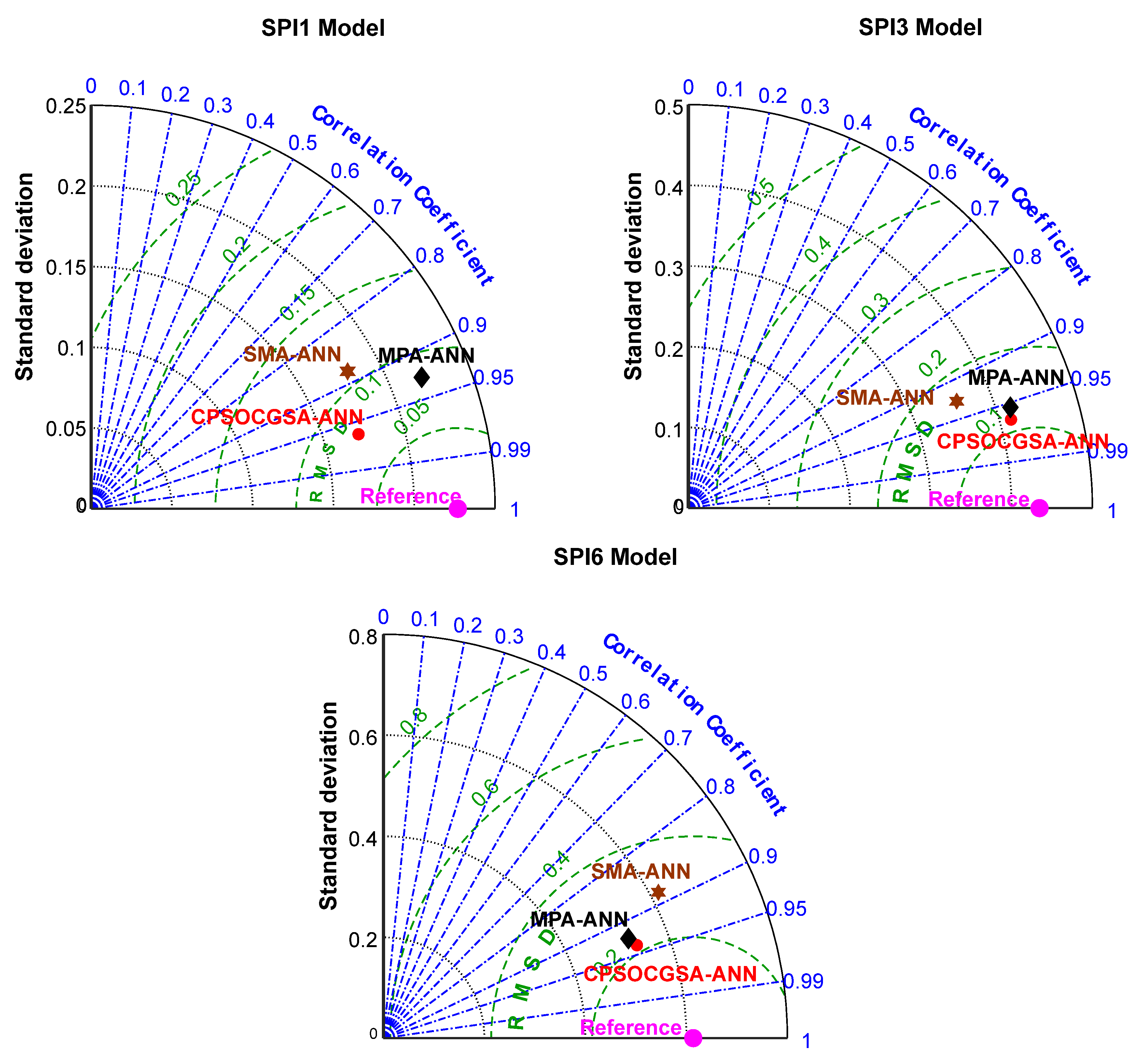
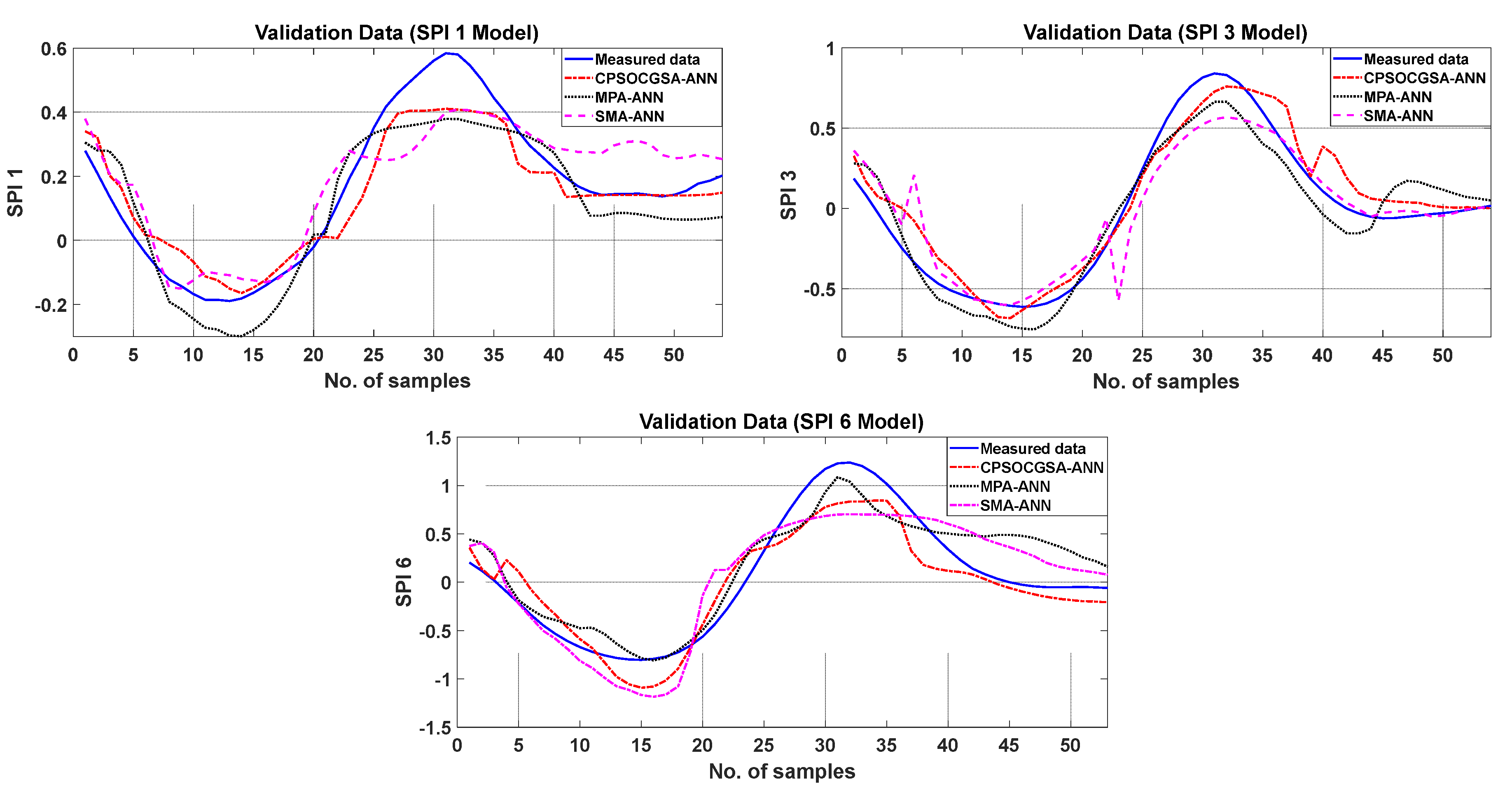
Droughts may have devastating consequences on socioeconomic and environmental conditions, but the agricultural sector is the most severely impacted by drought. Al-Kut is considered an agricultural area that is characterised by wheat production. Therefore, drought prediction is essential for mitigating the effects of droughts in the region. Based on our knowledge, no article has been published to predict droughts in the study area. As a result, the present study forecasts the standardised precipitation index using various machine learning techniques (CPSOCGSA-ANN, ANN-MPA, and ANN-SMA) with different time scales (SPI 1, SPI 3, and SPI 6).

During the validation stage, the models with lowest RMSE, MAE, and greatest R² are considered the best for predicting drought. This study reveals that predictions of SPI by using CPSOCGSA-ANN were the most accurate across all time scales (SPI 1, SPI 3, and SPI 6). This model can help the local authorities (managers and decision-makers) make intelligent decisions and improve effective irrigation system operation plans.

The artificial neural network (ANN) result was compared with support vector regression (SVR) to predict temporal drought occurrences in Australia. The findings showed that ANN outperformed SVR, with the former having the higher R² value of 0.86 compared to 0.75 for the latter [33]. Despite the high ability of ANN in forecasting hydroclimate parameters (e.g., rainfall), this technique may show limitations in dealing with hydrological time series that are often nonstationary and cover a broad range of scales. As a result, data preprocessing may be a significant stage in overcoming defects and similar issues [97]. Khan, et al. [98] employed ANN and the hybrid ANN with wavelet (W-ANN) for predicting drought in Malaysia. The results show that the wavelet method achieved higher correlation coefficients (i.e., W-ANN outperforms the single ANN). The least-square support vector machine (LSSVM) and LSSVM-singular spectrum analysis (SSA-LSSVM) were used to predict the standardised precipitation index (SPI) for Taiwan. Prediction accuracy was higher for SSA-LSSVM than for LSSVM [4]. Başakın, et al. [28] evaluated the adaptive neurofuzzy inference system (ANFIS) and ANFIS with empirical mode decomposition (ANFIS-EMD) to predict drought. The statistical indicators MSE and NSE reveal that the combined EMD-ANFIS model is better than the ANFIS model when employed singularly. Bioinspired optimisation algorithms have been effectively utilised to improve model abilities by identifying the optimal hyperparameters of ML models [5,99]. Banadkooki, et al. [5] utilised ANN models with three metaheuristic optimisation algorithms, namely particle swarm optimisation (PSO), the salp swarm algorithm (SSA), and the genetic algorithm (GA), to predict drought in the Yazd plain, Iran. The result reveals that SSA-ANN outperforms PSO-ANN and GA-ANN. Nabipour, et al. [25] proposed a combined model of artificial neural networks (ANN) with different metaheuristic algorithms, including the salp swarm algorithm (SSA), grasshopper optimization algorithm (GOA), particle swarm optimization (PSO), and biogeography-based optimisation (BBO) for predicting short-term drought in Iran. According to the results, the combined model outperformed the single ANN.

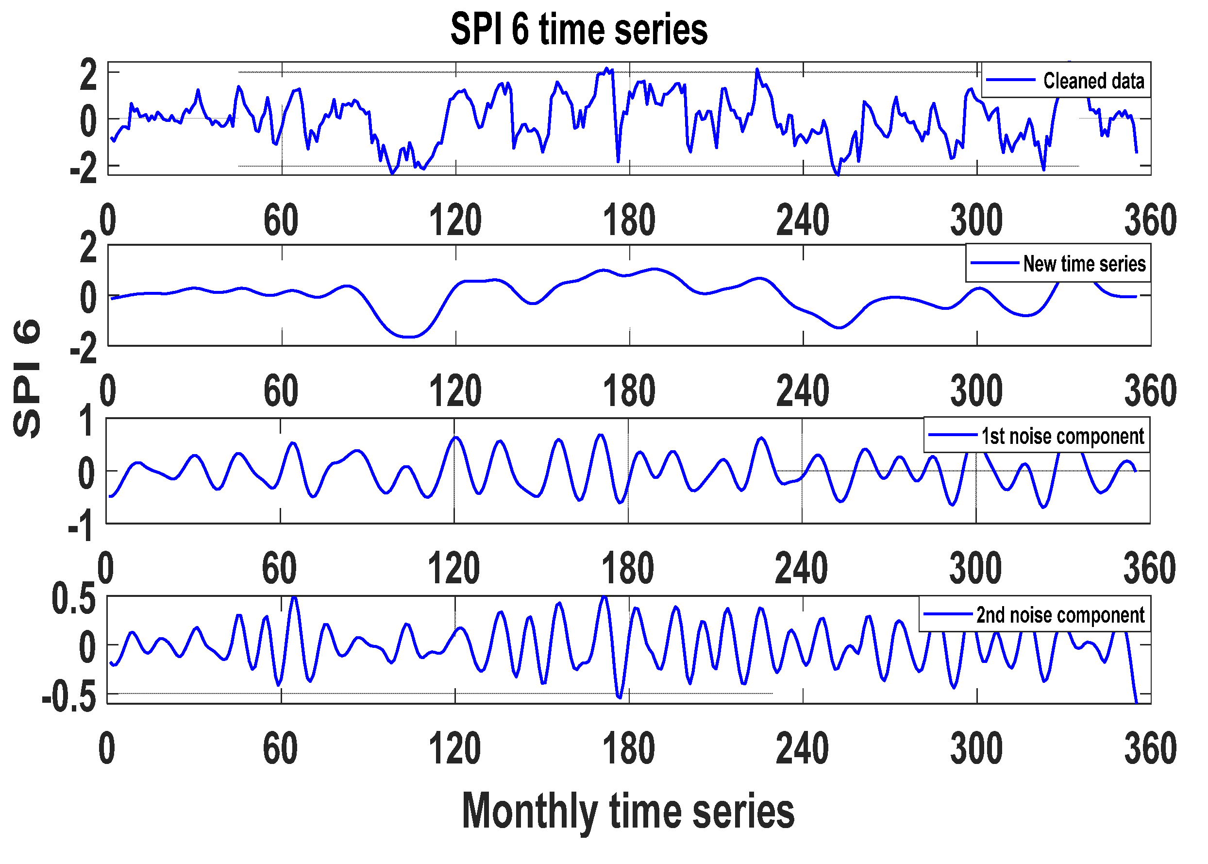
The literature described above indicates that the hybridised version of the machine learning techniques is better than standalone models in forecasting drought. The present study shows that data preprocessing (i.e., normalisation, cleaning, and best model input) increased the correlation coefficient values between standardised precipitation indices (SPI 1, SPI 3, and SPI 6) and climatic variables (Section 3.1). Moreover, this study showed that the hybrid ML model, specifically ANN-CPSOCGSA, was more accurate in drought prediction with different time scales (SPI 1, SPI 3, and SPI 6). Furthermore, the results of this study indicate that the drought simulation model may be installed as an early warning system in the Al-Kut region to mitigate the effects of drought.

5. Conclusions

The accuracy of future drought forecasting is critical for risk management, agriculture irrigation, and drought preparation. Climate variables play a significant role in drought forecasting. Drought is driven effectively by rainfall, temperature, wind speed, and relative humidity. Therefore, the effects of climate variables cannot be neglected in drought forecasting. This study suggested a novel hybrid methodology to simulate drought (SPI 1, SPI 3, and SPI 6) based on climatic factors over 30 years in Al-Kut City, Iraq. The methodology includes data preprocessing techniques and an ANN model integrated with the recent CPSOCGSA algorithm. Additionally, the MPA and SMA algorithms were applied to assess and validate the performance of the CPSOCGSA algorithm. The results reveal that the data preprocessing techniques (i.e., SSA and tolerance) effectively denoise time series and remove the redundant predictors leading to improving the data quality and selecting the best predictors scenario. The performance of CPSOCGSA-ANN outperforms both the MPA-ANN and SMA-ANN algorithms based on different statistical criteria (i.e., R², MAE, and RMSE). The best models predicted SPI 1 with R² = 0.93, MAE = 0.0635, and RMSE = 0.0791, SPI 3 with R² = 0.93, MAE = 0.1020, and RMSE = 0.1270, and SPI 6 with R² = 0.88, MAE = 0.2004, and RMSE = 0.2334. Additionally, the results indicate that the proposed model can be successfully applied in predicting drought for regions that suffer from variability in socioeconomic and climate variables. These findings can provide beneficial information to the local authorities (i.e., managers and decision-makers), helping the irrigation sector company to manage the irrigation system better, leading to improved service and management of resources in Al-Kut city. For future research, this study offers a framework for exploring and investigating innovative hybrid models that combine preprocessing and parameter optimisation. Further research using the same hybrid techniques to forecast different drought indices is needed for various regions.

References

1. Xu, D.; Zhang, Q.; Ding, Y.; Zhang, D. Application of a hybrid ARIMA-LSTM model based on the SPEI for drought forecasting. Environ. Sci. Pollut. Res. Int. 2022, 29, 4128–4144. [Google Scholar] [CrossRef]
2. Belayneh, A.; Adamowski, J.; Khalil, B.; Ozga-Zielinski, B. Long-term SPI drought forecasting in the Awash River Basin in Ethiopia using wavelet neural network and wavelet support vector regression models. J. Hydrol. 2014, 508, 418–429. [Google Scholar] [CrossRef]
3. Zhang, Y.; Li, W.; Chen, Q.; Pu, X.; Xiang, L. Multi-models for SPI drought forecasting in the north of Haihe River Basin, China. Stoch. Environ. Res. Risk Assess. 2017, 31, 2471–2481. [Google Scholar] [CrossRef]
4. Pham, Q.B.; Yang, T.-C.; Kuo, C.-M.; Tseng, H.-W.; Yu, P.-S. Coupling Singular Spectrum Analysis with Least Square Support Vector Machine to Improve Accuracy of SPI Drought Forecasting. Water Resour. Manag. 2021, 35, 847–868. [Google Scholar] [CrossRef]
5. Banadkooki, F.B.; Singh, V.P.; Ehteram, M. Multi-timescale drought prediction using new hybrid artificial neural network models. Nat. Hazards 2021, 106, 2461–2478. [Google Scholar] [CrossRef]
6. McKee, T.B.; Doesken, N.J.; Kleist, J. The relationship of drought frequency and duration to time scales. In Proceedings of the 8th Conference on Applied Climatology, Anaheim, CA, USA, 17–22 January 1993. [Google Scholar]
7. Anshuka, A.; van Ogtrop, F.F.; Willem Vervoort, R. Drought forecasting through statistical models using standardised precipitation index: A systematic review and meta-regression analysis. Nat. Hazards 2019, 97, 955–977. [Google Scholar] [CrossRef]
8. Gumus, V.; Algin, H.M. Meteorological and hydrological drought analysis of the Seyhan−Ceyhan River Basins, Turkey. Meteorol. Appl. 2017, 24, 62–73. [Google Scholar] [CrossRef]
9. Zubaidi, S.L.; Dooley, J.; Alkhaddar, R.M.; Abdellatif, M.; Al-Bugharbee, H.; Ortega-Martorell, S. A Novel approach for predicting monthly water demand by combining singular spectrum analysis with neural networks. J. Hydrol. 2018, 561, 136–145. [Google Scholar] [CrossRef]
10. Sa’adi, Z.; Shahid, S.; Ismail, T.; Chung, E.-S.; Wang, X.-J. Distributional changes in rainfall and river flow in Sarawak, Malaysia. Asia Pac. J. Atmos. Sci. 2017, 53, 489–500. [Google Scholar] [CrossRef]
11. Salman, S.A.; Shahid, S.; Ismail, T.; Ahmed, K.; Chung, E.-S.; Wang, X.-J. Characteristics of Annual and Seasonal Trends of Rainfall and Temperature in Iraq. Asia Pac. J. Atmos. Sci. 2019, 55, 429–438. [Google Scholar] [CrossRef]
12. Salman, S.A.; Shahid, S.; Ismail, T.; Chung, E.-S.; Al-Abadi, A.M. Long-term trends in daily temperature extremes in Iraq. Atmos. Res. 2017, 198, 97–107. [Google Scholar] [CrossRef]
13. Nashwan, M.S.; Shahid, S.; Abd Rahim, N. Unidirectional trends in annual and seasonal climate and extremes in Egypt. Theor. Appl. Climatol. 2018, 136, 457–473. [Google Scholar] [CrossRef]
14. Ethaib, S.; Zubaidi, S.L.; Al-Ansari, N.; Fegade, S.L. Evaluation water scarcity based on GIS estimation and climate-change effects: A case study of Thi-Qar Governorate, Iraq. Cogent Eng. 2022, 9, 2075301. [Google Scholar] [CrossRef]
15. Aljanabi, A.A.; Mays, L.W.; Fox, P. A Reclaimed Wastewater Allocation Optimization Model for Agricultural Irrigation. Environ. Nat. Resour. Res. 2018, 8, 55. [Google Scholar] [CrossRef]
16. Salman, S.A.; Shahid, S.; Ismail, T.; Rahman, N.b.A.; Wang, X.; Chung, E.-S. Unidirectional trends in daily rainfall extremes of Iraq. Theor. Appl. Climatol. 2017, 134, 1165–1177. [Google Scholar] [CrossRef]
17. Osman, Y.; Abdellatif, M.; Al-Ansari, N.; Knutsson, S.; Jawad, S. Climate change and future precipitation in an arid environment of the middle east: Case study of Iraq. J. Environ. Hydrol. 2017, 25, 3. [Google Scholar]
18. Bandyopadhyay, N.; Bhuiyan, C.; Saha, A.K. Drought mitigation: Critical analysis and proposal for a new drought policy with special reference to Gujarat (India). Prog. Disaster Sci. 2020, 5, 100049. [Google Scholar] [CrossRef]
19. Adnan, S.; Ullah, K.; Shuanglin, L.; Gao, S.; Khan, A.H.; Mahmood, R. Comparison of various drought indices to monitor drought status in Pakistan. Clim. Dyn. 2017, 51, 1885–1899. [Google Scholar] [CrossRef]
20. Adede, C.; Oboko, R.; Wagacha, P.W.; Atzberger, C. A Mixed Model Approach to Vegetation Condition Prediction Using Artificial Neural Networks (ANN): Case of Kenya’s Operational Drought Monitoring. Remote Sens. 2019, 11, 1099. [Google Scholar] [CrossRef]
21. Elbeltagi, A.; AlThobiani, F.; Kamruzzaman, M.; Shaid, S.; Roy, D.K.; Deb, L.; Islam, M.M.; Kundu, P.K.; Rahman, M.M. Estimating the Standardized Precipitation Evapotranspiration Index Using Data-Driven Techniques: A Regional Study of Bangladesh. Water 2022, 14, 1764. [Google Scholar] [CrossRef]
22. Xu, L.; Chen, N.; Zhang, X.; Chen, Z. An evaluation of statistical, NMME and hybrid models for drought prediction in China. J. Hydrol. 2018, 566, 235–249. [Google Scholar] [CrossRef] [Green Version]
23. Soh, Y.W.; Koo, C.H.; Huang, Y.F.; Fung, K.F. Application of artificial intelligence models for the prediction of standardized precipitation evapotranspiration index (SPEI) at Langat River Basin, Malaysia. Comput. Electron. Agric. 2018, 144, 164–173. [Google Scholar] [CrossRef]
24. Agana, N.A.; Homaifar, A. EMD-Based Predictive Deep Belief Network for Time Series Prediction: An Application to Drought Forecasting. Hydrology 2018, 5, 18. [Google Scholar] [CrossRef]
25. Nabipour, N.; Dehghani, M.; Mosavi, A.; Shamshirband, S. Short-Term Hydrological Drought Forecasting Based on Different Nature-Inspired Optimization Algorithms Hybridized With Artificial Neural Networks. IEEE Access 2020, 8, 15210–15222. [Google Scholar] [CrossRef]
26. Belayneh, A.; Adamowski, J.; Khalil, B. Short-term SPI drought forecasting in the Awash River Basin in Ethiopia using wavelet transforms and machine learning methods. Sustain. Water Resour. Manag. 2015, 2, 87–101. [Google Scholar] [CrossRef]
27. Altunkaynak, A.; Jalilzadnezamabad, A. Extended lead time accurate forecasting of palmer drought severity index using hybrid wavelet-fuzzy and machine learning techniques. J. Hydrol. 2021, 601, 126619. [Google Scholar] [CrossRef]
28. Başakın, E.E.; Ekmekcioğlu, Ö.; Özger, M. Drought prediction using hybrid soft-computing methods for semi-arid region. Modeling Earth Syst. Environ. 2020, 7, 2363–2371. [Google Scholar] [CrossRef]
29. Belayneh, A.; Adamowski, J. Standard Precipitation Index Drought Forecasting Using Neural Networks, Wavelet Neural Networks, and Support Vector Regression. Appl. Comput. Intell. Soft Comput. 2012, 2012, 794061. [Google Scholar] [CrossRef]
30. Dikshit, A.; Pradhan, B.; Alamri, A.M. Short-Term Spatio-Temporal Drought Forecasting Using Random Forests Model at New South Wales, Australia. Appl. Sci. 2020, 10, 4254. [Google Scholar] [CrossRef]
31. Park, H.; Kim, K.; Lee, D.k. Prediction of Severe Drought Area Based on Random Forest: Using Satellite Image and Topography Data. Water 2019, 11, 705. [Google Scholar] [CrossRef]
32. Ali, Z.; Hussain, I.; Faisal, M.; Nazir, H.M.; Hussain, T.; Shad, M.Y.; Mohamd Shoukry, A.; Hussain Gani, S. Forecasting Drought Using Multilayer Perceptron Artificial Neural Network Model. Adv. Meteorol. 2017, 2017, 5681308. [Google Scholar] [CrossRef] [Green Version]
33. Dikshit, A.; Pradhan, B.; Alamri, A.M. Temporal Hydrological Drought Index Forecasting for New South Wales, Australia Using Machine Learning Approaches. Atmosphere 2020, 11, 585. [Google Scholar] [CrossRef]
34. Das, P.; Naganna, S.R.; Deka, P.C.; Pushparaj, J. Hybrid wavelet packet machine learning approaches for drought modeling. Environ. Earth Sci. 2020, 79, 221. [Google Scholar] [CrossRef]
35. Bari Abarghouei, H.; Kousari, M.R.; Asadi Zarch, M.A. Prediction of drought in dry lands through feedforward artificial neural network abilities. Arab. J. Geosci. 2011, 6, 1417–1433. [Google Scholar] [CrossRef]
36. Apaydin, H.; Taghi Sattari, M.; Falsafian, K.; Prasad, R. Artificial intelligence modelling integrated with Singular Spectral analysis and Seasonal-Trend decomposition using Loess approaches for streamflow predictions. J. Hydrol. 2021, 600, 126506. [Google Scholar] [CrossRef]
37. Ren, T.; Liu, X.; Niu, J.; Lei, X.; Zhang, Z. Real-time water level prediction of cascaded channels based on multilayer perception and recurrent neural network. J. Hydrol. 2020, 585, 124783. [Google Scholar] [CrossRef]
38. Ömer Faruk, D. A hybrid neural network and ARIMA model for water quality time series prediction. Eng. Appl. Artif. Intell. 2010, 23, 586–594. [Google Scholar] [CrossRef]
39. Seo, I.w.; Yun, S.H.; Choi, S.Y. Forecasting Water Quality Parameters by ANN Model Using Pre-processing Technique at the Downstream of Cheongpyeong Dam. Procedia Eng. 2016, 154, 1110–1115. [Google Scholar] [CrossRef]
40. Tiu, E.S.K.; Huang, Y.F.; Ng, J.L.; AlDahoul, N.; Ahmed, A.N.; Elshafie, A. An evaluation of various data pre-processing techniques with machine learning models for water level prediction. Nat. Hazards 2022, 110, 121–153. [Google Scholar] [CrossRef]
41. Zubaidi, S.L.; Ortega-Martorell, S.; Kot, P.; Alkhaddar, R.M.; Abdellatif, M.; Gharghan, S.K.; Ahmed, M.S.; Hashim, K. A Method for Predicting Long-Term Municipal Water Demands Under Climate Change. Water Resour. Manag. 2020, 34, 1265–1279. [Google Scholar] [CrossRef]
42. Khan, M.M.H.; Muhammad, N.S.; El-Shafie, A. Wavelet based hybrid ANN-ARIMA models for meteorological drought forecasting. J. Hydrol. 2020, 590, 125380. [Google Scholar] [CrossRef]
43. Adnan, R.M.; Mostafa, R.R.; Islam, A.R.M.T.; Gorgij, A.D.; Kuriqi, A.; Kisi, O. Improving Drought Modeling Using Hybrid Random Vector Functional Link Methods. Water 2021, 13, 3379. [Google Scholar] [CrossRef]
44. Alawsi, M.A.; Zubaidi, S.L.; Al-Bdairi, N.S.S.; Al-Ansari, N.; Hashim, K. Drought Forecasting: A Review and Assessment of the Hybrid Techniques and Data Pre-Processing. Hydrology 2022, 9, 115. [Google Scholar] [CrossRef]
45. Ahmed, M.S.; Mohamed, A.; Khatib, T.; Shareef, H.; Homod, R.Z.; Ali, J.A. Real time optimal schedule controller for home energy management system using new binary backtracking search algorithm. Energy Build. 2017, 138, 215–227. [Google Scholar] [CrossRef]
46. Li, S.; Chen, H.; Wang, M.; Heidari, A.A.; Mirjalili, S. Slime mould algorithm: A new method for stochastic optimization. Future Gener. Comput. Syst. 2020, 111, 300–323. [Google Scholar] [CrossRef]
47. Zubaidi, S.L.; Abdulkareem, I.H.; Hashim, K.S.; Al-Bugharbee, H.; Ridha, H.M.; Gharghan, S.K.; Al-Qaim, F.F.; Muradov, M.; Kot, P.; Al-Khaddar, R. Hybridised Artificial Neural Network Model with Slime Mould Algorithm: A Novel Methodology for Prediction of Urban Stochastic Water Demand. Water 2020, 12, 2692. [Google Scholar] [CrossRef]
48. Ghafil, H.N.; Jármai, K. Dynamic differential annealed optimization: New metaheuristic optimization algorithm for engineering applications. Appl. Soft Comput. 2020, 93, 106392. [Google Scholar] [CrossRef]
49. Jiao, S.; Chong, G.; Huang, C.; Hu, H.; Wang, M.; Heidari, A.A.; Chen, H.; Zhao, X. Orthogonally adapted Harris hawks optimization for parameter estimation of photovoltaic models. Energy 2020, 203, 117804. [Google Scholar] [CrossRef]
50. Faramarzi, A.; Heidarinejad, M.; Mirjalili, S.; Gandomi, A.H. Marine Predators Algorithm: A nature-inspired metaheuristic. Expert Syst. Appl. 2020, 152, 113377. [Google Scholar] [CrossRef]
51. Yousri, D.; Babu, T.S.; Beshr, E.; Eteiba, M.B.; Allam, D. A Robust Strategy Based on Marine Predators Algorithm for Large Scale Photovoltaic Array Reconfiguration to Mitigate the Partial Shading Effect on the Performance of PV System. IEEE Access 2020, 8, 112407–112426. [Google Scholar] [CrossRef]
52. Abd Elaziz, M.; Shehabeldeen, T.A.; Elsheikh, A.H.; Zhou, J.; Ewees, A.A.; Al-qaness, M.A.A. Utilization of Random Vector Functional Link integrated with Marine Predators Algorithm for tensile behavior prediction of dissimilar friction stir welded aluminum alloy joints. J. Mater. Res. Technol. 2020, 9, 11370–11381. [Google Scholar] [CrossRef]
53. Eid, A.; Kamel, S.; Abualigah, L. Marine predators algorithm for optimal allocation of active and reactive power resources in distribution networks. Neural Comput. Appl. 2021, 33, 14327–14355. [Google Scholar] [CrossRef]
54. Unnikrishnan, P.; Jothiprakash, V. Daily rainfall forecasting for one year in a single run using Singular Spectrum Analysis. J. Hydrol. 2018, 561, 609–621. [Google Scholar] [CrossRef]
55. Jothiprakash, V.; Unnikrishnan, P. Data-driven multi-time-step ahead daily rainfall forecasting using singular spectrum analysis-based data pre-processing. J. Hydroinformatics 2018, 20, 645–667. [Google Scholar] [CrossRef]
56. Balket, S.F.; Asmael, N.M. Study the Characteristics of Public Bus Routes in Al Kut City. J. Eng. Sustain. Dev. 2021, 25, 3-186–3-194. [Google Scholar] [CrossRef]
57. Edan, M.H.; Maarouf, R.M.; Hasson, J. Predicting the impacts of land use/land cover change on land surface temperature using remote sensing approach in Al Kut, Iraq. Phys. Chem. Earth Parts A/B/C 2021, 123, 103012. [Google Scholar] [CrossRef]
58. Muter, S.A.; Nassif, W.G.; Al-Ramahy, Z.A.; Al-Taai, O.T. Analysis of Seasonal and Annual Relative Humidity Using GIS for Selected Stations over Iraq during the Period (1980–2017). J. Green Eng. 2020, 10, 9121–9135. [Google Scholar]
59. Ahmad, H.Q.; Kamaruddin, S.A.; Harun, S.B.; Al-Ansari, N.; Shahid, S.; Jasim, R.M. Assessment of Spatiotemporal Variability of Meteorological Droughts in Northern Iraq Using Satellite Rainfall Data. KSCE J. Civ. Eng. 2021, 25, 4481–4493. [Google Scholar] [CrossRef]
60. Capt, T.; Mirchi, A.; Kumar, S.; Walker, W.S. Urban Water Demand: Statistical Optimization Approach to Modeling Daily Demand. J. Water Resour. Plan. Manag. 2021, 147, 4020105. [Google Scholar] [CrossRef]
61. NOAA. National Oceanic and Atmospheric Administration. Data Tools: Find a Station. Available online: https://www.ncdc.noaa.gov/cdo-web/datatools/findstation (accessed on 1 December 2021).
62. Aghelpour, P.; Bahrami-Pichaghchi, H.; Kisi, O. Comparison of three different bio-inspired algorithms to improve ability of neuro fuzzy approach in prediction of agricultural drought, based on three different indexes. Comput. Electron. Agric. 2020, 170, 105279. [Google Scholar] [CrossRef]
63. Alquraish, M.; Abuhasel, K.A.; Alqahtani, A.S.; Khadr, M. SPI-Based Hybrid Hidden Markov–GA, ARIMA–GA, and ARIMA–GA–ANN Models for Meteorological Drought Forecasting. Sustainability 2021, 13, 12576. [Google Scholar] [CrossRef]
64. Islam, A.R.M.T.; Salam, R.; Yeasmin, N.; Kamruzzaman, M.; Shahid, S.; Fattah, M.A.; Uddin, A.S.M.S.; Shahariar, M.H.; Mondol, M.A.H.; Jhajharia, D.; et al. Spatiotemporal distribution of drought and its possible associations with ENSO indices in Bangladesh. Arab. J. Geosci. 2021, 14, 2681. [Google Scholar] [CrossRef]
65. Malik, A.; Kumar, A.; Salih, S.Q.; Kim, S.; Kim, N.W.; Yaseen, Z.M.; Singh, V.P. Drought index prediction using advanced fuzzy logic model: Regional case study over Kumaon in India. PLoS ONE 2020, 15, e0233280. [Google Scholar] [CrossRef] [PubMed]
66. Djerbouai, S.; Souag-Gamane, D. Drought Forecasting Using Neural Networks, Wavelet Neural Networks, and Stochastic Models: Case of the Algerois Basin in North Algeria. Water Resour. Manag. 2016, 30, 2445–2464. [Google Scholar] [CrossRef]
67. Evkaya, O.O.; Kurnaz, F.S. Forecasting drought using neural network approaches with transformed time series data. J. Appl. Stat. 2020, 48, 2591–2606. [Google Scholar] [CrossRef]
68. Thom, H.C.S. A note on the gamma distribution. Mon. Weather. Rev. 1958, 86, 117–122. [Google Scholar] [CrossRef]
69. Sönmez, F.K.; Kömüscü, A.Ü.; Erkan, A.; Turgu, E. An Analysis of Spatial and Temporal Dimension of Drought Vulnerability in Turkey Using the Standardized Precipitation Index. Nat. Hazards 2005, 35, 243–264. [Google Scholar] [CrossRef]
70. Tigkas, D.; Vangelis, H.; Tsakiris, G. DrinC: A software for drought analysis based on drought indices. Earth Sci. Inform. 2014, 8, 697–709. [Google Scholar] [CrossRef]
71. Fung, K.F.; Huang, Y.F.; Koo, C.H.; Soh, Y.W. Drought forecasting: A review of modelling approaches 2007–2017. J. Water Clim. Change 2020, 11, 771–799. [Google Scholar] [CrossRef]
72. Freitas, A.A.; Drumond, A.; Carvalho, V.S.B.; Reboita, M.S.; Silva, B.C.; Uvo, C.B. Drought Assessment in São Francisco River Basin, Brazil: Characterization through SPI and Associated Anomalous Climate Patterns. Atmosphere 2021, 13, 41. [Google Scholar] [CrossRef]
73. Tabachnick, B.G.; Fidell, L.S. Using Multivariate Statistics; Pearson: Boston, MA, USA, 2013. [Google Scholar]
74. Kossieris, P.; Makropoulos, C. Exploring the Statistical and Distributional Properties of Residential Water Demand at Fine Time Scales. Water 2018, 10, 1481. [Google Scholar] [CrossRef]
75. Zubaidi, S.L.; Ortega-Martorell, S.; Al-Bugharbee, H.; Olier, I.; Hashim, K.S.; Gharghan, S.K.; Kot, P.; Al-Khaddar, R. Urban Water Demand Prediction for a City That Suffers from Climate Change and Population Growth: Gauteng Province Case Study. Water 2020, 12, 1885. [Google Scholar] [CrossRef]
76. Karami, F.; Dariane, A.B. Melody Search Algorithm Using Online Evolving Artificial Neural Network Coupled with Singular Spectrum Analysis for Multireservoir System Management. Iran. J. Sci. Technol. Trans. Civ. Eng. 2021, 46, 1445–1457. [Google Scholar] [CrossRef]
77. Hassani, H.; Mahmoudvand, R. Multivariate Singular Spectrum Analysis: A General View and New Vector Forecasting Approach. Int. J. Energy Stat. 2013, 1, 55–83. [Google Scholar] [CrossRef]
78. Golyandina, N.; Zhigljavsky, A. Singular Spectrum Analysis for Time Series, 2nd ed.; Springer: Cham, Switzerland, 2020. [Google Scholar]
79. Al-Bugharbee, H.; Trendafilova, I. A fault diagnosis methodology for rolling element bearings based on advanced signal pretreatment and autoregressive modelling. J. Sound Vib. 2016, 369, 246–265. [Google Scholar] [CrossRef]
80. Saayman, A.; de Klerk, J. Forecasting tourist arrivals using multivariate singular spectrum analysis. Tour. Econ. 2019, 25, 330–354. [Google Scholar] [CrossRef]
81. Ouyang, Q.; Lu, W. Monthly Rainfall Forecasting Using Echo State Networks Coupled with Data Preprocessing Methods. Water Resour. Manag. 2017, 32, 659–674. [Google Scholar] [CrossRef]
82. Khan, M.A.R.; Poskitt, D.S. Forecasting stochastic processes using singular spectrum analysis: Aspects of the theory and application. Int. J. Forecast. 2017, 33, 199–213. [Google Scholar] [CrossRef]
83. Zubaidi, S.; Al-Bugharbee, H.; Ortega-Martorell, S.; Gharghan, S.; Olier, I.; Hashim, K.; Al-Bdairi, N.; Kot, P. A Novel Methodology for Prediction Urban Water Demand by Wavelet Denoising and Adaptive Neuro-Fuzzy Inference System Approach. Water 2020, 12, 1628. [Google Scholar] [CrossRef]
84. Sundararajan, K.; Garg, L.; Srinivasan, K.; Kashif Bashir, A.; Kaliappan, J.; Pattukandan Ganapathy, G.; Kumaran Selvaraj, S.; Meena, T. A Contemporary Review on Drought Modeling Using Machine Learning Approaches. Comput. Modeling Eng. Sci. 2021, 128, 447–487. [Google Scholar] [CrossRef]
85. Pallant, J. SPSS Survival Manual: A Step by Step Guide to Data Analysis Using IBM SPSS, 6th ed.; McGraw-Hill Education: New York, NY, USA, 2016. [Google Scholar]
86. Clerc, M.; Kennedy, J. The particle swarm—Explosion, stability, and convergence in a multidimensional complex space. IEEE Trans. Evol. Comput. 2002, 6, 58–73. [Google Scholar] [CrossRef]
87. Rather, S.A.; Bala, P.S. Hybridization of Constriction Coefficient-Based Particle Swarm Optimization and Chaotic Gravitational Search Algorithm for Solving Engineering Design Problems. In Applied Soft Computing and Communication Networks; Springer: Singapore, 2020; Volume 125, pp. 95–115. [Google Scholar]
88. Zubaidi, S.L.; Gharghan, S.K.; Dooley, J.; Alkhaddar, R.M.; Abdellatif, M. Short-Term Urban Water Demand Prediction Considering Weather Factors. Water Resour. Manag. 2018, 32, 4527–4542. [Google Scholar] [CrossRef]
89. Mokhtarzad, M.; Eskandari, F.; Jamshidi Vanjani, N.; Arabasadi, A. Drought forecasting by ANN, ANFIS, and SVM and comparison of the models. Environ. Earth Sci. 2017, 76, 729. [Google Scholar] [CrossRef]
90. Morid, S.; Smakhtin, V.; Bagherzadeh, K. Drought forecasting using artificial neural networks and time series of drought indices. Int. J. Climatol. 2007, 27, 2103–2111. [Google Scholar] [CrossRef]
91. Payal, A.; Rai, C.S.; Reddy, B.V.R. Analysis of Some Feedforward Artificial Neural Network Training Algorithms for Developing Localization Framework in Wireless Sensor Networks. Wirel. Pers. Commun. 2015, 82, 2519–2536. [Google Scholar] [CrossRef]
92. Mohammadi, B.; Mehdizadeh, S. Modeling daily reference evapotranspiration via a novel approach based on support vector regression coupled with whale optimization algorithm. Agric. Water Manag. 2020, 237, 106145. [Google Scholar] [CrossRef]
93. Mohammadi, B.; Linh, N.T.T.; Pham, Q.B.; Ahmed, A.N.; Vojteková, J.; Guan, Y.; Abba, S.I.; El-Shafie, A. Adaptive neuro-fuzzy inference system coupled with shuffled frog leaping algorithm for predicting river streamflow time series. Hydrol. Sci. J. 2020, 65, 1738–1751. [Google Scholar] [CrossRef]
94. Taylor, K.E. Summarizing multiple aspects of model performance in a single diagram. J. Geophys. Res. Atmos. 2001, 106, 7183–7192. [Google Scholar] [CrossRef]
95. Dawson, C.W.; Abrahart, R.J.; See, L.M. HydroTest: A web-based toolbox of evaluation metrics for the standardised assessment of hydrological forecasts. Environ. Model. Softw. 2007, 22, 1034–1052. [Google Scholar] [CrossRef]
96. Valentini, M.; dos Santos, G.B.; Muller Vieira, B. Multiple linear regression analysis (MLR) applied for modeling a new WQI equation for monitoring the water quality of Mirim Lagoon, in the state of Rio Grande do Sul—Brazil. SN Appl. Sci. 2021, 3, 70. [Google Scholar] [CrossRef]
97. Nourani, V.; Molajou, A.; Uzelaltinbulat, S.; Sadikoglu, F. Emotional artificial neural networks (EANNs) for multi-step ahead prediction of monthly precipitation. A case study: Northern Cyprus. Theor. Appl. Climatol. 2019, 138, 1419–1434. [Google Scholar] [CrossRef]
98. Khan, M.; Muhammad, N.; El-Shafie, A. Wavelet-ANN versus ANN-Based Model for Hydrometeorological Drought Forecasting. Water 2018, 10, 998. [Google Scholar] [CrossRef] [Green Version]
99. Ahmadi, F.; Mehdizadeh, S.; Mohammadi, B. Development of Bio-Inspired- and Wavelet-Based Hybrid Models for Reconnaissance Drought Index Modeling. Water Resour. Manag. 2021, 35, 4127–4147. [Google Scholar] [CrossRef]
Figure 1. Shows the wind speed minimum: (A) monthly time series and (B) boxplot.
Atmosphere 13 01436 g001
Figure 2. The suggested methodology for simulating drought (SPI 1, SPI 3, and SPI 6) depends on climatic factors.
Atmosphere 13 01436 g002
Figure 3. Normalised and cleaned wind speed minimum data: (A) monthly time series and (B) boxplot data.
Atmosphere 13 01436 g003
Figure 4. Cleaned SPI 6 time series (first line) and components of SPI 6 obtained by SSA (second to fourth lines). The second line represents the new time series, while the third and fourth represent noise signals.
Atmosphere 13 01436 g004
Figure 5. Performance of the CPSOCGSA algorithm for SPI 1.
Atmosphere 13 01436 g005
Figure 6. Performance of the CPSOCGSA-ANN, MPA-ANN, and SMA-ANN algorithms for SPI 1.
Atmosphere 13 01436 g006
Figure 7. Performance of the CPSOCGSA-ANN, MPA-ANN, and SMA-ANN algorithms for SPI 3.
Atmosphere 13 01436 g007
Figure 8. Performance of the CPSOCGSA-ANN, MPA-ANN, and SMA-ANN algorithms for SPI 6.
Atmosphere 13 01436 g008
Figure 9. Taylor diagram for CPSACGSA-ANN, MPA-ANN, and SMA-ANN prediction models.
Atmosphere 13 01436 g009
Figure 10. Comparison between measured data (i.e., SPI 1, SPI 3, and SPI 6) and predicted data for CPSOCGSA−ANN, MPA−ANN, and SMA−ANN for the validation stage.
Atmosphere 13 01436 g010
Figure 11. Normal distribution of the residual data.
Atmosphere 13 01436 g011