Article

Estimation of Potential Evapotranspiration in the Yellow River Basin Using Machine Learning Models

1
State Key Laboratory of Eco-Hydraulics in Northwest Arid Region of China, Xi’an University of Technology, Xi’an 710048, China
2
Key Laboratory of National Forestry Administration on Ecological Hydrology and Disaster Prevention in Arid Regions, Xi’an University of Technology, Xi’an 710048, China
3
State Key Laboratory of Simulation and Regulation of Water Cycle in River Basin, Institute of Water Resources and Hydropower Research, Beijing 100048, China
4
Ningxia Soil and Water Conservation Monitoring Station, Yinchuan 750002, China
*
Author to whom correspondence should be addressed.
Atmosphere 2022, 13(9), 1467; https://doi.org/10.3390/atmos13091467
Submission received: 14 August 2022 / Revised: 26 August 2022 / Accepted: 7 September 2022 / Published: 9 September 2022
(This article belongs to the Section Atmospheric Techniques, Instruments, and Modeling)

Abstract

:
Potential evapotranspiration (PET) is an important input variable of many ecohydrological models, but commonly used empirical models usually input numerous meteorological factors. In consideration of machine learning for complex nonlinear learning, we evaluated the applicability of three machine learning algorithms in PET estimation in the Yellow River basin (YRB), in addition to determining significant factors affecting the accuracy of machine learning. Furthermore, the importance of meteorological factors at varying altitudes and drought index grades for PET simulation were evaluated. The results show that the accuracy of PET simulation in the YRB depends on the input of various meteorological factors; however, machine learning models including average temperature (Tmean) and sunshine hours (n) as input achieved satisfactory accuracy in the absence of complete meteorological data. Random forest generally performed best among all investigated models, followed by extreme learning machine, whereas empirical models overestimated or underestimated PET. The importance index shows that Tmean is the most influential factor with respect to PET, followed by n, and the influence of Tmean on PET gradually decreased with increased altitude and drier climate, whereas the influence of n shows the opposite trend.

1. Introduction

Evapotranspiration refers to the process by which water on the land surface is converted into water vapor and enters the atmosphere. It is linked to the water cycle, carbon cycle, and energy cycle [1] and is an important part of the energy budget of the earth–air system [2,3]. However, actual evapotranspiration cannot be directly observed in many parts of the world [4,5], and atmospheric evaporation must be represented by other variables. The concept of potential evapotranspiration (PET) provides a convenient metric to estimate the maximum moisture loss from the atmosphere [6]. PET is an indispensable and important input variable used in many rainfall–runoff and ecosystem models [7,8,9,10] for estimation of the drought severity index [1,11,12] and assessment of climate change impacts [13], in addition to many other uses. Therefore, it is particularly important to accurately evaluate PET in different watersheds.
There have been more than 200 years of research on evapotranspiration theory and models. To date, 50 empirical models have been developed that can be used to calculate PET [14] according to a physical mechanism. However, these models often provide inconsistent results due to differing assumptions and input data. In general, these models can be divided into four categories, namely mass-transport-based, temperature-based, radiation-based, and comprehensive models [10]. Comparative studies show that the calculation results obtained by diverse empirical models in the same watershed vary considerably [6,13,15]. Among the four types of models, the results obtained with mass-transport-based methods are highly biased, as the theoretical basis of most methods differs considerably from the current understanding of PET [16]. The most widely used temperature-based method is the Hargreaves–Samani model (H-S), the most widely used radiation-based method is the Priestley–Taylor model (P-T), and the Penman synthesis method (PM) is the typical comprehensive mode. Among them, the most effective method for estimating PET is internationally recognized as the Penman–Monteith (FAO-PM) model recommended by the Food and Agriculture Organization of the United Nations (FAO), which has been proven to accurately estimate the value of PET under varying conditions [17,18]. However, because the FAO-PM model requires extensive and detailed meteorological data, the application this model is limited [19,20].
In recent decades, with the widespread application of machine learning and its advantages with respect to learning complex, nonlinear relationships, algorithms such as artificial neural networks, support vector machine, and random forest have also been applied to various processes in the water cycle, such as runoff simulation [21], rainfall simulation [22], drought index prediction [23], etc. Machine learning is also frequently used in PET modeling [24,25], and researchers have conducted many studies to compare the regional applicability of various models [26,27,28,29,30]. Research results show that using machine learning to estimate watershed PET provides satisfactory accuracy without complete meteorological data input. However, the accuracy of the same machine learning algorithm is not consistent across climate regions, and previous studies have not reached an agreement on the optimal algorithm for estimating PET. In addition, due to the lack of complete meteorological data, studies have employed various meteorological factors to establish models. Although scholars have also studied the impact of meteorological factors on PET estimation, these conclusions are not fully applicable in the Yellow River basin due to geographical location and climatic conditions. Therefore, in this study, we will compare and analyze the applicability of support vector regression, random forest, and extreme learning machine in the Yellow River basin.
In the context of global warming, the global climate system is undergoing rapid and widespread changes [31]. Climate change is expected to increase the frequency and intensity of extreme events, such as extreme rainfall erosivity [32], drought [33], and heatwave events [34], whereas the Yellow River basin in arid and semi-arid areas is more likely to show a significant drought trend in terms of area, frequency, and severity [35]. The Yellow River is the mother river of the Chinese nation. Not only does the total population of the province in which the river basin is located account for 30.3% of the country’s total population but it is also the main producing area of China’s agricultural products and plays a very important role in China’s economic and social development and ecological security [36]. With a vast territory and complex and diverse topography, the precipitation time in the basin is concentrated, with a difference between the northern and the southern regions [37]. Studies have shown that 90% of the surface precipitation in the arid region returns to the atmosphere in the form of water vapor [38]. Therefore, there is an acute contradiction between water supply and demand in the YRB [39]. Therefore, when using machine learning for PET modeling in the YRB, it is necessary to consider not only the importance of meteorological factors at different geographical locations but also the importance of meteorological factors for PET modeling under various drought conditions.
Based on the above content, the purpose of this study is to Section 1 determine the optimal combination of input meteorological factors when using machine learning for PET modeling in the YRB Section 3.1, Section 2 analyze and compare the results of machine learning and empirical models from both qualitative and quantitative perspectives Section 3.2 and Section 3.3 and discuss the consistency with previous studies Section 4.1, Section 3 determine the factors that significantly affect the accuracy of PET estimates Section 4.2, and Section 4 assess the importance of meteorological factors for PET simulation at different geographical locations under meteorological droughts Section 4.3.

2. Materials and Methods

2.1. Study Area

The Yellow River basin (YRB) originates from the Qinghai-Tibet Plateau in Qinghai Province and flows through 9 provinces, with a total length of 5464 km before finally flowing into the Bohai Sea via Shandong. The Yellow River (32°–42° N, 95°–119° E) is the fifth longest river in the world and the second longest river in China, with a total drainage area of 7.95 × 10⁵ km2 [40]. The northwest of the YRB is an arid and semi-arid continental monsoon climate, and the southeast is a semi-humid environment [41]. The average annual temperature is about 4–14 °C, which varies with latitude and altitude [42]. The annual precipitation in the YRB generally occurs more in the south and less in the north, gradually decreasing from southeast to northwest, with an average annual precipitation of 461 mm.
In order to explore the “dynamic changes” in PET in different regions, the entire YRB was divided into 8 sub-basins (Figure 1) according to the Code of Practice for Water resources bulletin (National Standard of the People’s Republic of China) as follows: I. watershed above Longyangxia, II. Longyangxia-Lanzhou watershed, III. Lanzhou-Hekou Town watershed, IV. Hekou Town-Longmen watershed, V. Longmen-Sanmenxia watershed, VI. Sanmenxia-Huayuankou watershed, VII. watershed below Huayuankou, and VIII. Neiliu District. For the convenience of description, the YRB was divided as follows: upper reaches, above Hekou Town; middle reaches, Hekou Town-Huayuankou; and lower reaches, below Huayuankou [43]. The data of each sub-basin were obtained by averaging the data of stations in and around the basin, and the data of the entire YRB was calculated as the average of the data of the 115 stations.

2.2. Empirical Models for Estimation of PET

The International Food and Agriculture Organization of the United Nations (FAO) recommends using the Penman–Monteith model (FAO-PM) as the most effective method to estimate PET. This method was also selected as the standard in this study. The formula is as follows [17]:
E T o = 0.408 Δ ( R n G ) + γ 900 T m e a n + 273 u 2 ( e s e a ) Δ + γ ( 1 + 0.34 u 2 )
where E T o is the reference evapotranspiration (mm day−1), R n is the net radiation (MJ m−2 day−1), G is the soil heat flux density (MJ m−2 day−1), Tmean is the average daily air temperature (°C), u 2 is the wind speed at 2 m height (m s−1), e s is the saturation vapor pressure (kPa), e a is the actual vapor pressure (kPa), ( e s e a ) is the saturated vapor pressure difference (kPa), Δ is the vapor pressure curve slope (kPa °C−1), and γ is the psychrometric constant (kPa °C−1).
The three empirical models selected for this study are the temperature-based Hargreaves–Samani model [44], the radiation-based Priestley–Taylor [45], and the Penman synthesis model [46]. Temperature-based methods are the most widely used, owing to their simple formulation and minimal requirements for data input [7]. The radiation-based method is mainly used to estimate area-scale PET, providing superior calculation results than the temperature-based method in some areas, as the temperature-based method only considers the influence of a single factor in PET calculation [11,47]. The Penman model of the comprehensive method is the predecessor of the FAO-PM model. In the FAO-PM method, Monteith added a new coefficient (rs) based on the Penman equation to represent the crop surface roughness. The formulae and required data for the three empirical models are shown in Table 1.

2.3. Machine Learning Algorithms

Because the FAO-PM model required detailed daily meteorological data, its application is limited. A machine learning algorithm can obtain satisfactory PET estimates without complete meteorological data. The following three machine learning algorithms were selected because they are usually computationally efficient and are good at learning complex nonlinear relationships.
Support vector regression (SVR) is a kernel-based supervised learning algorithm proposed by Vapnik [48]. Not only can it handle classification problems, but it is also often used to solve regression problems in fields such as meteorology, hydrology, and environmental science [49]. There are many options for the kernel function form of SVR, including linear kernel function, polynomial kernel function, radial basis kernel function, etc. The radial-based kernel function was selected in this study. Detailed principles of SVR are described by Vapnik [48]. Furthermore, the grid search method was used to determine the optimal parameters in support vector regression and random forest. The grid search method involves determining optimal parameter values by traversing different parameter combinations within a given range.
Random forest (RF) was improved by Breiman based on the bagging model, which is a tree-based supervised ensemble learning model. Similar to SVR model application scenarios, RF models can be used for prediction and regression problems and can provide high-accuracy predictions without overfitting the dataset [50]. Important parameters in the model include the number of trees and the eigenvalues used by each tree. The RF model can also determine the relative importance of meteorological factors with respect to potential evapotranspiration. The indicator selected in this study is %IncMSE, i.e., increase in mean squared error. The working principle of the index is to assign a value to each input factor. If a variable is important, the model’s error will increase after its value is replaced [28,51]. Therefore, variables with higher values are more important.
Extreme learning machine (ELM) is a relatively new machine learning algorithm proposed by Huang et al. [52]. This method was developed from a neural network with a single hidden layer. Compared with traditional neural networks, it has the advantages of simple structure, fast learning speed, random generation of the number of nodes in the hidden layer and its corresponding parameters, and no need to adjust [53], which are widely used in regression, classification, and prediction. The type of activation function used in this study is the same as that of SVR, both of which are radial basis functions, and the number of hidden neurons is 20.
The daily data used in this study include the mean temperature (Tmean), maximum and minimum temperature (Tmax and Tmin), relative humidity (RH), wind speed (uz), and sunshine hours (n) from 1969 to 2018. Becuase there are few missing values and abnormal values in the data, we used the average correction method to process these values, that is, the average of the two observed values before and after were used correct the abnormal value. The dataset from 1969 to 2018 was used for calculation in the empirical models. When using machine learning algorithms to estimate potential evapotranspiration, all data (meteorological and PET (FAO-PM) data) were first divided into training (80%, 1969–2008) and testing periods (20%, 2009–2018). Then, all training period data were used for machine learning modeling, the meteorological data in the testing period were used for prediction, and the PET data in the testing period were used to verify the accuracy of the simulation results.

2.4. Evaluation Indicators

In order to evaluate the simulation effect of the machine learning model, four evaluation indicators were selected: coefficient of determination ( R 2 ) to judge the fitting degree of the regression equation, Nash–Sutcliffe efficiency ( N S E ), and Kling-Gupta efficiency ( K G E ) [54,55,56], which fully consider the three components of the error of the Nash–Sutcliffe efficiency model and the percentage deviation ( P B I A S , %). The accuracy of machine learning was evaluated according to the following formulae:
R 2 = i = 1 n [ ( y ^ i μ y ^ ) ( y i μ y ) ] 2 i = 1 n ( y i μ y ) 2 i = 1 n ( y ^ i μ y ^ ) 2
N S E = 1 i = 1 n ( y ^ i y i ) 2 / i = 1 n ( y i μ y ) 2
K G E = 1 ( α ( y , y ^ ) 1 ) 2 + ( β ( y , y ^ ) 1 ) 2 + ( γ ( y , y ^ ) 1 ) 2
β ( y , y ^ ) = σ y ^ σ y
γ ( y , y ^ ) = C V y ^ C V y = σ y ^ / μ y ^ σ y / μ y
P B I A S = ( i = 1 n ( y ^ i y i ) / i 1 n y i ) × 100 %
where y i is the observed value of the sample, y ^ i is the simulated value of the model, μ y is the mean observed value, μ y ^ is the mean simulated value, n is the sample size, α ( y , y ^ ) is the linear correlation coefficient, β ( y , y ^ ) is the deviation ratio, σ y is the standard deviation of the observed value, γ ( y , y ^ ) is the coefficient of variation, and σ y ^ is the standard deviation of the simulated values.
The root mean square error ( R M S E ) was used to measure the deviation between the predicted value of the model and the true value. The smaller the value, the smaller the deviation. In this study, RMSE was used to evaluate the stability of the machine learning model. The calculation formula is as follows:
R M S E = i = 1 n ( y i y ^ i ) 2 / n
The model results were evaluated using the corrected AIC ( A I C c ), which considers both the computational accuracy of the model and the number of factors used for model computation. The calculation formula of the above indicators is as follows:
A I C c = ln ( S S E / n ) + ( n + k ) / ( n k 2 )
where S S E is the residual sum of squares, and k is the number of model variables.
In order to eliminate the influence of different levels of data, the meteorological data need to be normalized before establishing a machine learning model as the input of the model. The normalized data formula is as follows:
x = x min ( x ) max ( x ) min ( x )
The drought index (D) is the ratio of potential evapotranspiration to precipitation, which is an index used to measure the degree of regional meteorological drought. The formula has obvious advantages in studying climate change and drought change [57]:
D = P E T ¯ P ¯
where P E T ¯ is the multiyear average PET from 1969 to 2018 (calculated by FAO-PM), and P ¯ is the precipitation during the same period.

3. Results

3.1. Performance Evaluation of Machine Learning Models

In this section, the PET estimated from recommended FAO-PM model are taken as reference values, the performance and stability of the machine learning model in the training and testing periods under different scenarios are compared, and the optimal scenario for the machine learning model is selected.

3.1.1. Machine Learning Model Input Scenario

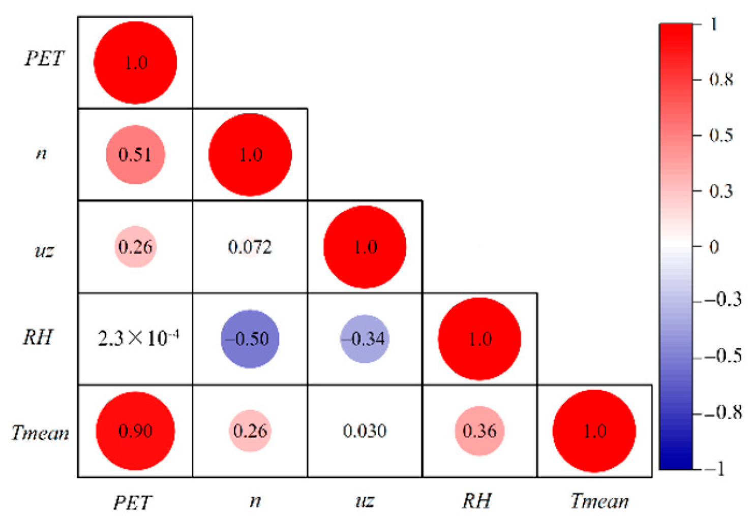
The input scenarios of the machine learning model were determined according to the magnitude of the nonparametric Spearman correlation coefficient between the daily PET and the input factors, i.e., the average daily air temperature (Tmean, °C), daily average relative humidity (RH, %), wind speed at 10 m height (uz, m s−1), and sunshine hours (n, h). First, the Spearman correlation coefficient between the daily PET in the YRB and each of the input factors was determined (Figure 2), and the factor with the largest correlation coefficient relative to daily PET was selected as Scenario 1. Scenarios 2–4 were determined by adding the next highest correlation factor on the basis of Scenario 1. The final results are shown in Table 2.

3.1.2. Performance of the Machine Learning Model during Training and Testing Periods

To evaluate the accuracy of the training and testing period models, according to the selected four scenarios, the evaluation indices (R2, NSE, and KGE) of three machine learning models in eight sub-basins were calculated under each scenario. Each box plot was generated based on the evaluation results of each model in 115 meteorological stations, as shown in Figure 3 and Figure 4.
According to the results of the training period (Figure 3), the performance of every model continued to improve with increased input data. No significant differences were observed in terms of accuracy between the machine learning models under each input scenario. According to the results of the testing period (Figure 4), the evaluation indicators of the three models fluctuated considerably with increased input data, with outliers in multiple sub-basin stations, indicating that the model became less robust with increased input variables when simulating different meteorological stations, possibly because the model was overfit with a large number of input factors during the training period [58].
A comprehensive comparison of the performances of the SVR, RF, and ELM models in the training and testing periods under the four scenarios shows that Scenario 2 is optimal, taking the average temperature and sunshine hours as the input variables of PET. The accuracy of Scenario 2 during the testing period was better than that of Scenario 1, with fewer abnormal data point in the simulation results than in Scenarios 3–4. The models performed well for Scenario 2, with a median KGE of more than 0.82 at 115 stations.

3.1.3. Stability Evaluation of Machine Learning Models

To evaluate the stability of the model, the absolute change in RMSE during the testing period was compared to the training period under different climate scenarios for the three machine learning models, as previously reported by Huang et al. [27]. The smaller the absolute value of RMSE, the better the stability of the model.
According to analysis from the perspective of four climate scenarios (Figure 5), the sum of RMSE absolute values in the four scenarios of SVR, RF, and ELM models were 6.66, 18.37, 61.05, 90.61 (SVR); 6.33, 12.51, 50.88, and 64.98 (RF) and 6.13, 20.23, 75.57, and 90.89 (ELM), respectively. The results show that the stability of the three models decreased with increased input factors, and the stability of Scenario 3 differed considerably from that of Scenario 2. In the scenarios in which the input factor is greater than or equal to 2, the RF model performs best, with the strongest stability among the three investigated models.
According to the results of the eight sub-basins in the hydrological division among the three scenarios except Scenario 1, the median variation in RMSE in sub-basin VII was the smallest among other sub-basins. Although the stability of the model in Scenario 2 was worse than that in Scenario 1, the value of RMSE between the testing and training periods of each sub-basin varied from −0.21 to 0.77, and the stability results were acceptable. The RMSE value in Scenario 3 varied from −0.09 to 2.22, with poor stability results. Therefore, the simulated data in Scenario 2, with Tmean and n as input variables of PET, were selected for the three machine learning models in the subsequent comparative analysis. In this scenario, the accuracy of the model simulation was balanced by the number of input factors.

3.2. Spatiotemporal Variation of PET

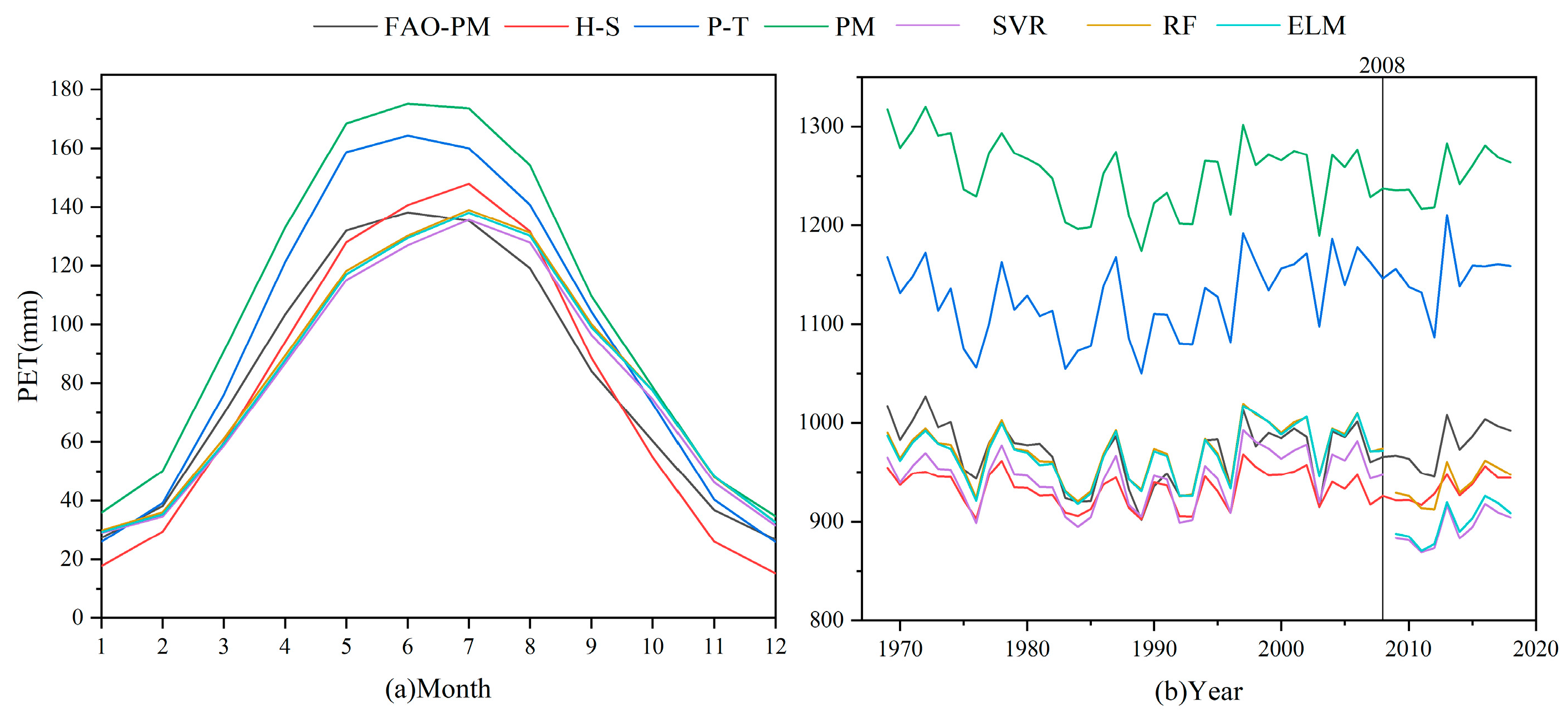
In this section, we qualitatively analyze the trend changes of empirical and machine learning models under Scenario 2 on month and annual scales (Figure 6). The average statistical results for data from the same month data in all years are shown in Figure 6a. The results of different models show that PET in the YRB exhibits a significant intra-annual change trend, and its value reaches the maximum in summer (June, July, and August), accounting for 40–45% of the total PET during the year, followed by spring, autumn, and winter. In the empirical models, the monthly average results of the temperature-based H-S model fluctuated in the FAO-PM model, that is, in the summer with higher temperature, the simulation results were higher than the FAO-PM results, with increased deviation with lower temperatures in the remaining seasons. The radiation-based P-T model overestimated PET, but the calculation results of the model in winter (December, January, and February) were consistent with those of the FAO-PM model. The PM model based on the comprehensive method considerably overestimated all monthly statistics. The results of the three machine learning models were most consistent with the recommended method. Compared with FAO-PM, the simulation results presented lower values for February to June, with smaller overestimation in other months.
The multiyear average PET results (Figure 6b) show a fluctuating trend in the YRB (FAO-PM). In the empirical models, the H-S model underestimated throughout the study period, the P-T and PM models considerably overestimate, and the annual value results differed considerably from those obtained using the recommended method. In the machine learning models, the simulation results of RF and ELM performed well during the training period (1969–2008), and the results for multiple periods were close those obtained with the FAP-PM model. Although the SVR simulation results presented with low values, they also captured the trend in the data. In the testing period (2009–2018), the simulation results of the machine learning models were lower than those in the training period.
According to the above analysis, with respect to the overall change trend, the empirical and machine learning models showed a similar trend compared with the standard FAO-PM model. However, the P-T and PM are numerically overestimated, and the H-S model underestimated. Although the results of the three machine learning models were consistent with those obtained with the FAO-PM model, the training period results of the machine learning model were better than those in the testing period.
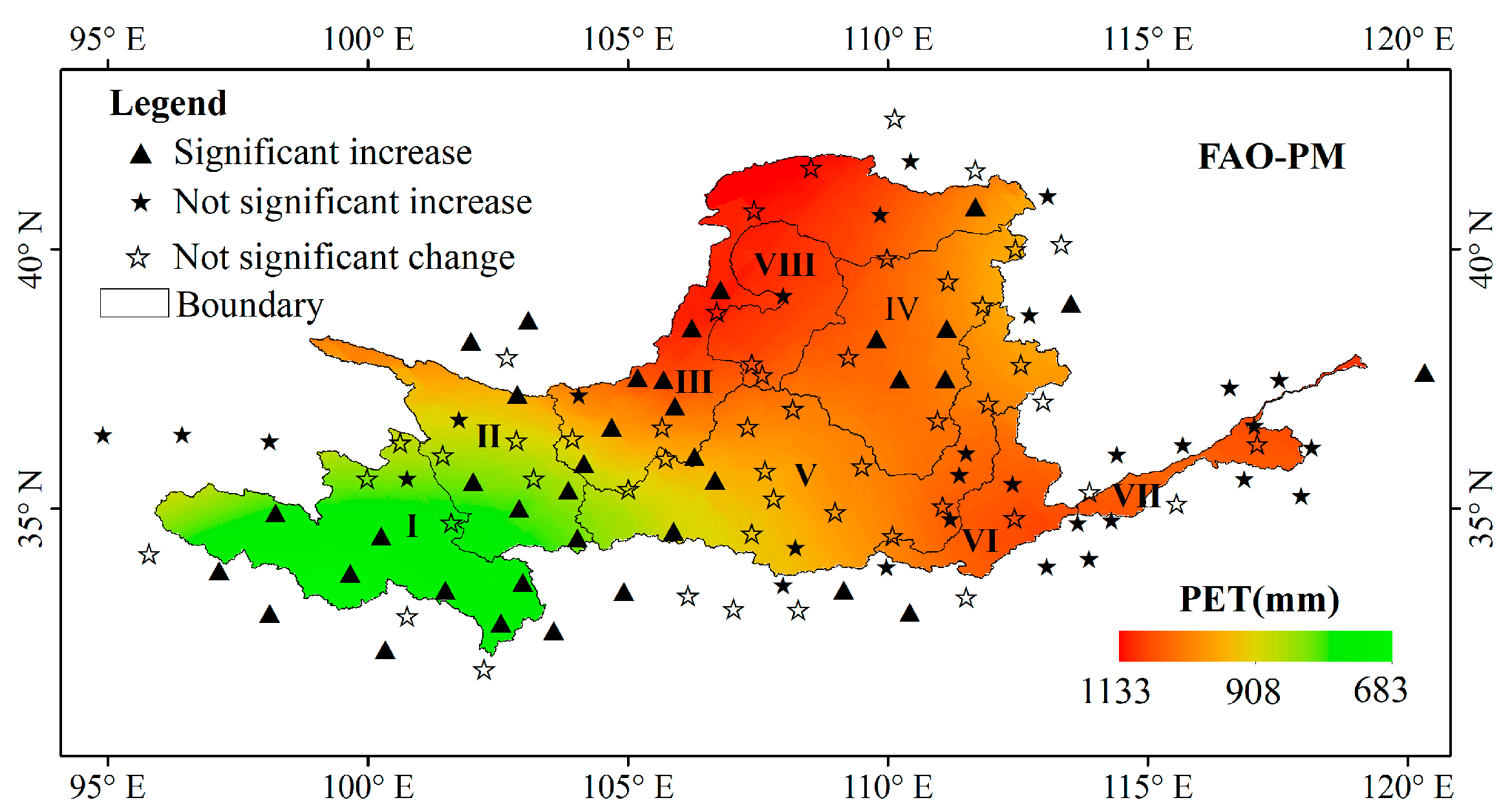
The trends (Mann–Kendall) of annual PET values from 1969 to 2018 in 115 stations were analyzed, and we applied Kriging spatial interpolation of multiyear average PET in the YRB. The results are shown in Figure 7. PET in the YRB is high in the east and low in the west and gradually decreases from the east to the west. Among the 115 stations, the number of stations showing a significant increase (p < 0.05) accounted for 32.2% of the total number of stations, and most of these stations are located in the upper YRB; most of the stations that showed a significant decrease are located in the lower YRB.

3.3. Comparative Analysis of Machine Learning Models and Empirical Models

In order to further verify the applicability of machine learning, in this section, we compare the results of machine learning models under Scenario 2 with those obtained using the three empirical models. In the comparative analysis, PBIAS and AICc were used for evaluation (Table 3). PBIAS (%) was used to describe the deviation of the model simulation results from the true value. Because the types and quantities of meteorological factors input by various PET empirical models and machine learning models differed considerably, we calculated the AICc value, and the number of input factors was considered when comparing the accuracy of the models.
According to the PBIAS values, the three machine learning models all minorly underestimated in the entire study area, and RF performed best among the three models. The simulation results of the radiation-based P-T and synthesis method PM considerably overestimated in most sub-basins. Whether the simulation results of the temperature-based H-S model were overestimated is related to the simulation area. Based on the results of the whole research period, considering the deviation of the model results (PBIAS) and the number of model simulation accuracy and variables (AICc), the machine learning models were generally better than the empirical models, and the RF and ELM models achieved the best performance, indicating that the machine learning models have strong applicability for PET simulation in the YRB.
The analysis results of the above evaluation indices are consistent with the results of qualitative analysis (Figure 6), with the results of the evaluation indicators demonstrating the performance of the model in different sub-basins of the YRB in more detail. Considering the simulation accuracy of the model and the number of variables, the three best-performing models were RF > ELM > H-S.

4. Discussion

4.1. Comparative Analysis of PET Calculation Models

The empirical and machine learning models were qualitatively and quantitatively compared. According to the research results in the YRB, due to the strong regional applicability of the empirical models, both the P-T and PM models considerably overestimated, whereas the H-S model fluctuated with respect to the FAO-PM results. These results are consistent with the development conditions of the original model. Studies have shown that the radiation-based P-T model was developed for a warm and humid climate [6], which explains the poor performance of the method in the arid and semi-arid YRB. The PM method computes the PET for an open water surface, so it usually obtains the highest value [1]. The temperature-based H-S model was originally developed for dry climates [59], which is consistent with the FAO’s suggestion that the H-S model can be used to estimate PET in areas with only the lowest and highest temperatures [17]. Studies have shown that H-S models often overestimate or underestimate PET [60], so they are more suitable for the estimation of PET in the YRB than the P-T and PM models.
According to the results obtained in the study area, the machine learning models are more regionally applicable than the empirical models and require less meteorological input to achieve satisfactory model accuracy. As the most commonly used machine learning algorithm, the SVR model performed poorly in this study, although previous studies using this method in different study areas resulted in to the opposite conclusion [27,61]. The RF in the six models showed overall performance [62], indicating that the RF model in the YRB is more applicable with fewer overfitting problems [46]. In a commercial farm study in Florida, Granata [61] found that RF provided the best predictions with a limited number of input variables (net solar radiation, wind speed, mean relative humidity, and mean temperature). The ELM model is slightly less accurate than the RF model but performed better in some sub-basins in this study and was proven efficient in previous studies [63]. Researchers strongly recommend using this algorithm in arid and semi-arid areas.
According to the above analysis, the machine learning models are generally better than the empirical models [58]. Furthermore, none of the six methods selected in this study achieve optimal results in all cases [53], and there is no scientific consensus with respect to the optimal algorithm to estimate PET. Therefore, selecting a calculation model without comparison of PET in the Yellow River Basin will result in a considerable error in the research results.

4.2. Factors Affecting the Accuracy of Machine Learning Estimation

Analysis of variance (ANOVA) can be used to test which factors have significant effects on the results. In this study, ANOVA was used to test which factors, input scenarios, machine learning models, or their interaction exerted significant effects on the accuracy of PET simulation.
Table 4 shows the ANOVA results. The F crit (3.4903) of scenario factors at a 95% confidence level was lower than the F value (31.0516) calculated for different scenarios, whereas the F crit (3.8853) of model factors at a 95% confidence level was higher than the F value (3.6784) calculated by different models. The F crit (2.9961) of the interaction between scenarios and models at the 95% confidence level was higher than F value (2.0540). According to the above analysis results, the accuracy of PET simulation in the YRB depends on the input scenarios of different meteorological factors.
Our results are consistent with those reported in previous studies [61,64], indicating that the performance of machine learning models varies depending on the number of inputs and the predicted length of time. Generally, the accuracy of models with complete meteorological factors is better than that of models with incomplete input data [28,65]. However, due to economic conditions, geographical location, and other factors, meteorological stations in some areas do not collect data on all meteorological factors. In such cases, in order to use machine learning algorithms to simulate local PET, the accuracy of the input factors can be controlled the factors that are important for PET simulation can be selected as inputs to control the simulation results of the model [27,66,67].
Using machine learning to simulate PET in the YRB, the model’s accuracy depends on the input of meteorological factor data. A lack of the most important factor data in PET simulation results in a significant decline in model performance. Therefore, the appropriate input factors should be selected when using machine learning for PET modeling.

4.3. Importance of Meteorological Factors of Altitude and Drought Index for PET Predictions

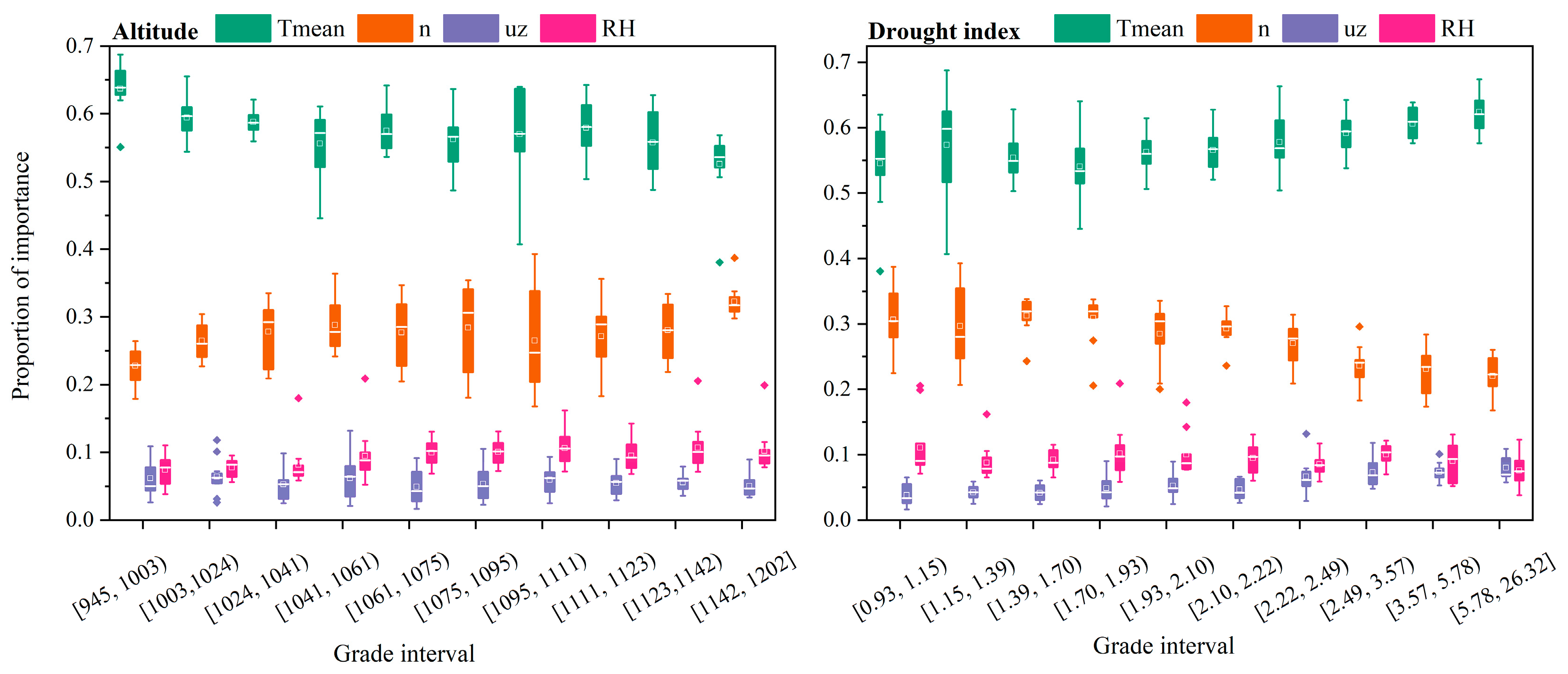
With respect to the importance of meteorological factors in PET simulation at different altitudes and drought indices in the YRB, the altitudes and drought indices in the YRB were divided into deciles. Figure 8 shows the proportion of importance of four meteorological factors in PET simulation under 10 altitude (left) and drought index (right) grade intervals. The results show that Tmean accounted for the largest proportion, followed by n, and the sum of the two accounted for 82–88% of the total importance index [68]. Previous studies revealed that temperature has a considerable impact on PET in the constructed PET model [69]. Zhao et al. [70] also found that the contribution rate of n to PET was second only to Tmean in multiple climatic zones in China.
The importance of Tmean shows a decreasing trend with increased altitude, whereas that of n shows the opposite trend. The importance of uz and RH shows a small downward and upward trend with increased altitude, indicating that the importance of the Tmean factor in the simulation of PET in regions with high altitudes (source region of the Yellow River) is lower than that in regions with relatively low altitudes (lower Yellow River). The n factor is more important in higher altitude areas [71].
Previous studies mostly discussed the relationship between PET and drought [72,73], as well as the impact of climate change on drought [70,74]. In this study, we focused on the degree of influence of meteorological factors on PET simulation at different drought index stations (Figure 8, right). The importance of Tmean exhibits an increasing tendency with an increase in the drought index, whereas the importance of n decreases, indicating that the importance of Tmean is higher in dry areas than in humid areas, and the importance of n is opposite. For uz and RH, with a total importance proportion of less than 20%, uz shows a small upward trend with increased drought index, whereas the importance of RH changed little in different drought index levels.
According to the above analysis, the changing trend of the same meteorological factor differs depending on the altitude and drought index grade interval, although the overall importance ranking is unchanged, namely Tmean > n > RH > uz. The results of the importance index differ from those of the Spearman correlation coefficient, as the simulation of PET is a complex, nonlinear calculation process [65,75].

5. Conclusions

(1)
Average temperature (Tmean) and sunshine hours (n) can be used as input combinations of the model to obtain satisfactory daily potential evapotranspiration (PET) predictions when lacking complete meteorological variables and using machine learning to estimate PET in the Yellow River basin (YRB).
(2)
A comparison of the selected machine learning and empirical models shows that machine learning models limited to two input variables generally perform better than empirical models, and the empirical models usually overestimate or underestimate. Among the six models, random forest (RF) performs best in general, followed by extreme learning machine; none of the six methods selected in this study are optimal for prediction in all watersheds.
(3)
Analysis of variance results show that the accuracy of PET simulation in the YRB depends on the input scenario of different meteorological factors at the significance level of 0.05 relative to machine learning models.
(4)
According to the importance index provided by RF simulation, Tmean is the most important factor, followed by n. However, the influence of Tmean on PET gradually decreases with increased altitude and gradually increases with a drier climate, whereas the influence of n shows the opposite trend. The importance of relative humidity is higher than that of wind speed, in contrast to the ranking calculated by the Spearman correlation coefficient with PET, indicating that the simulation of PET is a complex, nonlinear calculation process.
The results of this study will help researchers who select appropriate meteorological factors to calculate PET in the YRB and provide a reference for researchers to simulate or evaluate the performance of different models. Furthermore, under global warming climate conditions, decision makers can use these results to manage agricultural water resources in the YRB. In this research, only three commonly used machine learning algorithms were selected for comparison, and a comparative study of multiple algorithms should be conducted in the future.

Author Contributions

Conceptualization, J.L. and K.Y.; methodology, J.L.; software, J.L. and L.J.; validation, K.Y., P.L. and X.Z.; formal analysis, J.L.; resources, K.Y., Z.Y. and Y.Z.; data curation, J.L.; writing—original draft preparation, J.L. and K.Y.; writing—review and editing, J.L., K.Y. and L.J.; visualization, J.L.; supervision, K.Y.; project administration, P.L.; funding acquisition, K.Y. All authors have read and agreed to the published version of the manuscript.

Funding

This research was supported by the National Natural Science Foundations of China (Grant Nos. 52079104, U2040208, and 51979290), the Ningxia Water Conservancy Science and Technology Project (SBZZ-J-2021-12) and Basic research Fund Project of China Institute of Water Resources and Hydropower Research (SE0145B022022).

Institutional Review Board Statement

Not applicable.

Informed Consent Statement

Not applicable.

Data Availability Statement

This study includes the daily data of 115 meteorological stations in the Yellow River Basin provided by the China Meteorological Data Sharing Service Center (http://data.cma.cn/, accessed on 10 June 2019). The spatial distribution of meteorological stations is shown in Figure 1.

Conflicts of Interest

The authors declare no conflict of interest.

References

  1. Zhou, J.; Wang, Y.; Su, B.; Wang, A.; Tao, H.; Zhai, J.; Kundzewicz, Z.W.; Jiang, T. Choice of potential evapotranspiration formulas influences drought assessment: A case study in China. Atmos. Res. 2020, 242, 104979. [Google Scholar] [CrossRef]
  2. Wang, W.; Shao, Q.; Peng, S.; Xing, W.; Yang, T.; Luo, Y.; Yong, B.; Xu, J. Reference evapotranspiration change and the causes across the Yellow River Basin during 1957–2008 and their spatial and seasonal differences. Water Resour. Res. 2012, 48. [Google Scholar] [CrossRef]
  3. Zhang, B.; Xu, D.; Liu, Y.; Chen, H. Review of multi-scale evapotranspiration estimation and spatio-temporal scale expansion. Trans. Chin. Soc. Agric. Eng. 2015, 31, 8–16. (In Chinese) [Google Scholar]
  4. Kim, D.; Chun, J.A.; Ko, J. A hybrid approach combining the FAO-56 method and the complementary principle for predicting daily evapotranspiration on a rainfed crop field. J. Hydrol. 2019, 577, 123941. [Google Scholar] [CrossRef]
  5. Liu, X.; Yang, W.; Zhao, H.; Wang, Y.; Wang, G. Effects of the freeze-thaw cycle on potential evapotranspiration in the permafrost regions of the Qinghai-Tibet Plateau, China. Sci. Total Environ. 2019, 687, 257–266. [Google Scholar] [CrossRef] [PubMed]
  6. Lu, J.; Sun, G.; McNulty, S.G.; Amatya, D.M. A Comparison of Six Potential Evapotranspiration Methods for Regional Use in the Southeastern United States. J. Am. Water Resour. As. 2005, 41, 621–633. [Google Scholar] [CrossRef]
  7. Bai, P.; Liu, X.; Yang, T.; Li, F.; Liang, K.; Hu, S.; Liu, C.J.J. Assessment of the influences of different potential evapotranspiration inputs on the performance of monthly hydrological models under different climatic conditions. J. Hydrometeorol. 2016, 17, 2259–2274. [Google Scholar] [CrossRef]
  8. Band, L.E.; Mackay, D.S.; Creed, I.F.; Semkin, R.; Jeffries, D. Ecosystem processes at the watershed scale: Sensitivity to potential climate change. Limnol. Oceanogr. 1996, 41, 928–938. [Google Scholar] [CrossRef]
  9. Hay, L.E.; McCabe, G.J. Spatial Variability in Water-Balance Model Performance in the Conterminous United States. J. Am. Water Resour. Assoc. 2002, 38, 847–860. [Google Scholar] [CrossRef]
  10. Xiang, K.; Li, Y.; Horton, R.; Feng, H. Similarity and difference of potential evapotranspiration and reference crop evapotranspiration—A review. Agr. Water Manag. 2020, 232, 106043. [Google Scholar] [CrossRef]
  11. Li, S.; Kang, S.; Zhang, L.; Zhang, J.; Du, T.; Tong, L.; Ding, R. Evaluation of six potential evapotranspiration models for estimating crop potential and actual evapotranspiration in arid regions. J. Hydrol. 2016, 543, 450–461. [Google Scholar] [CrossRef]
  12. Um, M.J.; Kim, Y.; Park, D.; Jung, K.; Wang, Z.; Kim, M.M.; Shin, H. Impacts of potential evapotranspiration on drought phenomena in different regions and climate zones. Sci. Total Environ. 2020, 703, 135590. [Google Scholar] [CrossRef] [PubMed]
  13. Lang, D.; Zheng, J.; Shi, J.; Liao, F.; Ma, X.; Wang, W.; Chen, X.; Zhang, M. A Comparative Study of Potential Evapotranspiration Estimation by Eight Methods with FAO Penman–Monteith Method in Southwestern China. Water 2017, 9, 734. [Google Scholar] [CrossRef]
  14. Grismer, M.E.; Orang, M.; Snyder, R.; Matyac, R. Pan Evaporation to Reference Evapotranspiration Conversion Methods. J. Irrig. Drain Eng. 2002, 128, 180–184. [Google Scholar] [CrossRef]
  15. Yang, Y.; Chen, R.; Han, C.; Liu, Z. Evaluation of 18 models for calculating potential evapotranspiration in different climatic zones of China. Agr. Water Manag. 2021, 244, 106545. [Google Scholar] [CrossRef]
  16. Bormann, H. Sensitivity analysis of 18 different potential evapotranspiration models to observed climatic change at German climate stations. Clim. Chang. 2010, 104, 729–753. [Google Scholar] [CrossRef]
  17. Allan, R.G.; Pereira, L.S.; Raes, D.; Smith, M. Crop evapotranspiration-Guidelines for computing crop water requirements—FAO Irrigation and drainage paper 56. FAO Rome 1998, 300, D05109. [Google Scholar]
  18. Xu, C.-y.; Gong, L.; Jiang, T.; Chen, D.; Singh, V.P. Analysis of spatial distribution and temporal trend of reference evapotranspiration and pan evaporation in Changjiang (Yangtze River) catchment. J. Hydrol. 2006, 327, 81–93. [Google Scholar] [CrossRef]
  19. Fan, J.; Wang, X.; Wu, L.; Zhou, H.; Zhang, F.; Yu, X.; Lu, X.; Xiang, Y. Comparison of Support Vector Machine and Extreme Gradient Boosting for predicting daily global solar radiation using temperature and precipitation in humid subtropical climates: A case study in China. Energ. Convers. Manag. 2018, 164, 102–111. [Google Scholar] [CrossRef]
  20. Mattar, M.A. Using gene expression programming in monthly reference evapotranspiration modeling: A case study in Egypt. Agr. Water Manag. 2018, 198, 28–38. [Google Scholar] [CrossRef]
  21. Taormina, R.; Chau, K.-W. Data-driven input variable selection for rainfall–runoff modeling using binary-coded particle swarm optimization and Extreme Learning Machines. J. Hydrol. 2015, 529, 1617–1632. [Google Scholar] [CrossRef]
  22. Acharya, N.; Shrivastava, N.A.; Panigrahi, B.K.; Mohanty, U.C. Development of an artificial neural network based multi-model ensemble to estimate the northeast monsoon rainfall over south peninsular India: An application of extreme learning machine. Clim. Dynam. 2013, 43, 1303–1310. [Google Scholar] [CrossRef]
  23. Deo, R.C.; Tiwari, M.K.; Adamowski, J.F.; Quilty, J.M. Forecasting effective drought index using a wavelet extreme learning machine (W-ELM) model. Stoch. Env. Res. Risk A 2016, 31, 1211–1240. [Google Scholar] [CrossRef]
  24. Feng, Y.; Cui, N.; Zhao, L.; Hu, X.; Gong, D. Comparison of ELM, GANN, WNN and empirical models for estimating reference evapotranspiration in humid region of Southwest China. J. Hydrol. 2016, 536, 376–383. [Google Scholar] [CrossRef]
  25. Tabari, H.; Kisi, O.; Ezani, A.; Hosseinzadeh Talaee, P. SVM, ANFIS, regression and climate based models for reference evapotranspiration modeling using limited climatic data in a semi-arid highland environment. J. Hydrol. 2012, 444–445, 78–89. [Google Scholar] [CrossRef]
  26. Antonopoulos, V.Z.; Antonopoulos, A.V. Daily reference evapotranspiration estimates by artificial neural networks technique and empirical equations using limited input climate variables. Comput. Electron. Agric. 2017, 132, 86–96. [Google Scholar] [CrossRef]
  27. Huang, G.; Wu, L.; Ma, X.; Zhang, W.; Fan, J.; Yu, X.; Zeng, W.; Zhou, H.J.J. Evaluation of CatBoost method for prediction of reference evapotranspiration in humid regions. J. Hydrol. 2019, 574, 1029–1041. [Google Scholar] [CrossRef]
  28. Salam, R.; Islam, A.R.M.T. Potential of RT, bagging and RS ensemble learning algorithms for reference evapotranspiration prediction using climatic data-limited humid region in Bangladesh. J. Hydrol. 2020, 590, 125241. [Google Scholar] [CrossRef]
  29. Wen, X.; Si, J.; He, Z.; Wu, J.; Shao, H.; Yu, H. Support-Vector-Machine-Based Models for Modeling Daily Reference Evapotranspiration with Limited Climatic Data in Extreme Arid Regions. Water Resour. Manag. 2015, 29, 3195–3209. [Google Scholar] [CrossRef]
  30. Yamaç, S.S.; Todorovic, M. Estimation of daily potato crop evapotranspiration using three different machine learning algorithms and four scenarios of available meteorological data. Agr. Water Manag. 2020, 228, 105875. [Google Scholar] [CrossRef]
  31. AR6 Climate Change 2021: The Physical Science Basis Intergovernmental Panel. 2021. Available online: https://www.ipcc.ch/report/ar6/wg1/ (accessed on 17 May 2022).
  32. Jia, L.; Yu, K.; Li, Z.; Li, P.; Zhang, J.; Wang, A.; Ma, L.; Xu, G.; Zhang, X. Temporal and spatial variation of rainfall erosivity in the Loess Plateau of China and its impact on sediment load. CATENA 2022, 210, 0341–8162. [Google Scholar] [CrossRef]
  33. Ullah, I.; Ma, X.; Ren, G.; Yin, J.; Iyakaremye, V.; Syed, S.; Lu, K.; Xing, Y.; Singh, V.P. Recent Changes in Drought Events over South Asia and Their Possible Linkages with Climatic and Dynamic Factors. Remote Sens. 2022, 14, 3219. [Google Scholar] [CrossRef]
  34. Ullah, I.; Saleem, F.; Iyakaremye, V.; Yin, J.; Ma, X.; Syed, S.; Hina, S.; Asfaw, T.G.; Omer, A. Projected Changes in Socioeconomic Exposure to Heatwaves in South Asia Under Changing Climate. Earth’s Future 2022, 10, e2021EF002240. [Google Scholar] [CrossRef]
  35. Ullah, I.; Ma, X.; Yin, J.; Omer, A.; Habtemicheal, B.A.; Saleem, F.; Iyakaremye, V.; Syed, S.; Arshad, M.; Liu, M. Spatiotemporal characteristics of meteorological drought variability and trends (1981–2020) over South Asia and the associated large-scale circulation patterns. Clim. Dyn. 2022, 1–24. [Google Scholar] [CrossRef]
  36. Xi, J. Speech at the symposium on ecological protection and quality development in Speech at the symposium on ecological protection and quality development in the Yellow River Basin. Water Resour. Dev. Manag. 2019, 1–4. (In Chinese) [Google Scholar] [CrossRef]
  37. Guo, H. Sustainable development and ecological environment protection in high-quality development of the Yellow River Basin. J. Humanit. 2020, 17–21. (In Chinese) [Google Scholar] [CrossRef]
  38. Zhao, W.; Ji, X.; Liu, H. Progresses in Evapotranspiration Research and Prospect in Desert Oasis Evapotranspiration Research. Arid Zone Res. 2011, 28, 463–470. (In Chinese) [Google Scholar]
  39. Zhao, Y.; He, F.; He, G.; Li, H.; Wang, L.; Chang, H.; Zhu, Y. Review the Phenomenon of Yellow River Cutoff from a Whole Perspective and ldentification of Current Water Shortage. Yellow River 2020, 42, 42–46. (In Chinese) [Google Scholar]
  40. Wang, W.; Zhang, Y.; Tang, Q. Impact assessment of climate change and human activities on streamflow signatures in the Yellow River Basin using the Budyko hypothesis and derived differential equation. J. Hydrol. 2020, 591, 125460. [Google Scholar] [CrossRef]
  41. Liu, F.; Chen, S.; Dong, P.; Peng, J. Temporal and spatial variation of runoff in the Yellow River Basin in the past 60 years. J. Geogr. Sci. 2012, 22, 1013–1033. [Google Scholar] [CrossRef]
  42. Ringler, C.; Cai, X.; Wang, J.; Ahmed, A.; Xue, Y.; Xu, Z.; Yang, E.; Jianshi, Z.; Zhu, T.; Cheng, L.; et al. Yellow River basin: Living with scarcity. Water Int. 2010, 35, 681–701. [Google Scholar] [CrossRef]
  43. Miao, C.; Ni, J.; Borthwick, A.G.L.; Yang, L. A preliminary estimate of human and natural contributions to the changes in water discharge and sediment load in the Yellow River. Glob. Planet Chang. 2011, 76, 196–205. [Google Scholar] [CrossRef]
  44. Hargreaves, G.H.; Samani, A.Z. Reference Crop Evapotranspiration from Temperature. Appl. Eng. Agric. 1985, 1, 96–99. [Google Scholar] [CrossRef]
  45. Priestley, C.; Taylor, R.J. On the Assessment of Surface Heat Flux and Evaporation Using Large Scale Parameters. Mon. Weather Rev. 1972, 100, 81–92. [Google Scholar] [CrossRef]
  46. Penman, H.L. Vegtation and Hydrology. Soil Sci. 1963, 96, 357. [Google Scholar] [CrossRef]
  47. Douglas, E.M.; Jacobs, J.M.; Sumner, D.M.; Ray, R.L. A comparison of models for estimating potential evapotranspiration for Florida land cover types. J. Hydrol. 2009, 373, 366–376. [Google Scholar] [CrossRef]
  48. Cortes, C.; Vapnik, V. Support-vector networks. Mach. Learn. 1995, 20, 273–297. [Google Scholar] [CrossRef]
  49. Chen, J.T.; Zhong, J.; Xie, Y.C.; Cai, C.Y. Text Classification Using SVM with Exponential Kernel. Appl. Mech. Mater. 2014, 519–520, 807–810. [Google Scholar] [CrossRef]
  50. Breiman, L. Random Forests. Mach. Learn. 2001, 45, 5–32. [Google Scholar] [CrossRef]
  51. Wang, S.; Lian, J.; Peng, Y.; Hu, B.; Chen, H. Generalized reference evapotranspiration models with limited climatic data based on random forest and gene expression programming in Guangxi, China. Agr. Water Manag. 2019, 221, 220–230. [Google Scholar] [CrossRef]
  52. Huang, G.-B.; Zhu, Q.-Y.; Siew, C.-K. Extreme learning machine: Theory and applications. Neurocomputing 2006, 70, 489–501. [Google Scholar] [CrossRef]
  53. Dou, X.; Yang, Y. Applications of Machine Learning Methods in Modeling Carbon and Water Fluxes of Terrestrial Ecosystems. Ph.D. Thesis, China University of Mining University, Beijing, China, 2018. [Google Scholar]
  54. Gupta, H.V.; Kling, H.; Yilmaz, K.K.; Martinez, G.F. Decomposition of the mean squared error and NSE performance criteria: Implications for improving hydrological modelling. J. Hydrol. 2009, 377, 80–91. [Google Scholar] [CrossRef]
  55. Meles, M.B.; Goodrich, D.C.; Gupta, H.V.; Shea Burns, I.; Unkrich, C.L.; Razavi, S.; Guertin, D.P. Multi-criteria, time dependent sensitivity analysis of an event-oriented, physically-based, distributed sediment and runoff model. J. Hydrol. 2021, 598, 126268. [Google Scholar] [CrossRef]
  56. Yu, K.-x.; Zhang, X.; Xu, B.; Li, P.; Zhang, X.; Li, Z.; Zhao, Y. Evaluating the impact of ecological construction measures on water balance in the Loess Plateau region of China within the Budyko framework. J. Hydrol. 2021, 601, 126596. [Google Scholar] [CrossRef]
  57. Moral, F.J.; Paniagua, L.L.; Rebollo, F.J.; García-Martín, A. Spatial analysis of the annual and seasonal aridity trends in Extremadura, southwestern Spain. Theor. Appl. Climatol. 2017, 130, 917–932. [Google Scholar] [CrossRef]
  58. Dong, J.; Zhu, Y.; Jia, X.; Shao, M.a.; Han, X.; Qiao, J.; Bai, C.; Tang, X. Nation-scale reference evapotranspiration estimation by using deep learning and classical machine learning models in China. J. Hydrol. 2022, 604, 127207. [Google Scholar] [CrossRef]
  59. Martínez-Cob, A.; Tejero-Juste, M. A wind-based qualitative calibration of the Hargreaves ET0 estimation equation in semiarid regions. Agr. Water Manag. 2004, 64, 251–264. [Google Scholar] [CrossRef]
  60. Khoob, R.A. Comparative study of Hargreaves’s and artificial neural network’s methodologies in estimating reference evapotranspiration in a semiarid environment. Irrig. Sci. 2008, 26, 253–259. [Google Scholar] [CrossRef]
  61. Granata, F. Evapotranspiration evaluation models based on machine learning algorithms—A comparative study. Agr. Water Manag. 2019, 217, 303–315. [Google Scholar] [CrossRef]
  62. Fernández Delgado, M.; Cernadas García, E.; Barro Ameneiro, S.; Amorim, D.G. Do we need hundreds of classifiers to solve real world classification problems. J. Mach. Learn. Res. 2014, 15, 3133–3181. [Google Scholar] [CrossRef]
  63. Abdullah, S.S.; Malek, M.A.; Abdullah, N.S.; Kisi, O.; Yap, K.S. Extreme Learning Machines: A new approach for prediction of reference evapotranspiration. J. Hydrol. 2015, 527, 184–195. [Google Scholar] [CrossRef]
  64. Laaboudi, A.; Mouhouche, B.; Draoui, B. Neural network approach to reference evapotranspiration modeling from limited climatic data in arid regions. Int. J. Biometeorol. 2012, 56, 831–841. [Google Scholar] [CrossRef] [PubMed]
  65. Fan, J.; Yue, W.; Wu, L.; Zhang, F.; Cai, H.; Wang, X.; Lu, X.; Xiang, Y. Evaluation of SVM, ELM and four tree-based ensemble models for predicting daily reference evapotranspiration using limited meteorological data in different climates of China. Agr. Forest Meteorol. 2018, 263, 225–241. [Google Scholar] [CrossRef]
  66. Chen, H.; Huang, J.J.; McBean, E. Partitioning of daily evapotranspiration using a modified shuttleworth-wallace model, random Forest and support vector regression, for a cabbage farmland. Agr. Water Manag. 2020, 228, 105923. [Google Scholar] [CrossRef]
  67. Mohammadi, B.; Mehdizadeh, S. Modeling daily reference evapotranspiration via a novel approach based on support vector regression coupled with whale optimization algorithm. Agr. Water Manag. 2020, 237, 106145. [Google Scholar] [CrossRef]
  68. Feng, Y.; Jia, Y.; Zhang, Q.; Gong, D.; Cui, N. National-scale assessment of pan evaporation models across different climatic zones of China. J. Hydrol. 2018, 564, 314–328. [Google Scholar] [CrossRef]
  69. Wu, L.; Huang, G.; Fan, J.; Ma, X.; Zhou, H.; Zeng, W. Hybrid extreme learning machine with meta-heuristic algorithms for monthly pan evaporation prediction. Comput. Electron. Agric. 2020, 168, 105115. [Google Scholar] [CrossRef]
  70. Zhao, L.; Zhao, X.; Pan, X.; Shi, Y.; Qiu, Z.; Li, X.; Xing, X.; Bai, J. Prediction of daily reference crop evapotranspiration in different Chinese climate zones: Combined application of key meteorological factors and Elman algorithm. J. Hydrol. 2022, 610, 127822. [Google Scholar] [CrossRef]
  71. Li, Y.; Qin, Y.; Rong, P. Evolution of potential evapotranspiration and its sensitivity to climate change based on the Thornthwaite, Hargreaves, and Penman–Monteith equation in environmental sensitive areas of China. Atmos. Res. 2022, 273, 106178. [Google Scholar] [CrossRef]
  72. Ma, T.; Liang, Y.; Lau, M.K.; Liu, B.; Wu, M.M.; He, H.S. Quantifying the relative importance of potential evapotranspiration and timescale selection in assessing extreme drought frequency in conterminous China. Atmos. Res. 2021, 263, 105797. [Google Scholar] [CrossRef]
  73. Shi, L.; Feng, P.; Wang, B.; Liu, D.L.; Yu, Q. Quantifying future drought change and associated uncertainty in southeastern Australia with multiple potential evapotranspiration models. J. Hydrol. 2020, 590, 125394. [Google Scholar] [CrossRef]
  74. Wang, Y.; Wang, S.; Zhao, W.; Liu, Y. The increasing contribution of potential evapotranspiration to severe droughts in the Yellow River basin. J. Hydrol. 2022, 605, 127310. [Google Scholar] [CrossRef]
  75. Wu, L.; Fan, J. Comparison of neuron-based, kernel-based, tree-based and curve-based machine learning models for predicting daily reference evapotranspiration. PLoS ONE 2019, 14, e0217520. [Google Scholar] [CrossRef] [PubMed] [Green Version]
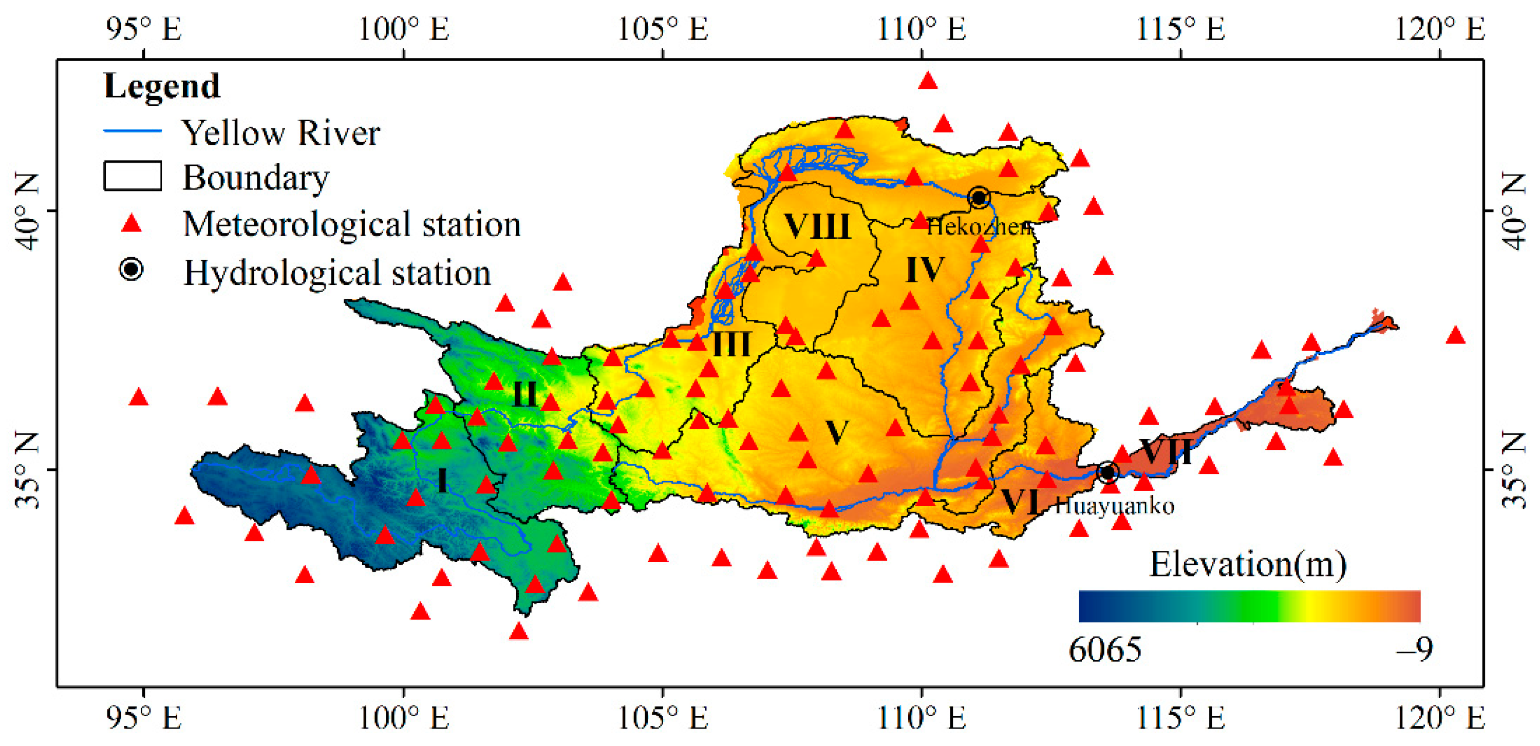
Figure 1. The locations of meteorological stations and sub-basins used in this study. Note: The numbers in the figure represent each sub-basin; I represents the watershed above Longyangxia, II represents Longyangxia-Lanzhou, III represents Lanzhou-Hekouzhen, IV represents Hekouzhen-Longmen, V represents Longmen-Sanmenxia, VI represents Sanmenxia-Huayuankou, VII represents the watershed below Huayuankou, and VIII represents Neiliu District.
Atmosphere 13 01467 g001
Figure 2. Spearman correlation coefficient between PET and meteorological factors.
Atmosphere 13 01467 g002
Figure 3. Evaluation indicators of three machine learning models under the four scenarios in the training period.
Atmosphere 13 01467 g003
Figure 4. Evaluation indicators of three machine learning models under the four scenarios in the testing period.
Atmosphere 13 01467 g004
Figure 5. Change in RMSE during the testing and training periods under four scenarios for the three machine learning models.
Atmosphere 13 01467 g005
Figure 6. The month (a) and annual (b) variation trend of PET in the Yellow River Basin.
Atmosphere 13 01467 g006
Figure 7. Multiyear PET and spatial variation trends of 115 stations in the Yellow River basin.
Atmosphere 13 01467 g007
Figure 8. The importance proportion of four meteorological factors in PET simulation under different altitude (left) and drought index (right) grade intervals.
Atmosphere 13 01467 g008
Table 1. Empirical models and formulae for calculating PET.
MethodCategoryAbbreviationFormulation
Hargreaves–SamaniTemperature-based methodH-S P E T = [ 0.0023 R a ( T m e a n + 17.8 ) ( T max T min ) ] 0.5 λ (2)
Priestley–TaylorRadiation-based methodP-T P E T = 1.26 ( R n G ) λ Δ Δ + γ (3)
PenmanCombination methodPM P E T = Δ ( R n G ) λ ( Δ + γ ) + γ Δ + γ 6.43 ( 1 + 0.53 u 2 ) ( e s e a ) λ (4)
Note: P E T is potential evapotranspiration (mm day−1), Ra is extraterrestrial radiation (MJ m−2 day−1), Tmax is daily maximum temperature (°C), Tmin is daily minimum temperature (°C), and λ is latent heat of vaporization (kPa °C−1).
Table 2. Input scenarios for machine learning models.
Input ScenarioModel Input Factor(s)
Scenario 1Tmean
Scenario 2Tmean + n
Scenario 3Tmean + n + uz
Scenario 4Tmean + n + uz + RH
Table 3. Evaluation indicators of daily PET in machine learning model and empirical models from 1969 to 2018.
Sub-BasinEvaluation IndicatorSVRRFELMH-SP-TPM
IPBIAS−1.95−1.05−1.305.9029.9035.90
AICc−2.17−2.13−2.160.511.770.59
IIPBIAS−4.80−2.90−3.80−0.2532.8031.70
AICc−1.47−1.53−1.353.322.150.72
IIIPBIAS−4.90−1.00−1.80−13.703.8026.10
AICc−1.13−1.02−1.210.631.590.81
IVPBIAS−6.15−1.50−2.10−8.3014.5526.30
AICc−1.07−1.17−1.180.381.980.76
VPBIAS−5.00−1.80−3.100.4027.0029.00
AICc−1.33−1.40−1.360.171.740.74
VIPBIAS−7.7−3.6−6.1−0.6016.2026.70
AICc−0.54−0.97−0.250.281.600.78
VIIPBIAS−2.950.600.400.157.5528.30
AICc−1.41−1.42−1.430.251.130.88
VIIIPBIAS−5.80−1.10−2.2−15.558.2024.60
AICc−1.06−1.08−1.160.801.920.76
Note: Light blue indicates the model with the smallest deviation in the sub-basin, and light orange represents the AICc value of the model with best performance in the sub-basin.
Table 4. ANOVA results for scenarios and models.
SSdfMSF Valuep-ValueF Crit
Scenarios0.165430.055131.05166.15 × 10−63.4903
Models0.013120.00653.67840.05683.8853
Scenarios and models0.021960.00362.05400.13602.9961
Inside0.0213120.0018
Total0.221723
Note: SS, sum of squares; df, degrees of freedom; MS, mean square.
Publisher’s Note: MDPI stays neutral with regard to jurisdictional claims in published maps and institutional affiliations.