Comparative Analysis of the Observation Bias and Error Characteristics of AGRI and AHI Data for Land Areas in East Asia

Abstract

Observation bias and error characteristics are the preconditions for the effective assimilation of observation data. In this paper, the bias and error characteristics of the AHI (Advanced Himawari Imager (AHI) and AGRI (Multi-Channel Advanced Geostationary Orbit Radiation Imager (AGRI) data are compared and analyzed, with an emphasis on the observations obtained from land areas. The results show that the observation errors of the two instruments for the ocean area have a good channel consistency over ocean areas, which are all with errors of about 0.6 K; however, the bias and error are significantly affected by the land-surface types and terrain heights over land. For most of the AHI channels, the bias in urban-area bias is smaller than that of those of other surface types, while that of the AGRI data exhibits just the opposite trend, with obviously larger biases in urban areas. However, the observation errors of these two instruments in urban areas are significantly smaller than those of other surface types. The biases of the two instruments do not extensively change much with the terrain height, only slightly decreasing when the height is above 1000 m; however, the observation errors increase obviously with the increase of terrain heights. The difference between the two instruments is that the observation error of the AHI data tends to be stable and stabilizes above 1000 m, while that of the AGRI data is relatively stable below 500 m. The observation errors of the CO₂-sensitive channels of the two instruments over the land areas are obviously smaller than those of other near-surface channels, which may indicate that the data obtained in these two CO₂ channels have good application prospects for assimilation over land.

1. Introduction

For short-term weather forecasting, the accuracy of the initial values is an important factor that affects the accuracy of the numerical weather forecasting results. Data assimilation technology is an important method for improving the accuracies of the initial values input to numerical models. A model’s initial field improvements are mainly induced through data assimilation methods using abundant meteorological observation information. Among many meteorological observation data sources, satellite observations are not affected by regional limitations, and this feature compensates for the defects of conventional observation data areas. Satellite observation data account for 98% of the meteorological observation data and have become the most important observation data source for reducing errors in operational numerical forecasts [1].

At present, effectively assimilated satellite radiation data can be divided into two categories: polar-orbiting satellite data, collected in sun-synchronous orbits, and geostationary satellite data, collected in geosynchronous orbits. As a single polar-orbiting satellite can cover the whole world only twice a day, when simulating fast-moving convective weather systems, polar-orbiting satellite data have the shortcomings of insufficient temporal and spatial coverage, and only stationary satellites can provide continuous observation data representing a certain area.

Data assimilation research on static infrared imagers has also received widespread attention from meteorologists. Especially with the successful launch of a new generation of geostationary meteorological satellites with advanced infrared imagers in China, the United States and Japan, where data assimilation research involving infrared imagers onboard geostationary satellites has been greatly promoted. Many meteorologists have tried to assimilate the data collected in the infrared channels of global or regional geostationary satellite imagers [2,3,4,5,6,7], thus greatly improving the accuracy of numerical weather forecasts. The research of Honda et al., Zhang et al., Minamide et al. and Xu et al. [8,9,10,11] also confirmed that the assimilation of geostationary satellite data can significantly improve the analysis and forecasting of thermal variables and wind fields and can also improve the numerical weather forecasting effects of typhoons and other high-impact weather events.

Although infrared imager data contain several high-altitude water vapor channels and near-ground channels, more attention has been given to the water vapor channels [3,11,12,13], while only a few studies have focused on assimilating the data collected at low levels [14,15,16,17], resulting in a considerable amount of observation data being wasted around land areas. Compared to the data assimilation research performed in ocean areas, the data assimilation methods of data collected from the geostationary satellite imagers over land areas are more complicated. In addition, the vegetation type, terrain height and prevalence of small-scale weather systems lead to increased uncertainties in the surface emissivity and surface temperature characterizing the background field, thus significantly increasing the complexity of the observation errors and deviation estimations of terrestrial near-surface channels. This feature represents one of the main difficulties faced when assimilating the data collected at the near-surface channels of geostationary satellite infrared imagers over land areas.

Data assimilation methods are based on the difference between observed data and the background field; these differences are combined with the observation error and background field error characteristics to realize the optimal adjustment of the background field. In data assimilation research, it is very important to quantitatively characterize the deviation and error characteristics of the measured values relative to “real” data. In principle, data assimilation requires the observation errors of observed data to be unbiased, so it is necessary to fully understand the deviation characteristics of the utilized data accurately and remove these deviations using deviation-correction methods [18]. These observation errors are an important basis for setting the initial weights of observed data in data assimilation research [19]. However, the greatest difficulty when assimilating the data collected over land is that the observation errors are large and difficult to estimate accurately [20,21].

Defining the characteristics of errors and deviations in each imager channel is a prerequisite for effectively assimilating satellite data. Many meteorologists have also analyzed the error characteristics of infrared imager data in detail. Zhuge et al. [21] used the International Geosphere-Biosphere Programme (IGBP), UW_HER and the Combined Advanced Spaceborne Thermal Emission and Reflection Radiometer (ASTER) and Moderate-resolution Imaging Spectroradiometer (MODIS) Emissivity database over Land—High Spectral Resolution (CAMEL_HSR) datasets as inputs in the radiative transmission model. They compared and analyzed the deviation characteristics of the Advanced Himawari Imager (AHI) under three sets of conditions and deviation characteristics corresponding to different underlying surface types; this work was beneficial to the subsequent development of data assimilation involving the AHI surface-sensitive channels. Qu et al. [22], based on the use of the reanalysis data provided by the European Centre for Medium-Range Weather Forecasts (ECMWF) in their ECMWF Re Analysis version 5 (ERA5) product, which were used as inputs in the rapid radiative transfer model, Radiative Transfer for the Television Infrared Observation Satellite (TIROS) Operational Vertical Sounder (TOVS) (RTTOV), analyzed the deviation and distribution characteristics between the simulated data and the data observed at the Advanced Geostationary Radiation Imager (AGRI) infrared channels, demonstrating that shortwave infrared channels are greatly affected by surface reflection conditions, and large deviations occur. Geng [23] and others also used the RTTOV model but applied the Global Forecast System (GFS) analysis data as the inputs and adopted a variational deviation-correction scheme, thus laying a foundation for the assimilation and application of the infrared channel emissivity data of AGRI in the mesoscale models. Tang et al. [17], based on the use of the Final (FNL) and ERA5 datasets as inputs, applied the newly developed fast radiative transfer model, called the Atmospheric Radiation Measurement (ARM) model, to study the observation-minus-background (O−B) deviation characteristics of the AGRI infrared band.

Although many studies have analyzed the error characteristics of the satellite data collected over ocean and land areas, most past works have simply counted the average error and bias characteristics of the infrared imager data collected over ocean and land surfaces. In contrast to the uniformity of the ocean’s underlying surface, the satellite data error and deviation characteristics in land areas are also affected by the terrain height and vegetation type. Although numerical models can simulate temperature and humidity profile information at the troposphere layer and above, great uncertainties still arise when simulating land-surface temperatures. The terrain height and surface type are important factors that affect the accuracy of the ground temperatures participating in the background field. Due to the complexity of underlying surface types, existing surface emissivity datasets also contain large errors [21]. Therefore, this paper focuses on performing bias and error analyses for each channel over land areas. In this research, we classify the error and bias characteristics of the AHI and AGRI data collected for land areas from the two aspects of terrain height and vegetation type to provide a reference for the assimilation of the near-surface channel data recorded by geostationary satellite infrared imagers over land areas.

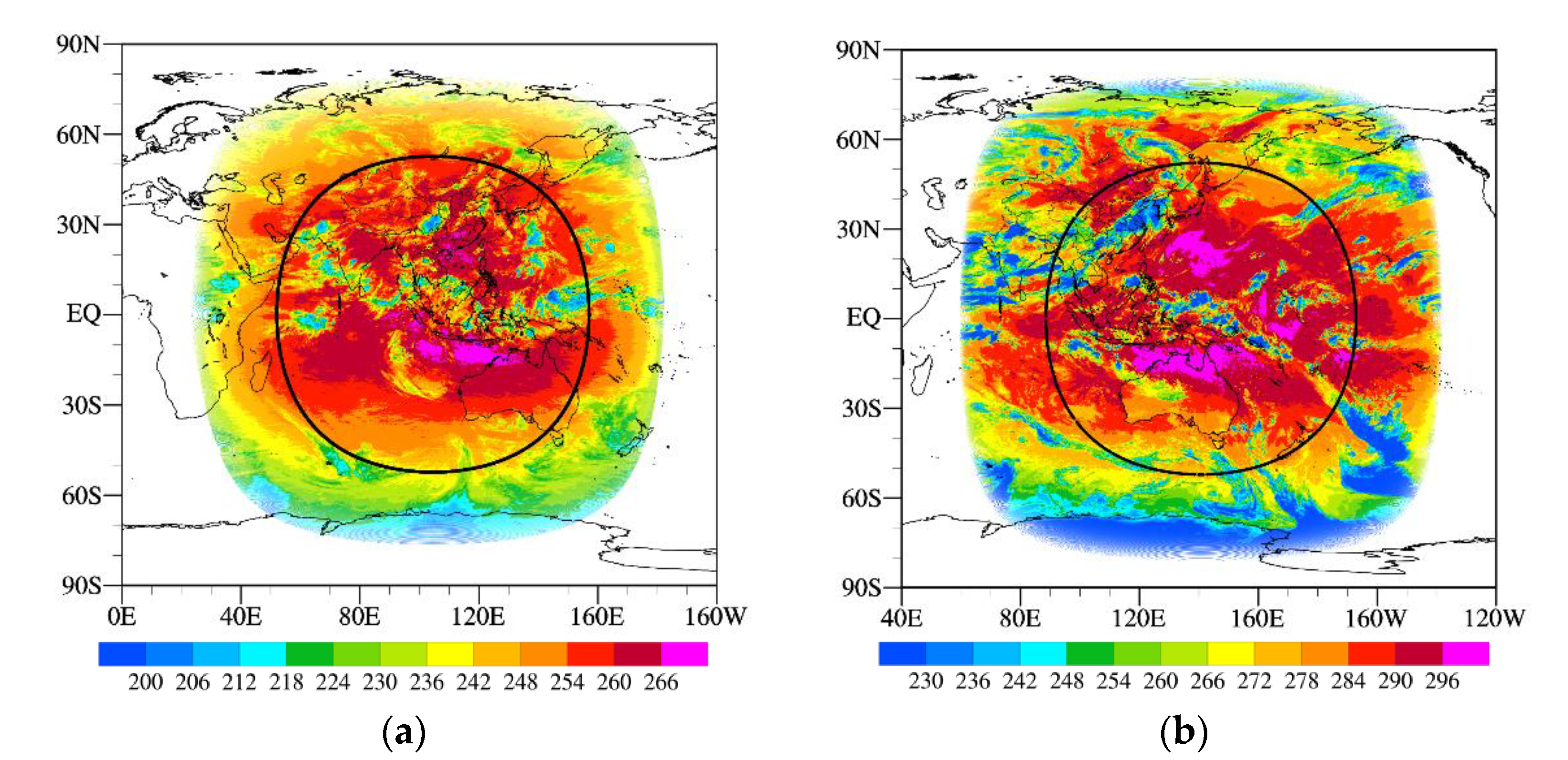
The specific structure of this paper is as follows. The Section 2 introduces the data sources and overviews of the analyzed images. The Section 3 shows the spatial distributions of the observed and simulated brightness temperatures. The Section 4 compares and discusses the O-B mean and standard deviation values of the AHI and AGRI datasets on different channels and under varying land and sea conditions. The Section 5 further analyzes the influence of different vegetation types and terrain heights on the O-B mean and standard deviation values. Finally, the Section 6 provides the main conclusions.

2. Information and Methods

Since the mid-1970s, when the United States and the European Union launched the first geostationary satellites into space, the load observation accuracies of the geostationary meteorological satellites in various countries have continuously improved [24]. At present, American geostationary operational meteorological satellites (GOES) have developed to the fourth generation; the GOES-R satellite, the first satellite in this series, is equipped with an advanced baseline imager (ABI) with 16 channels [25]. The latest generation of Japanese geostationary orbit satellites is the “Himawari” series. The main observation instrument onboard this series of satellites is the Advanced Himawari Imager (AHI), which also has a 16-channel imaging capability [26]. The main function and performance of the AHI are similar to those of the ABI. The Fengyun-4 series (FY-4) meteorological satellite, with a geostationary orbit developed by China, is equivalent to the latest-generation GOES-R series in the United States and is equipped with the AGRI sensor that collects data with a multi-pass scanning ability. The AGRI on FY-4A has 14 imaging channels, comparable to the international level [27]. Because the observation ranges of the AHI and AGRI overlap greatly and the main functions and performances of these imaging channels are similar, in this study, we simultaneously analyze the infrared imaging error characteristics of the AHI and AGRI over the land areas of China and further clarify the deviations in the infrared imager data collected from land areas and the stability of the error characteristics through comparisons and mutual verifications.

2.1. Introduction of AGRI and AHI

The FY-4A is the first satellite in the FY-4 geostationary-orbit constellation; this satellite adopts a three-axis stable attitude-control system. Compared to the FY-2 meteorological satellites, which undergo stable spin, the FY-4A satellite has achieved leap-forward development in both function and performance. At present, it is located 35,786 km above the equator at 104.7° E [26]. The FY-4A is equipped with a new generation of multichannel scanning imaging radiometers (the AGRI) developed in China. There are clear differences in usage and division of labor among the 14 AGRI data channels, including 2 visible bands, 4 near-infrared bands and 8 infrared bands. The AGRI provides full-disk observations at 15-minute intervals. The minimum spatial resolution of the AGRI 0.65-µm band is 0.5 km; that of both the 0.47- and 0.83-µm bands is 1 km; and that of the 1.378, 1.61, 2.23 µm and high-resolution 3.75-µm bands is 2 km. For the low-resolution 3.75-µm band and the remaining infrared bands, the AGRI observation resolution is 4 km. Among these channels, channels 8, 11, 12 and 13 in the band are sensitive to the land surface. Bands 9 and 10 of the AGRI are located in the moisture absorption zone; thus, these two channels are moisture-sensitive, with peak weights at 350 hPa and 500 hPa, respectively. Channel 14 is located in the carbon dioxide absorption band.

The Japanese third-generation geostationary meteorological satellites are referred to as the Himawari series; two satellites have been successfully launched at present. The Himawari 8 satellite carries an advanced imager, the AHI [27]. The main function and performance of the AHI are equivalent to those of the ABI carried by the GOES-R satellite developed in the United States; the AHI has 16 channels for imaging capability, including 3 visible light channels, 3 near-infrared channels and 10 infrared channels. The AHI can scan the whole viewing disk every 10 min and even every 2.2 min for Japan and some specific target areas. This satellite is located at 140.7° E above Tokyo, and its observation range can reach 120 × 120 (80° E–20° W, 60° N–60° S), thus providing good observations over most parts of China. The 10 infrared channels can be used for AHI data assimilation, among which channels 8, 9 and 10 are water vapor detection channels with corresponding central wavelengths of 6.30 μm, 6.95 μm and 7.35 μm, respectively; the weight functions of these three channels reach peak values at 377 hPa, 457 hPa and 587 hPa, respectively, while the weight functions of the other seven infrared channels reach their peak values at the surface. Channel 12 is an ozone-sensitive channel, and its weighting function exhibits a second peak in the stratosphere. Channel 16 is located in the carbon dioxide absorption band.

Table 1. Characteristics of each channel parameter of the AHI and AGRI.

Himawari-8 AHI, Japan				FY-4A AGRI, China
Channel Number	Center Wavelength	Channel	Resolution/km	Channel Number	Center Wavelength	Channel	Resolution /km
7	3.85	0.22	2.0	8	3.75 L	0.50	4.0
8	6.24	0.37	2.0	9	6.25	0.90	4.0
9	6.95	0.12	2.0	10	7.1	0.4	4.0
10	7.35	0.17	2.0	11	8.5	1.0	4.0
11	8.60	0.32	2.0	12	10.7	0.8	4.0
12	9.63	0.18	2.0	13	12.0	1.0	4.0
13	10.45	0.30	2.0	14	13.5	0.6	4.0
14	11.20	0.2	2.0
15	12.35	0.30	2.0
16	13.30	0.2	2.0

lists the infrared channel characteristics of the AHI and AGRI, including the center wavelength, channel width and resolution characteristics. From the comparison, it can be found that many channels in the AHI and AGRI correspond to each other.

Table 2. Similar functional channels between the AHI and AGRI.

Instrument	Water Vapor Detection Channels	Surface-Sensitive Channels	CO2 Absorption Channels
AHI	Channels 8, 9, and 10	Channels 7, 11, 12, 13, 14, and 15	Channel 16
AGRI	Passage Channels 9, and 10	Channels 8, 11, 12, and 13	Channel 14

lists the water vapor detection channels, surface-sensitive channels and CO₂ absorption channels that correspond to these two imagers.

2.2. Introduction to the WRF Model System

Considering that these two types of satellite data may be assimilated in the data reanalysis process, which will lead to a biased conclusion, the hourly forecast of the Weather Research and Forecast-Advanced Research WRF (WRF-ARW) model is used as background in this study [28]. Take the FNL data as the initial forecast field, make a 6-h forecast, adopt the hourly forecast results in the 6–12-h period as the input data for the rapid radiation model, and obtain the simulation results using AHI and AGRI data. We believe that the research results, based on such background fields, are also conducive to the practical assimilation application of the two kinds of data because the WRF model is also a model often used in other studies.

The WRF model is a new-generation mesoscale regional climate model system jointly developed by the National Center for Atmospheric Research (NCAR) and the National Centers for Environmental Prediction (NCEP). We selected version 4.1, WRF-ARWV4.1, in this work. The horizontal mode resolution of this model is 6 km, and the model contains 61 vertical layers from the land surface to the top of the model at approximately 50 hPa. The total grid point pattern in 3D space contains 600 × 600 × 61 points. The WRF Single-Moment (WSM3) microphysical scheme [29], Kain–Fritsch cumulus parameterization scheme [30,31] and Yonsei planetary boundary layer scheme [32] are selected for parameterization.

3. Spatial Distribution of Brightness Temperatures in East Asia

3.1. Cloud Detection Method

Infrared radiation is sensitive to clouds. Because the errors induced by the influence of clouds on radiation estimations are relatively large, to better clarify the deviation and error characteristics of the observation data, we selected only clear-sky data for the analysis in this study. Regarding the AHI data, the cloud detection method, developed by Zhuge and Zou [33], which depends only on infrared data, was selected. A cloud detection process was carried out on the observation data, and clear-sky observation data were obtained. Compared to the MODIS cloud detection process, the “correct classification probabilities” of this cloud detection method were found to be 91.94% and 92.59% in the daytime and nighttime over land, respectively. Regarding the AGRI data, due to the great uncertainties associated with the cloud detection products of AGRI, we used the cloud detection products matched with the MODIS sensor onboard the Aqua/Terra satellite to obtain clear-sky data in this study [17].

3.2. Coverage of the AGRI and AHI

Figure 1 shows the spatial distributions of the monthly average brightness temperature observed by the AGRI, channel 14 (the CO₂ channel), at about 0000 UTC on 1 July 2019, and by the AHI, channel 16, at about 0000 UTC on 1 July 2016. Only data collected at the satellite scanning angles of less than 60 degrees were selected here to ensure the simulation accuracy of the radiative transfer model. The black curves show the domain with a satellite zenith angle of less than 60°.

The FY-4A satellite is stationed at 104.7° E, effectively covering most of China. The maximum observed brightness temperature of channel 14 is approximately 268 K, while the minimum temperature is 200 K. Figure 1b shows the spatial distributions of the brightness temperature observed by channel 16 of the AHI at about 0000 UTC on 1 July 2016. The brightness temperature of the AHI, channel 16, is basically higher than that of AGRI’s channel 14. The Himawari satellite is located at 140.7° E. There are also significant differences in the coverage of the data of the two satellites with zenith angles of less than 60°. The 60-degree zenith angle of the AHI can reach 50° E in the west of the coverage area, while that of the AHI is around 90° E. This study mainly focuses on the observation bias and error of data in land areas, so the research domain is selected as 90–150° E, 10–45° N. Due to the limitation of data storage space, we selected the AHI data in July 2016 and AGRI data in July 2019 for this comparative study. Although the times of the two data are different, their statistical characteristics should be independent of the data time.

4. Bias and Error Analyses of AGRI and AHI

To reveal the average error characteristics of the two analyzed instruments, the average and standard deviation O-B values of the data recorded by the two instruments were calculated by using the hourly AHI and AGRI data collected over a one-month period. Figure 2 shows the statistical results characterizing the deviation characteristics and observation errors of the data collected in the AHI channels 7–11 and 13–16 in July 2016 and the data collected in the AGRI channels 8–14 in July 2019 over both the ocean and land. The brightness temperatures recorded by AHI channel 12 are also affected by the ozone content in the upper layer, resulting in relatively large simulation errors, so these channel data are not considered here. Due to difficulties in obtaining data, the AHI and AGRI data collected in the same year could not be selected; however, both analyzed datasets were recorded during the summer season in July. As shown in Figure 3, the errors of the upper water vapor channel data are obviously smaller than those of other near-surface channels. The deviations of the AHI water vapor channels (channels 8, 9, and 10) and AGRI water vapor channels (channels 9 and 10) are positive; the average deviation of the AHI water vapor channels over the ocean is approximately 0.1 K, while that on land is larger, at approximately 0.3 K. These results are similar to those obtained by Zhuge et al. [21]. The average deviation of the water vapor channels of the AGRI (channels 9 and 10) is approximately 0.7 K over the ocean, while that on land is slightly reduced to approximately 0.5 K. These results are similar to the findings of Tang et al. [17].

Among the other near-surface channels, the AHI channels 11–16 show obvious negative deviations over both ocean and land areas, with deviations of approximately −0.1 K, and the land deviations are much larger than the ocean deviations; the maximum deviation can reach −0.3 K. However, channel 7, which has a lower frequency than the other channels, exhibits positive deviations. Channel 8, which has a similar frequency as the AGRI, also exhibited positive deviations, and those of the CO₂-sensitive channel 14 were also positive, while the other channels exhibited negative deviations; however, the land deviations of the AGRI were smaller than those over the ocean surface area, representing a marked difference from the AHI findings.

In the data assimilation process, the O-B standard deviation is an important parameter used to specify the observation error. The underlying surface has a significant influence on the O-B standard deviation. The O-B standard deviations obtained for both instruments were much larger over the land areas than over the ocean areas. In ocean areas, the average standard deviation of all AHI channels is approximately 0.5 K, while that of the AGRI data is approximately 0.7 K. Basically, no obvious difference was found between the upper water vapor channels and the near-surface channels, and these stable observation errors are one of the reasons why assimilating the data recorded in each channel over the ocean areas is more likely to have positive effects than assimilating the data collected over land areas [19].

In contrast, over land areas, the O-B standard deviations of the upper water vapor channels are slightly increased; the average O-B standard deviation of the AHI channels 8–10 increased to 0.8 K, and that of the AGRI channels is also increased to 0.9 K. However, the O-B standard deviations of other near-surface channels increase significantly. For the AHI, the standard deviations of the surface-sensitive channels (channels 7, 11, 13, 14 and 15) increase significantly over land (blue bars in Figure 3), all reaching approximately 1.1 K. In contrast, the O-B standard deviation of CO₂-sensitive channel 16 increases slightly, to approximately 0.8 K; this characteristic is similar to those seen for the water vapor channels, possibly suggesting that the brightness temperature simulation involving channel-16 data is less affected by the surface variables than the simulations involving other channels. For the AGRI data, the O-B standard deviations of the near-ground channels over land increased obviously, reaching values above 1.5 K, but the O-B standard deviation of channel 14 was relatively small, at only approximately 1.3 K.

Geostationary satellites are relatively stationary with respect to the Earth and observe the Earth from more than 30,000 m in outer space. Since it is a single-instrument observation mode, with the different zenith angles corresponding to the observation data, the observation paths of the satellites are bound to be significantly different, which easily leads to differences in the observation performance of the instruments. In the radiation transmission mode, biases caused by the zenith angles have been corrected. However, in order to further clarify this, the variation characteristics of the land data bias and the error of channel 10 of the two satellites with the zenith angle are also given in Figure 3. The two high-altitude channels are selected to better show the influence of the zenith angles. It can be seen in Figure 3 that the data from the AGRI is between 30° and 60°, while the zenith angle of the AHI data is basically above 40°. Ignoring those zenith angles with fewer data, the bias of the two channels is relatively stable. Although the observation error slightly increases with the increase of the zenith angle after the zenith angle is greater than 40°, the increase is only about 0.2 K.

The bias and standard deviation of the O-B represent the statistical characteristics of the instrument performance, and the stability of the statistical results is very important for practical application. In order to further clarify the spatial stability of the above statistical results, the spatial distribution of the O-B standard deviation of the CO₂ channels of the two instruments is given in Figure 4. It can be seen in the figure that the spatial consistency of standard deviations in the ocean area is high, and the overall error is smaller than that in the land area. This is consistent with the previous analysis results, which also prove the good representation of the observation error in the ocean area. However, it is not true for the observation error in the land area; this varies dramatically from region to region. The biggest difference with the ocean surface is that the land surface has different terrain heights and vegetation types. Therefore, the following further analyzes the observation bias and error with the vegetation type and terrain height.

5. Variation Characteristics of the O-B Means and Standard Deviations with Terrain Height and Vegetation Type

5.1. Data Deviations and Errors under Different Vegetation Types

To further refine the bias and error characteristics of the two kinds of imager data collected over land areas, the changes in the O-B mean and standard deviation values obtained for each channel’s different underlying surface type and terrain height conditions are further analyzed in the following paragraphs.

Figure 5 shows the distribution numbers of different underlying surface types in East Asia in summer. To ensure the stability of the statistical results, only four types of vegetation corresponding to large amounts of instrument-collected data—city, grassland, pine forest and broadleaf pine forest vegetation—are selected for further research. Although many bare-soil data points exist in the instrument datasets, bare-soil distribution data are missing at some topographic heights. Thus, bare soil is not selected among the analyzed vegetation types.

Figure 6 shows the O-B mean and standard deviation values of different AHI and AGRI channels under the four selected vegetation types. Among the different vegetation types, the O-B average and standard deviation of each channel differ significantly. For the AHI, the underlying surface type has a more obvious influence on the near-surface channels, while channels 13–14 in pine forests exhibit positive deviations contrary to the average result. It is worth noting that the deviation and observation error of each near-surface channel are obviously lower than those of the other channels in urban areas, even those of the high-altitude water vapor channel. The deviations of the AGRI data in the urban and pine forest areas are obviously different from those in the grassland and broadleaf forest areas. The deviations of each channel in the urban and pine forest areas are positive, while those in the grassland and broadleaf pine forest areas are positive only in the water vapor channels (channels 9 and 10) and CO₂-sensitive channels and are negative in the other near-surface channels. The urban-area deviations are significantly higher than those of other vegetation types, which is the opposite of the AHI. Similar to the AHI, the O-B standard deviation of each AGRI channel is lower in urban than other vegetation types, while the standard deviation of each AGRI channel is also low in pine forest areas.

The O-B mean and standard deviation values obtained for various vegetation types exhibited obvious differences, indicating that in actual assimilation applications, the deviation-correction and observation weight settings in land-based data assimilation need to be adjusted according to the vegetation type, especially in urban areas. Both analyzed instruments show small observation errors, and such small errors are often ignored in current land infrared-imager-based data assimilation work. In addition, it is worth noting that the AGRI and AHI have a common feature; that is, the O-B standard deviation of the CO₂-sensitive channel is obviously smaller than those of other channels, regardless of the vegetation type. Qin’s [16] research also proved that the AHI CO₂ detection channel observation error, derived over land areas, was less affected by surface variables, allowing for small observation errors to be obtained and thus indicating that the data collected in this channel can be directly applied to data assimilations over land areas. The comparison results derived herein also show that the AGRI channel 14 data obtained over the land areas also have data assimilation potential.

5.2. O-B Average and Standard Deviation Values at Different Terrain Heights

In addition to the underlying surface type, the changeable terrain height also greatly influences the brightness temperature simulation results. Terrain effects not only increase the uncertainty of the background surface temperature and wind-field values but also further amplify the influence of the background field and surface emissivity errors during the data assimilation process. Therefore, the influence of the terrain height on the observation deviation and error characteristics is further analyzed in this section.

Figure 7 shows a topographic height distribution map spanning East Asia. Except for the Qinghai-Tibet Plateau and the northern region, the topographic heights in East Asia are mostly below 2000 m. Considering the different coverages of the two kinds of analyzed observation data, to ensure a good overlap between the two instruments, in the study, we selected only the area east of 105° E for our comparative analysis; the topographic heights of this area are basically concentrated below 2000 m.

By considering the similarities in the near-surface channel characteristics, for clarity, only some channels are selected for this comparative analysis. It is known from the above analysis that, compared to other surface-sensitive channels, the deviation and error characteristics of the CO₂-sensitive channels of the AHI and AGRI differ obviously from those of other near-surface channels. Therefore, only the CO₂ detection channels and one of the near-surface channels are selected from the two analyzed instruments to compare the observation deviation and error characteristics. Here, channel 14 and channel 16 of the AHI are selected, while channel 12 and channel 14 of the AGRI are selected.

Figure 8 shows the variations in the O-B standard deviations of AHI’s channels 14 and 16 with terrain height under the four vegetation types. It can be clearly seen that even for the same vegetation type, there are great O-B characteristic differences among the different terrain heights. Channel 14 maintains a positive deviation in the pine forest areas of approximately 0.4 K, but at heights above 900 m, this deviation rapidly decreases from the positive deviation to approximately 0.2 K. Under the other vegetation types, the negative deviation below 1000 m is approximately −0.4 K and decreases slightly after 1000 m. The four vegetation types captured by channel 16 all exhibit negative deviations that fluctuate slightly with the terrain height and are all stable between −0.7 K and −0.5 K. The standard deviations of the observation errors are consistent among different vegetation types and increase with increasing terrain heights. Channel 14 tends to stabilize after 1000 m at approximately 1.6 K, while channel 16 continues to increase with increasing terrain heights. At approximately 1500 m, the standard deviations of the grassland and urban areas are both 1.1 K, while those of the pine forest and broadleaf pine forest areas are 1.3 K. It can be seen from this result that in the land data assimilation research, deviations and observation errors need to be adjusted, not only according to the underlying vegetation types but while considering the influence of terrain heights.

The O-B mean and standard deviation values of the two AGRI channels also obviously differ with the changes in terrain height (Figure 9). The O-B deviations of channel 12 in the urban and pine areas exhibit little change with the varying terrain heights; the deviation in the urban areas is kept at −0.2 K to 0.2 K, and for the pine areas, it is approximately 0.4 K. However, the bias in the other two vegetation types greatly changes with the height of the terrain. From a height of 700 m, the bias gradually decreases with increasing heights. Under all the terrain heights, the O-B bias of channel 14 in all four vegetation types is positive, except in the pine forest area, and the bias also shows decreasing trends at heights of greater than 700 m. It should be pointed out that in the broadleaf forest area with a height of 300–400 m, the O-B has a large negative bias. Further analysis shows that this may be related to the sample size. More data are needed for statistical analyses in this height range.

The O-B standard deviations of the two channels also obviously increase with increasing terrain heights, but the standard deviations gently change below 500 m, similar to the conclusion by Qu et al. [22]. From the comparison of these two channels, it can be seen that the variation amplitude of channel 14 is small, and the error is low, maintained between 1.1 K and 1.4 K throughout the whole variation process. The standard deviation of channel 12 is significantly larger than that of channel 14; the lowest deviation is 1.2 K at 500 m, and the standard deviations of the grassland and pine forest areas can reach 1.8 K at approximately 1500 m. The AGRI results further verify that the observation errors increase over land areas with increasing terrain heights. At the same time, the comparison between the two channels further verifies that the observation error of channel 14, which is sensitive to CO₂, is obviously smaller over land areas than those of the other near-surface channels, further proving the potential of using channel-14 data in land data assimilation research.

6. Conclusions and Discussion

The infrared imager data collected by geostationary satellites with high spatiotemporal resolutions can well meet the initialization requirements of a high-resolution numerical model. Although much research has been done on the data assimilation of geostationary satellite infrared imagery, most of those past studies have focused on upper water vapor channels, while near-surface channels data over the ocean have been assimilated only to a smaller extent; observations of near-surface channels over land are seldom applied in assimilation research. Among these deficits, the ambiguity of the bias and error characteristics of land area-observed data is one of the important factors affecting the data assimilation of near-surface channels over land.

To further improve the impact of near-surface channel data collected in the land areas in data assimilation, this study analyzes the characteristics of the bias and observation error of AGRI and AHI data over land with varying vegetation types and terrain heights in detail.

The results show that, although the observation bias and error variation in the land area is very complex, it is clear that the AGRI and AHI observation errors corresponding to the urban areas are obviously smaller than those of other vegetation types. The AHI observation error increases with height until 1000 m. On the contrary, the error of the AGRI data only increases with a height above 500 m. Another obvious feature is that the observation error of the CO₂-sensitive channel is obviously smaller than those of other surface-sensitive channels for both the AGRI and AHI data.

The errors of the high-altitude channel and CO₂ channel of the two instruments show good similarity, further verifying the reliability of the analysis results obtained in this study. Our research shows that the terrain height and vegetation type have significantly different impacts on the evaluation results of the bias and error by the AHI and AGRI. Many previous studies have also noticed the influence of vegetation type [21] and terrain height [22] on the bias and error of the infrared imager instruments onboard geostationary satellites, but few data assimilation studies have adopted such characteristics [7]. This analysis fully proves that the adaptive adjustment, according to the terrain height and vegetation types, should be considered when setting bias corrections and observation errors during the data assimilation of the geostationary satellite infrared imagery over land areas. Moreover, the errors of the CO₂-sensitive channels of the two instruments over land areas are obviously smaller than those of other near-surface channels, showing the similar characteristics of high-altitude water vapor channels and further proving the potential of the two CO₂-sensitive channels in data assimilations performed for land areas [16].

Of course, the research herein analyzes the data collected in only one month, and these data are inevitably affected by the weather systems and seasonal differences in temperature ranges. In future research, the data from different seasons needs to be selected for further verification. In addition, the ways in which the analytical results obtained herein can be applied to actual data assimilation need to be further explored.

References

1. Eyre, J.R. Progress achieved on assimilation of satellite data in numerical weather prediction over the last 30 years. In Proceedings of the ECMWF Seminar on Recent Developments in Use of Satellite Observations in Numerical Weather Prediction, Reading, UK, 3–7 September 2007; pp. 1–27. [Google Scholar]
2. Kopken, C.; Kelly, G.; Thepaut, J.-N. Assimilation of Meteosat radiance data within the 4D-VAR system at ECMWF: Assimilation experiments and forecast impact. Q. J. R. Meteorol. Soc. 2004, 130, 2277–2292. [Google Scholar] [CrossRef]
3. Szyndel, M.; Kelly, G.; Thepaut, J.-N. Evaluation of potential benefit of as-simulation of SEVIRI water vapor radiances data from Meteosat-8 into global numerical w-weather prediction analyses. Atmos. Sci. Lett. 2005, 6, 105–111. [Google Scholar] [CrossRef]
4. Montmerle, T.; Rabier, F.; Fischer, C. Relative impact of polar-orbiting and geostationary satellite radiances in the Aladin/France numerical weather prediction system. Q. J. R. Meteorol. Soc. 2007, 133, 655–671. [Google Scholar] [CrossRef]
5. Stengel, M.; Lindskog, M.; Unden, P.; Gustafsson, N. The impact of cloud-affected IR radiances on forecast accuracy of a limited-area NWP model. Q. J. R. Meteorol. Soc. 2013, 139, 2081–2096. [Google Scholar] [CrossRef]
6. Qin, Z.; Zou, X. Direct assimilation of ABI infrared radiances in NWP models. IEEE J. Sel. Top. Appl. Earth Obs. Remote Sens. 2018, 11, 2022–2033. [Google Scholar] [CrossRef]
7. Qin, Z.; Zou, X. Impact of AMSU-A data assimilation over high terrains on QPFs downstream of the Tibetan Plateau. J. Meteorol. Soc. Jpn. 2019, 97, 1137–1154. [Google Scholar] [CrossRef]
8. Honda, T.; Miyoshi, T.; Lien, G.Y. Assimilating all-sky Himawari-8 satellite infrared radiances: A case of typhon soudelor (2015). Mon. Weather Rev. 2018, 146, 213–229. [Google Scholar] [CrossRef]
9. Zhang, F.; Minamide, M.; Clothiaux, E.E. Potential impacts of assimilating all-sky infrared satellite radiance from GOES-R on convection-permitting analysis and pr-edition of tropical cyclones. Geophys. Res. Lett. 2016, 43, 2954–2963. [Google Scholar] [CrossRef]
10. Zhang, Y.; Zhang, F.; Stensrud, D. Assimilating all sky infrared radiance from GOES-16 ABI using an ensemble Kalman filter for convection-allowing severe thunderstorms prediction. Mon. Weather Rev. 2018, 146, 3363–3381. [Google Scholar] [CrossRef]
11. Xu, D.; Shen, F.; Li, H. The impact of assimilation of Himawari-8 clear-sky data from the new generation geostationary meteorological satellite on the forecast of super Typhoon Hato. J. Oceanogr. 2022, 44, 40–52. [Google Scholar]
12. Wang, Y.; Liu, Z.; Yang, S. Added value of assimilating Himawari-8 AHI water vapor radiances on analyses and forecasts for “7.19” severe storm over north China. J. Geophys. Res. 2018, 123, 3374–3394. [Google Scholar] [CrossRef]
13. Xu, L.; Cheng, W.; Deng, Z.; Liu, J.; Wang, B.; Lu, B.; Wang, S.; Dong, L. Assimilation of the FY-4A AGRI Clear-Sky Radiance Data in a Regional Numerical Model and Its Impact on the Forecast of the “21·7” Henan Extremely Persistent Heavy Rainfall. Adv. Atmos. Sci. 2022. [Google Scholar] [CrossRef]
14. Qin, Z.; Zou, X.; Weng, F. Impacts of assimilating all or GOES-like AHI infrared channels radiances on QPFs over Easter China. Tellus A Dyn. Meteorol. Oceanogr. 2017, 69, 1345265. [Google Scholar] [CrossRef]
15. Guedj, S.; Karbou, F.; Rabier, F. Land surface temperature estimation to improve the assimilation of SEVIRI radiances over land. J. Geophys. Res. 2011, 116, D14107. [Google Scholar] [CrossRef]
16. Qin, Z. Adding CO2 channel 16 to AHI data assimilation over land further improves short-range rainfall forecasts. Tellus A Dyn. Meteorol. Oceanogr. 2020, 72, 1840210. [Google Scholar] [CrossRef]
17. Tang, F.; Zhuge, X.; Zeng, M.; Li, X.; Dong, P.; Han, Y. Applications of the Advanced Radiative Transfer Modeling System (ARMS) to Characterize the Performance of Fengyun–4A/AGRI. Remote Sens. 2021, 13, 3120. [Google Scholar] [CrossRef]
18. Li, X.; Zou, X. Bias characterization of CrIS radiances at 399 selected channels with respect to NWP model simulations. Atmos. Res. 2017, 196, 164–181. [Google Scholar] [CrossRef]
19. Kalnay, E. Atmospheric Modeling, Data Assimilation and Predictability; Cambridge University Press: Cambridge, UK, 2003. [Google Scholar]
20. Daley, R. Atmospheric Data Analysis; Cambridge University Press: Cambridge, UK, 1991; pp. 1–458. [Google Scholar]
21. Zhuge, X.; Zou, X.; Weng, F.; Sun, M. Dependence of Simulation Biases at AHI Surface-Sensitive Channels on Land Surface Emissivity over China. J. Atmos. Ocean. Technol. 2018, 35, 1283–1298. [Google Scholar] [CrossRef]
22. Qu, J.; Zhang, X.; Lu, Q.; Zhang, N.; Wang, D. Characterization of bias in FY-4A advanced geostationary radiation imager observations from ERA5 background simulations using RTTOV. Acta Meteorol. Sin. 2019, 77, 911–922. [Google Scholar] [CrossRef]
23. Geng, X.; Min, J.; Yang, C.; Wang, Y.; Xu, D. Analysis of FY-4A AGRI Radiance Data Bias Characteristics and a Correction Experiment. J. Atmos. Sci. 2020, 44, 679–694. [Google Scholar] [CrossRef]
24. Zhu, J. Overview of the development of geostationary meteorological satellites at home and abroad. Chin. Sci. Technol. Achiev. 2018, 19, 6–9. [Google Scholar]
25. Schmit, T.J.; Gunshor, M.M.; Menzel, W.P.; Gurka, J.J.; Li, J.; Bachmeier, A.S. Introducing the next-generation advanced baseline imager on GOES-R. Bull. Am. Meteorol. Soc. 2005, 86, 1079–1096. [Google Scholar] [CrossRef]
26. Yang, J.; Zhang, Z.; Wei, C.; Lu, F.; Guo, Q. Introducing the new generation of Chinese geostationary weather satellites, Fengyun-4. Bull. Am. Meteorol. Soc. 2017, 98, 1637–1658. [Google Scholar] [CrossRef]
27. Bessho, K.; Date, K.; Hayashi, M. An introduction to Himawari-8/9—Japan’s new-generation geostationary meteorological satellites. J. Meteorol. Soc. Jpn. 2016, 94, 151–183. [Google Scholar] [CrossRef]
28. Skamarock, W.C.; Klemp, J.B.; Dudhia, J.; Gill, D.O.; Barker, D.; Duda, M.G.; Huang, X.-Y.; Wang, W.; Powers, J.G. A Description of the Advanced Research WRF Version 3; NCAR Technical Note NCAR/TN-475+STR; University Corporation for Atmospheric Research: Boulder, CO, USA, 2008; 113p. [Google Scholar] [CrossRef]
29. Hong, S.Y.; Lim, J.O.J. The WRF single-moment 6-class microphysics scheme (WSM6). J. Korean Meteorol. Soc. 2006, 42, 129–151. [Google Scholar]
30. Kain, J.S. The Kain–Fritsch convective parameterization: An update. J. Appl. Meteorol. 2004, 43, 170–181. [Google Scholar] [CrossRef]
31. Kain, J.S.; Fritsch, J.M. Convective parameterization for mesoscale models: The Kain-Fritsch scheme. In The Representation of Cumulus Convection in Numerical Models; Meteorological Monographs No. 46; American Meteorological Society: Boston, MA, USA, 1993; pp. 165–170. [Google Scholar] [CrossRef]
32. Hong, S.-Y.; Noh, Y.; Dudhia, J. A new vertical diffusion package with an explicit treatment of entrainment processes. Mon. Weather Rev. 2006, 134, 2318–2341. [Google Scholar] [CrossRef]
33. Zhuge, X.; Zou, X. Test of a modified infrared-only ABI cloud mask algorithm for AHI radiance observations. J. Appl. Meteorol. Climatol. 2016, 55, 2529–2546. [Google Scholar] [CrossRef]
Figure 1. Spatial distributions of the observed brightness temperature (unit: K) of the AGRI, channel 14 (a) on 1 July 2019, and AHI, channel 16 (b) on 1 July 2016. Black curves show the domain with a satellite zenith angle of less than 60°.
Atmosphere 13 01477 g001
Figure 2. Mean (top) and standard deviation (bottom) values of O-B for different channels of AHI (left column) and AGRI (right column) sensor data collected over the ocean (red) and land (blue) areas.
Atmosphere 13 01477 g002
Figure 3. Bias (left panels, unit: K) and standard deviation (right panels, unit: K) vary with the zenith angle calculated from one-month data of AGRI, channel 10 (upper panels), and AHI, channel 10 (down panels). Red bars show data counts at different zenith angles.
Atmosphere 13 01477 g003
Figure 4. Spatial distributions of the O-B standard deviation (unit: K) of the AGRI, channel 14 (a) and the AHI, channel 16 (b) calculated from the one-month data.
Atmosphere 13 01477 g004aAtmosphere 13 01477 g004b
Figure 5. Numbers of different vegetation types present in the AGRI (divided by 106) (blue bars) and AHI (divided by 108) (red bars) one-month datasets.
Atmosphere 13 01477 g005
Figure 6. Mean (top) and standard deviation (bottom) of O-B for four vegetation types, urban (red), grasslands (green), pine forests (blue) and broadleaf forests (grey), identified under different AHI (left column) and AGRI (right column) channels.
Atmosphere 13 01477 g006
Figure 7. Spatial distributions of the topographic height in East Asia.
Atmosphere 13 01477 g007
Figure 8. O-B bias (above column curve) and standard deviation (middle column curve) values of four vegetation types: (urban (red), grasslands (green), pine forests (blue) and broadleaf forests (grey)) on channel 14 (left) and channel 16 (right) of the AHI, and the changes in the numbers of these four vegetation types (columns) identified at different heights (below).
Atmosphere 13 01477 g008
Figure 9. O-B bias (above column curve) and standard deviation (middle column curve) values were obtained for four vegetation types: (urban (red), grasslands (green), pine forests (blue) and broadleaf forests (grey)) on channel 12 (left) and channel 14 (right) of the AGRI and the changes in the numbers of these four vegetation types (columns) identified at different heights (below). Data counts are shown by bars with corresponding colors.
Atmosphere 13 01477 g009