A Holistic Approach Based on Biomonitoring Techniques and Satellite Observations for Air Pollution Assessment and Health Risk Impact of Atmospheric Trace Elements in a Semi-Rural Area of Southern Italy (High Sauro Valley)

Abstract

Air pollution is one of the most important environmental problems for rural, urban and industrial areas. This study assesses the concentrations, the possible interaction with the vegetation conditions and the sources of trace elements in atmospheric aerosol particles. To this aim, a novel holistic approach integrating biomonitoring techniques, satellite observations and multivariate statistical analysis was carried out in a semi-rural area before an on-shore reservoir (crude oil and gas) and an oil/gas pre-treatment plant identified as “Tempa Rossa” (High Sauro Valley—Southern Italy) were fully operative. The atmospheric trace element concentrations (i.e., Al, Ca, Cd, Cr, Cu, Fe, K, Li, Mg, Mn, Na, Ni, P, Pb, S, Ti and Zn) were assessed by “lichen-bag” monitoring. Satellite-derived normalized difference vegetation index (NDVI’) estimates were used to support the identification of environmental imbalances affecting vegetation conditions and linked to possible anthropogenic drivers. Principal component analysis (PCA) allowed identifying both natural and anthropogenic trace element sources, such as crustal resuspension, soil and road dust, traffic, biomass burning and agriculture practices. Empirical evidence highlighted an interaction between NDVI’ and S, Ni, Pb and Zn. The health risk impact of atmospheric trace elements on the exposed population, both adults and children, considering inhalation, ingestion and the dermal contact pathway, highlighted a possible non-carcinogenic risk concerning Ni and a not-negligible carcinogenic risk related to Cr(VI) for the adult population in the study area.

1. Introduction

The main effects of anthropogenic activity on atmospheric pollution are mainly found in urban and industrial areas. However, air pollution can also be found in rural or remote areas due to agricultural or mining and extracting activities [1,2]. The air pollution resulting from these activities is of great concern in public opinion due to the possible harmful effects that some constituents of atmospheric aerosol particles, such as several trace elements, may have on human health and environment [3,4,5,6]. Activities related to crude oil/gas extraction and pre-treatment may generate a wide range of environmental impacts (chemical, physical and biological), which can occur in the atmosphere, in the surface soil, in the subsoil and in both surface and underground waters [7,8,9,10,11]. Although it is widely acknowledged that these activities are strongly impacting, they have not yet been well-defined and known. The potential environmental impact is not uniquely determined because it varies according to the site (i.e., offshore, onshore), the kind of extract (oil crude oil, crude oil associated with natural gas or only natural gas), the treatments it undergoes locally and the fate of the waste products (e.g., reuse or not of the layer waters, whether the associated natural gas is recovered). Extractive and pre-treatment crude oil activities of the industrial plants are potentially impacting on the environment, particularly on the atmosphere, due to the emissions associated with combustion activities (i.e., thermodistructors, torches). As a result of these combustion processes, several pollutants are released into the atmosphere, including particulate matter, whose chemical composition, given its anthropogenic origin, could be characterized by both organic components and trace elements, especially heavy metals. According to toxicologic profiles, several trace elements have toxic health effects, as reported by the Agency for Toxic Substances and Disease Registry (https://www.atsdr.cdc.gov/, accessed on 30 June 2022). Even though some elements, such as Cu and Zn, are important nutrients for the human body, the presence of these elements in the polluted air can have dangerous effects on health [12,13,14]. Several adverse health effects due to trace elements were reported, mainly associated with cardiovascular diseases, pains, coughing, bronchial and brain complications, anemias, neuromuscular difficulties, neurological disorder and reduced cognitive abilities [13,15,16]. As well as toxic, some elements such as Cd, Cr(VI) and Ni are classified as “Carcinogenic to humans” (Group A1), while Pb as “Probably carcinogenic to humans” (Group 2A) by the International Agency for Research on Cancer (IARC) (see https://monographs.iarc.who.int/agents-classified-by-the-iarc/, accessed on 30 June 2022). The use of bio-monitors, such as lichens, for atmospheric deposition of trace elements is a very low-cost technique and has been reported in many studies, including local investigations, as well as regional, national and international surveys in different parts of the world, and in remote and inaccessible areas or where high spatial resolution may be required [17,18,19,20,21,22].

Satellite observations are a consolidated tool to efficiently investigate several natural/anthropogenic phenomena over large areas thanks to their synoptic coverage, different spectral and spatial resolutions and the possibility of freely acquiring images to conduct studies at regional, national or continental scales (see e.g., [23,24,25]). Vegetation indices derived from remote data (satellite, aircraft, drone) can be profitably used in environmental analyses [26,27,28]. Anomalies in the spatial patterns of these indices support the identification of imbalances linked to weather-climatic conditions, parasitic attacks, anthropogenic disturbances, etc. [29,30,31].

Multivariate statistical methods such as PCA (principal component analysis) are often used to highlight patterns in the dataset, analyze spatial trends in the deposition of atmospheric trace elements to investigate air pollution and to identify its possible sources [32,33,34].

The main objective of this work is to present a new holistic integrated approach based on biomonitoring measurements, satellite-derived NDVI (normalized difference vegetation index) estimates and multivariate statistical analysis to characterize the level of trace elements in the atmospheric aerosol, identify their possible sources and evaluate the relationships between these elements and vegetation conditions in the semi-rural area of Tempa Rossa (High Sauro Valley, Southern Italy), in the period October–November 2014, preceding the full operation of an on-shore reservoir (crude oil and gas) and the related oil/gas pre-treatment plant. Moreover, carcinogenic and non-carcinogenic health risks deriving from human exposure to atmospheric aerosol particles and their content in trace elements were also assessed. The paper is organized as follows:

-

The seventeen atmospheric trace elements (Al, Ca, Cd, Cr, Cu, Fe, K, Li, Mg, Mn, Na, Ni, P, Pb, S, Ti and Zn) were evaluated by biomonitoring techniques.

-

Photosynthetic activity levels of the vegetation units covering the study area were evaluated using satellite-derived NDVI, with the aim to characterize areas surrounding the sample points.

-

The principal component analysis (PCA) was used to better understand the main sources of air pollution in the studied area and to explore the possible relationships among the different variables considered.

-

Carcinogenic and non-carcinogenic human health risks, linked to exposition to the trace elements’ content in the atmospheric particles, were assessed both for adults and children.

2. Materials and Methods

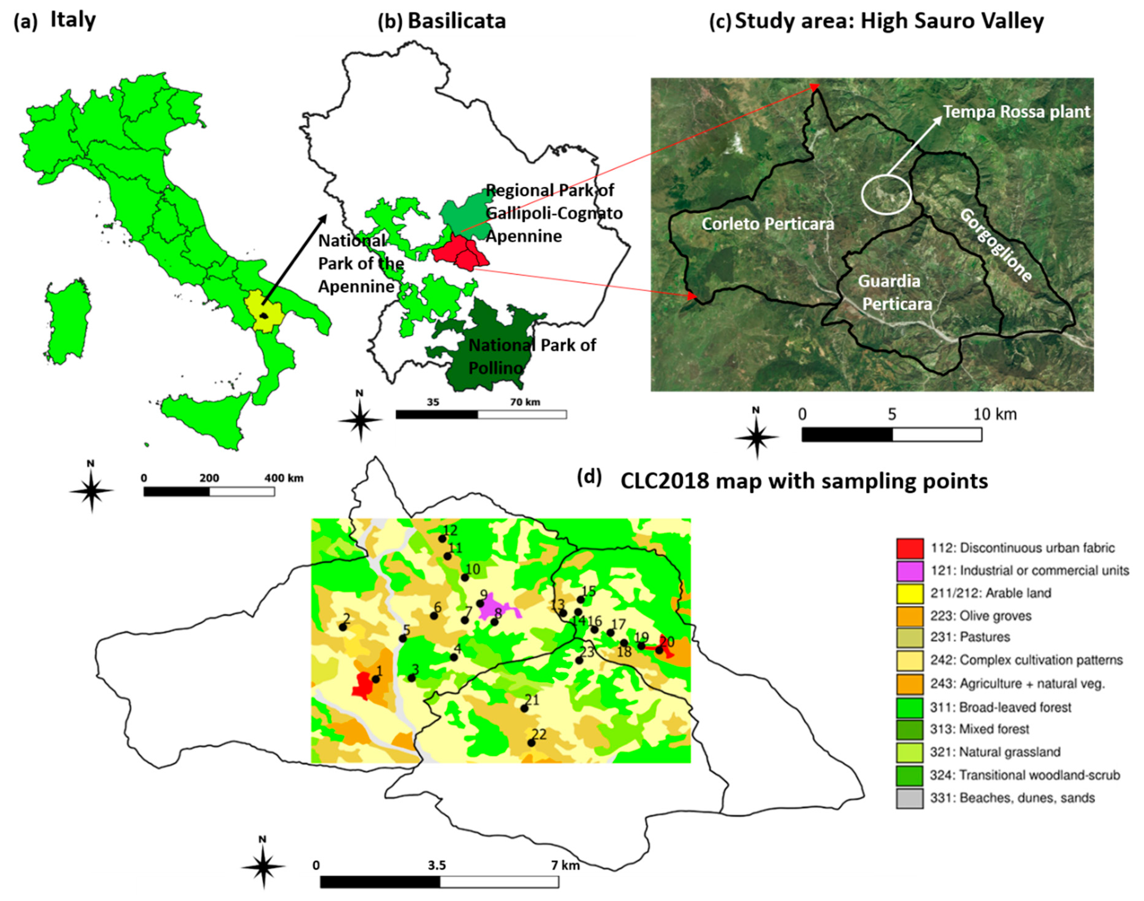
2.1. Site Description

The investigated area of the High Sauro Valley is in Basilicata (Southern Italy), one of the twenty administrative units (NUTS—Nomenclature of Territorial Units for Statistics) in which Italy is divided (Figure 1). The region has a large variety of landscapes with a dominant component of natural areas (forests, grasslands), often established as protected areas [35] in application of the European Habitats and Birds Directives (92/43/EC and 2009/147/EC). The High Sauro Valley, hosting the on-shore reservoir (crude oil and gas) and an oil/gas pre-treatment plant identified as “Tempa Rossa”, is located between the Gallipoli—Cognato Regional Park, the Appennino Lucano—Val d’Agri—Lagonegrese National Park and the Pollino National Park. The Tempa Rossa plant is in an area where natural and agricultural land covers are prevalent and the sealed areas are limited to the only urban centers of Gorgoglione, Corleto Perticara and Guardia Perticara, whose overall population is around 4000 inhabitants. When fully operational, the Tempa Rossa plant will be one of the most advanced plants, with a daily production capacity of approximately 50,000 barrels of oil, 230,000 m³ of natural gas, 240 tons of LPG (Liquefied Petroleum Gas) and 80 tons of sulfur (https://ep.totalenergies.com/en/projects/our-worldwide-presence/tempa-rossa-strategic-oil-field-economic-development-southern-italy, accessed on 30 June 2022). The climate of the study area is characteristic of the Mediterranean region. Winters can be very cold, while summers are moderately hot and dry, though night temperatures can be cool. The average values of the main meteorological parameters between October 2014 and November 2014 were temperature 13.79 °C, relative humidity 71%, atmospheric pressure 1176 hPa and wind speed 1.1 m/s, with SE and SW as prevailing directions. Weather measurements were provided by ALSIA (Lucana Agency for Development and Innovation in Agriculture, weather station of Guardia Perticara (https://www.alsia.it/opencms/opencms/Servizi/dettaglio/Accedi-ai-dati-agrometeorologici/, accessed on 30 June 2022)).

2.2. Bio-Monitors’ Sampling and Chemical Analysis

Samples of Evernia prunastri (L.) Ach. (Lichen fruticose species) were collected at an unpolluted site located in Rifreddo Forest (40°33′53.37″ N, 15°50′22.34″ E, about 1146 m a.s.l., Southern Italy) and prepared in the laboratory (i.e., dried at air to a constant weight and carefully cleaned to remove soil, bark and extraneous material). An aliquot of unexposed lichen collected in the control area was used to measure the pre-exposure trace element concentrations (ten replicas). About 3 g of dried material was used to prepare the lichen bags. The bags were exposed from October to November 2014 in 23 selected monitoring points covering an area of about 90 km² within the study area, where the Tempa Rossa plant is located approximately in the central position (Figure 1). At each site, two bags were hung on tree branches at a height of about 3 m above the ground. A Global Positioning System (GPS) was used for providing georeferenced on-site points. All samples after the exposition were stored in polyethylene bags until chemical analysis. Successively, 0.5 g dry weight (dw) of lichen samples were acidic-digested in a solution of 6 mL HNO₃ + 1 mL H₂O₂ [36] to determine the total concentration of 17 trace elements. In particular, the total concentrations of Al, Ca, Cr, Fe, Li, K, Mg, Mn, Na, P, S, Ti and Zn were measured by means of Inductively Coupled Plasma Optical Emission Spectrometry (ICP-OES), while Cd, Cu, Ni and Pb total concentrations were determined by Graphite Furnace Atomic Absorption Spectrometry (GF-AAS). The blank (reagent + beaker) contribution was for all the elements < 10% of the measured values. The method detection limit (MDL) was assessed. The validity of the whole analytical procedure was checked by using the International Atomic Energy Agency (IAEA) standard reference material, IAEA 336. The obtained values were in good agreement with the certified values (Table S1 in Supplementary Material).

2.3. Pollution Assessment

The contamination factor evaluates the degree of contamination for individual elements. The contamination factor (CF) was estimated as follows:

$$\mathrm{CF}=\mathrm{Cs}/\mathrm{Cb}$$

(1)

where Cs is the average concentration of each element in the exposed lichens and Cb is the average concentration of the same element at the background site. In this study, lichens previously collected at an unpolluted area in the Basilicata region in 2011 were chosen as the background [20].

The CFs values were classified into the following four classes: CF < 1.2 = no contamination (category C1), 1.2 ≤ CF < 2 = light contamination (category C2), 2 ≤ CF < 3 = medium contamination (category C3) and CF ≥ 3 = heavy contamination (category C4) [37].

The pollution load index (PLI) was also used to evaluate the overall air pollution load. PLI is defined as n- root of the product of the contamination factors for a given sample:

$$\mathrm{PLI}={\left({\mathrm{CF}}_1\times {\mathrm{CF}}_2\times {\mathrm{CF}}_3\times {\mathrm{CF}}_{4 }\times \dots {\mathrm{CF}}_{\mathrm{n}}\right)}^{1/\mathrm{n}}$$

(2)

where CF is a contamination factor and n is the number of studied elements. A PLI value less than 0.9 indicates an unpolluted area, a PLI approaching 1 (1 ± 0.1) indicates an air pollution load close to the background level and a value higher than 1 indicates low pollution (1.1 < PLI < 2.5), while very high pollution corresponds to PLI ≥ 2.5 [38,39].

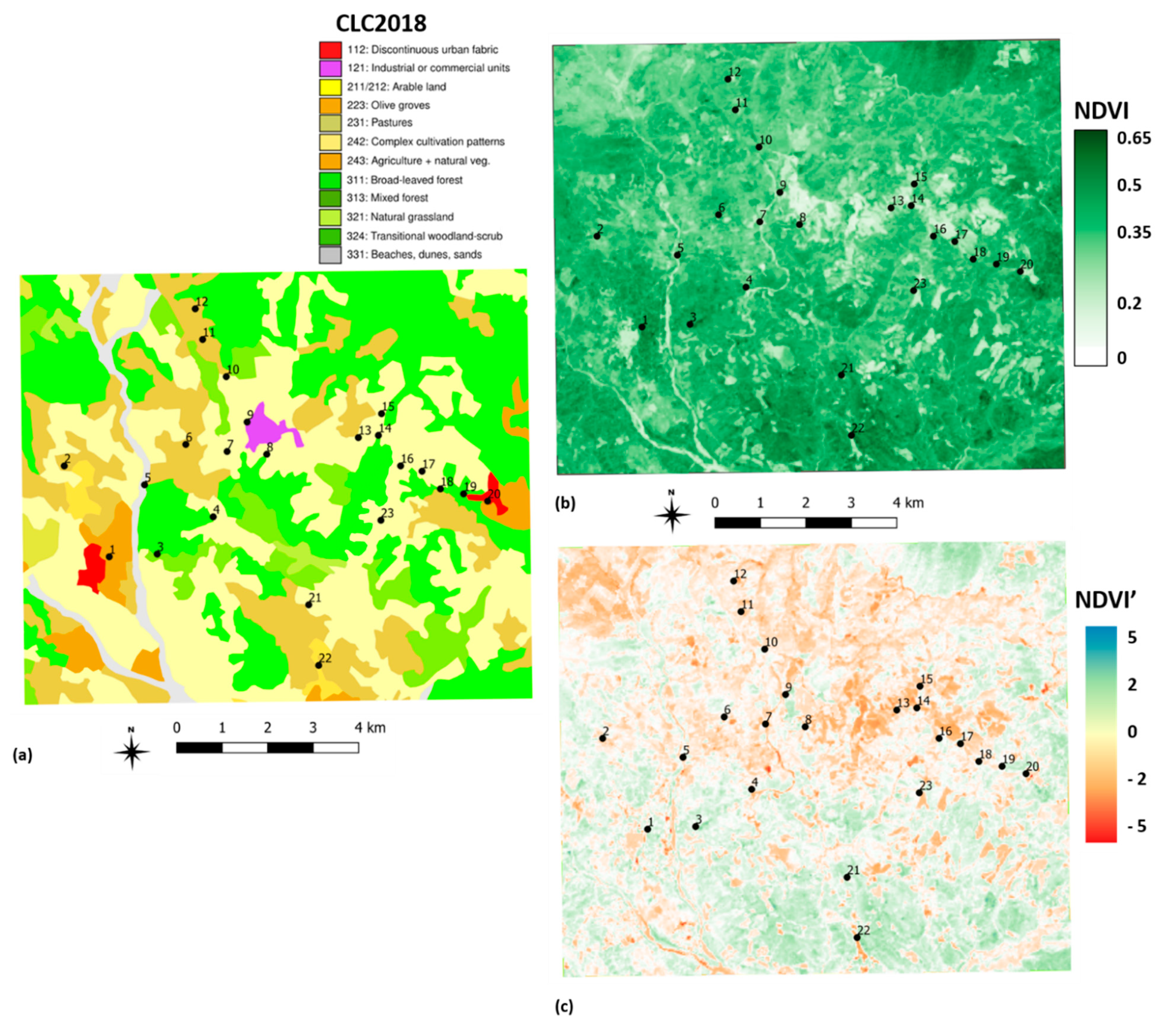
2.4. Land Cover and Satellite Observations

Multi-spectral satellite data with medium resolution are suitable to provide a quick snapshot of the vegetation conditions linked to plant vigor and biomass, chlorophyll and pigment contents. In this context, the historical Landsat archive enables us to go back in time. Since 1984, Landsat images have had a spatial resolution of 30 m with a time revisit of 16 days (Table S2 in Supplementary Material). Just one Landsat image was downloaded from the United States Geological Survey (USGS, https://earthexplorer.usgs.gov, accessed on 30 June 2022) as L2 level data (Land Surface Reflectance) and then clipped to the boundaries of the study area. In the investigated period, the available sensor was the OLI (Operational Land Imager) flying on Landsat 8. The image of the 30 November 2014 (188 path and 32 row GTCE) was selected based on cloud cover conditions (≈35% of the overall tile, but clouds occupied only zones outside the study area). To characterize photosynthetic levels and vegetation vigor of the different sampling points, the NDVI, i.e., the most adopted vegetation index, recognized as a suitable proxy for biomass content, phenological stage and vegetation vigor/health, was used [40,41,42].

It is calculated as follows:

$$\mathrm{NDVI}=\frac{{\mathsf{\rho }}_{\mathrm{nir}}-{\mathsf{\rho }}_{\mathrm{red}}}{{\mathsf{\rho }}_{\mathrm{nir}}+{\mathsf{\rho }}_{\mathrm{red}}}$$

(3)

where ρ_nir and ρ_red represent the near-infrared and red wavelengths of the electromagnetic spectrum corresponding, respectively, to the bands 5 and 4 of the OLI sensor.

NDVI values range from 0 to 1. High NDVI values are associated with healthy/dense vegetation, and medium–low NDVI values are common for stressed and/or sparse vegetation. Further lower values are associable to bare soils or partially sealed areas. To capture possible phenomena of anomalous levels of photosynthetic activity within the analyzed area, different vegetation layers characterizing the vicinity of the sampling points were considered by adopting the 2018 Corine Land Cover (CLC) map, which is a standard product of the Copernicus Program providing an inventory of 44 land cover classes at a European scale [43]. This way, the effects of biogeographic factors were removed from the calculation of this variable. Specifically, the procedure described in [44] was adopted. It consists in two essential steps:

• Estimation of mean values, μi(⋅), and standard deviation, σi(⋅), of NDVI for each CLC class type, with i = 1, …n, where n = number of different CLC classes characterizing the examined scene.
• Standardization of the NDVI distribution for each pixel of the given CLC class within the study area:

$${\mathrm{NDVI}}^{\prime }=\frac{\mathrm{NDVI}-\mathsf{\mu }\left(\mathrm{NDVI}\right)}{\mathsf{\sigma }\left(\mathrm{NDVI}\right)}$$

(4)

Standardization is finalized to allow the comparison among areas having different statistical distributions of the NDVI values. The resulting NDVI’ enables the detection of possible anomalies in photosynthetic activity that indicate areas with overt signs of vegetation stress. Integration, spatial analysis, and any calculations were carried out in GIS environment (QGIS 3.16.16, https://qgis.org/en/site/forusers/download.html, accessed on 30 June 2022) and the reference system used was the UTM projection (zone 33N).

2.5. Principal Component Analysis (PCA)

Principal component analysis (PCA) with varimax rotation was performed using the independent variables measured in 23 characteristic sampling points of the studied area to identify the main sources of atmospheric aerosol. Factor loading exceeding 0.7 was considered the most significant for each principal component. The factor loadings with eigenvalue >1 were kept, explaining 81.3% of the total variance. PCA resolved five principal components (PCs). The determined PC factor scores were used to evaluate observations with similar biomonitoring characteristics. PCA biplot (PC₁ vs. PC₂) was used to provide information about the relationship between monitoring points and variables in the studied area [45,46]. The statistical software used was R (R software) [47].

2.6. Human Health Risk Assessment

Risk assessment is an overall process or approach, used to identify health impacts and risk factors of exposure to a specific pollutant through different pathways [48]. The carcinogenic risk of exposure posed by Cd, Cr(VI), Ni and Pb through inhalation and the non-carcinogenic effect posed by Cd, Cr(VI), Cu, Mn, Ni, Pb and Zn through ingestion, dermal contact and inhalation pathways were evaluated using the model developed by the United States Environmental Protection Agency (US EPA, 2009 [49]). The carcinogenic and non-carcinogenic health risks were assessed for both children and adults, as reported in Section S1 in the Supplementary Material [50,51,52,53].

3. Results

3.1. ATEs Concentration and Air Pollution Assessment

The atmospheric trace element concentrations (ATEs) (i.e., Al, Ca, Cd, Cr, Cu, Fe, K, Li, Mg, Mn, Na, Ni, P, Pb, S, Ti and Zn) were assessed by means of “lichen-bag” monitors after 1-month exposure. Box-and-whisker plots depict the mean, median, 25th percentile (Q₁), 75th percentile (Q₃) and extreme values of the trace elements analyzed (Figure 2). The most abundant trace elements were Al, Ca, Fe, K, Mg and S, with mean concentrations above 1000 mg/kg. The next most abundant elements were Na, Mn and P, with mean concentrations between about 150 and 900 mg/kg. Zn, Pb and Ti showed a moderate abundance with concentrations above 20 mg/kg. The trace elements with concentrations less than 5 mg/kg were Cu, Cr, Li and Ni. Finally, Cd was the only trace element with concentration below 1 mg/kg (Table S3 in Supplementary Material).

The potential contamination level and risk linked to trace elements in the atmospheric aerosol was carried out using ecological indices. The analysis of the concentration of trace elements and the application of ecological indices may be considered as an important and useful method for evaluating the natural environment and the possible environmental hazards due to human impact. Therefore, the possible atmospheric contamination of each element in High Sauro Valley was assessed using two indices, the contamination factor (CF) and the pollution load index (PLI). The CF values used in this study differ slightly from the EC (exposed-to-control) ratio described by the authors of [54], who used the concentrations of trace elements in pre-exposed lichens as control values. In this study, lichens previously collected at an unpolluted area in the Basilicata region in 2011 [20] were chosen as background samples The CF values for each of the 17 trace elements analyzed range from 0.9 to 1.9. Particularly, the air pollution level of trace elements in the study area was estimated as not contaminated (C1) for Cr, Fe, Li, Mn, Ni, P, Pb S, Ti and Zn showing values <1.2 and slightly contaminated (C2) for the other trace elements such as Al, Ca, Cd, Cu, K, Na and Mg, that showed values ranging between 1.3 and 1.9 (Table S3 in Supplementary Material). The pollution load index (PLI) was assessed. A characteristic feature of this index is that it indicates mainly how many times the natural content of the studied metals was exceeded in the sampling site. Following the scale proposed by Tomlinson et al. [38], the results highlighted that 30% of the sampled points showed a PLI less than 0.9 or approaching 1 (1 ± 0.1), indicating no contamination or an air pollution load close to the background level. All the remaining points (70% of the total) showed values higher than 1 (ranging from 1.2 and 1.7, see Table S4 in Supplementary Material).

3.2. Satellite Observations

A non-invasive approach based on remote observations was adopted to assess the possible impact of anthropogenic activities on aerosol particles. In particular, the 30 November Landsat 8-OLI image, falling during the exposed period of the lichen bags, showed a limited variety of NDVI values. Looking at sampling points, most of them fall into pixels belonging to agricultural land uses (arable land and heterogeneous agricultural areas with the important presence of natural spaces, CLC classes 221 and 243 in Figure 3a) that usually have a low photosynthetic activity in the phenological stage examined (late Autumn).

All the samples exhibited medium–low NDVI values (ranging mainly from 0.3 to 0.45, see Figure 3b) that were also consistent with the prevalent mountainous character of the investigated landscapes [55]. Lastly, the NDVI’ (Figure 3c) showed a prevalence of low negative anomalies, pointing out a small deficit of the vegetation activity that usually characterizes the land cover classes investigated. Positive values are generally even less intense, meaning slightly better conditions in terms of photosynthetic activity than the average ones of the reference land cover class. Sampling points mostly fell in areas with low or very low negative values, indicating that vegetation conditions were generally not alarming. There were also some sampling points exhibiting very low positive values, meaning good vegetation conditions in these areas. The only criticalities were represented by the sampling points 7, 16 and 23, reaching values <−1.5, considered a statistically significant deviation from the mean conditions of the land cover classes to which these points belong (Table S4 in Supplementary Material, for further details see [44]). These sampling points fall in the 211 CLC land cover class (arable land) and are close to main and secondary roads.

3.3. Sources’ Identification

The principal component analysis (PCA) was performed by using the independent variables. Five PCAs with eigenvalues higher than 1.0 were taken out for the dataset of the whole sampling period, explaining 81.3% of the total variance. The Varimax rotation was used to clearly interpret the analytical results of the PCA. The PCA resolved five principal components (PCs) and their factor scores are plotted in Figure 4.

The first component (PC₁) explains about 24% of variance with high loading of Al, Fe, Li, Ti and K, mainly linked to geogenic origin such as crustal and rock erosion [56,57,58,59]. PC₁ also includes Cr. The origin of this last element should be linked both at vehicle exhausts, diesel vehicle engines and at geogenic nature [60,61,62]. The PC score of the first component shows a substantial spatial homogeneous distribution of the different elements included in this component, evidencing that sampling points with high PC₁ scores were characterized by the presence of crustal material or soil dust (Figure 4a). The second component (PC₂) with high loading of Cd, Ni, Pb, S and Zn explains about 22% of the variance and it is mainly attributable to anthropogenic sources identified as traffic [63,64]. As regards the spatial distribution of the score coefficients, relatively higher values were observed in the inner part of the investigated area characterized by the presence of construction sites and vehicle traffic, especially trucks (Figure 4b). K, Mg, Na and P show higher scores in the third component (PC₃), explaining about 15% of variance. As regards this component, the higher score seems located in the North-East of the investigated area (Figure 4c). This result could be due to punctual sources that can be found scattered in the study area. Particularly, K, Mg and P are generally linked to farming activities relating to mainly biomass combustion and post-harvest crop residue burned directly in the field [65,66]. Na could have a partial marine origin because the study area falls within the Mediterranean Basin. The fourth component with high loading of Ca, Mn and NDVI’ describes 13% of the total variance. Ca and Mn are likely related to the resuspension of local soil as well as road dust. PC₄ highlights a substantial score of spatial homogeneity with a slightly lower concentration located in the inner part of the study area (Figure 4d). In this area, the sampling points with low PC₄ scores are far from major roads, belonging mainly to arable lands and natural vegetation. Finally, the fifth component, explaining 8% of the total variance, includes only the Cu. Relatively higher scores were found towards the South direction (Figure 4e), probably due to the extensive management of permanent crops, as one of the major covers included in the heterogeneous agricultural areas (CLC classes 241, 242, 243), in which Cu was used [67].

3.4. Biplot PC₁ vs. PC₂

The PCA biplot displays both the loadings and the scores for the two selected main components (Figure 5). Looking at the biplot PC₁–PC₂, the configuration of the considered elements showed that there was a very large variance for the Pb, Zn, S, Ni, Fe and Cr and a somewhat large variance for Al and Ti. The variance was relatively small for the other elements. The vectors corresponding to the variables Pb and Zn as well as to the variables S and Ni were very close together, reflecting their relatively high positive correlation. The angle between the two vectors Pb and Zn and the other two vectors such as Ni and S is small, which indicated strong correlations between these elements. The vectors corresponding to the NDVI’ and S and Ni variables were very close, indicating a relatively positive correlation, justified by the nature of S and Ni which are essential nutrients for plants. In particular, S is considered a key macronutrient for plant growth and development [68], while a specific consideration is necessary for Ni. If it is available in moderate concentrations, it is a precious micronutrient, and a deficit of Ni can negatively interfere with vegetative growth processes [69], while high concentrations of Ni have been found to be toxic for plants [70]. Considering the simultaneous positions of the PC scores and loadings, the biplot diagram showed that the samples 1, 2, 9 and 22 were close to the direction of the Pb and Zn variables, suggesting, for the inner-product property, that the values of Pb and Zn were much higher than their average values.

Similarly, the relative positions of the samples 6, 8, 9 and 22, with respect to the variables S and Ni, indicated that the values of Ni and S were higher than their average values. The relative positions of the samples 22 and 9 with respect to the variable NDVI’ suggest that the NDVI’ value was higher than its average value. This is probably due to the size of the Landsat pixel (30 m), including in some cases a land use mix. Landsat pixels containing the samples 22 and 9 were labeled as partially sealed areas (falling within or near industrial and urban sites) but also including some natural areas that influence the overall value of the NDVI’. The samples 1, 2, 6 and 22 were close to industrial sites or little urban settlements. The samples 8 and 9 were near the large industrial site of Tempa Rossa, still under construction in the study period. The samples 22 and 9 share large values of Pb, Zn, S and Ni. The biplot also showed that samples 5, 14 and 21 were close to the opposite directions of the variables Pb and Zn. For these samples, the variables Pb and Zn were much lower than their average values. Moreover, the samples 4, 7, 12 and 18 were close and toward the opposite directions of the variables S and Ni. For these samples, the variables S and Ni are below their average values, especially for the samples 12 and 18. In particular, the sample 18 is in a heterogeneous agricultural area characterized by small anthropogenic covers (in this case a road), various agricultural uses and a considerable presence of natural vegetation (CLC class 243), whilst samples 5, 14 and 21 were representative of prevalently natural or agricultural areas very close to secondary roads. The samples 4 and 7 were positioned in rural areas and not so far from the industrial site of the Tempa Rossa plant. The samples 7 and 12 were oriented toward the opposite direction of the NDVI’ because of the negative values assumed by the variable in these points. More specifically, sample 7 was labeled as arable land (CLC class 211), but it is also characterized by low density of vegetation and by the presence of one of the busiest roads serving the industrial site. The sample 12 was located near an oil well, where low values of S and Ni, Pb, Zn and NDVI’ were recorded. The samples 11, 15 and 17 were close to the centroid. For these samples, the above-mentioned variables were close to their average values. The samples were located near some secondary roads with low traffic volume. The vectors corresponding to the variables Fe and Cr were very close, reflecting their large positive correlation. The vectors related to the variables Al and Ti were also comparatively close, indicating a positive correlation. The angle between the two vectors Fe and Cr and the other two, Al and Ti, was small, which indicates an overall positive correlation between these elements. The samples 6, 8, 9, 19 and 22 were close to the directions of Fe and Cr, implying that these variables are much higher than their average values. Likewise, the samples 6, 8 and 19 were positioned close to the directions of the Al and Ti variables, suggesting that they were much higher than their average values. These samples fall in urban/industrial land uses (small settlements, roads, industrial sites, etc.) where Fe, Cr, Al and Ti values were higher than their averages. The samples 4, 7, 12 and 18 were in the opposite direction of the variables Fe, Cr, Al and Ti. For these samples, especially 12 and 18, the variables Fe, Cr, Al and Ti showed values below their average values. The angle between the variables S, Ni and Fe, Cr was comparatively small, which indicates a positive correlation between these elements. Moreover, the angle between the variables S, Ni and Al, Ti was somewhat small, which also indicates a rather positive correlation between them. Peri-urban areas, little settlements and industrial construction sites with values of S and Ni higher than their averages can also have values of Fe and Cr higher than their averages. This was also observed for Al and Ti for the samples 6 and 8. Likewise, for sampling points located far from the industrial sites and roads and close to green areas, the variables S, Ni, Fe, Cr, Al and Ti exhibit values lower than their average values. The variables Pb and Zn are relatively orthogonal to the variables Al and Ti, and thus there is a very small correlation between Pb-Zn and Al-Ti. Therefore, two possible patterns were highlighted from the biplot: in the samples close to urban land uses, the variables Pb, Zn, S, Ni, Fe, Cr, Al and Ti were above their averages, while they were below their averages when samples were close to secondary roads or fell within green or agricultural areas. High values of NDVI’ are associated with high values of S and Ni, and to a lesser extent to Pb and Zn in urban and industrial samples.

4. Carcinogenic and Non-Carcinogenic Human Health Risk

According to the Integrated Risk Information Database (IRIS, https://www.epa.gov/iris, accessed on 30 June 2022) and the International Agency for Research on Cancer, many trace elements were classified as carcinogenic and non-carcinogenic. In this study, the trace elements Cd, Cr(VI), Ni and Pb were considered to be carcinogenic, while Cu, Mn and Zn were classified as non-carcinogenic. To have a whole environment framework of the study area, the potential human non-carcinogenic hazard (HQ) and excess lifetime cancer risk (ELCR), related to exposition of trace elements such as Cd, Cr(VI), Cu, Ni, Pb and Zn content in the atmospheric aerosol, were assessed for both children and adults (

Table 1. Non-carcinogenic trace elements’ health risk through inhalation (HQ_inh), ingestion (HQ_ing) and dermal exposure (HQ_derm), and the hazard index (HI) for both children and adults.

Elements	HQinh		HQing		HQderm
	Children	Adult	Children	Adult	Children	Adult
Cd	4.26 × 10−1	2.22 × 10−2	2.22 × 10−6	9.51 × 10−7	6.22 × 10−8	6.28 × 10−8
Cr(VI)	9.29 × 10−2	4.84 × 10−3	1.61 × 10−6	6.92 × 10−7	4.52 × 10−8	4.57 × 10−8
Cu	2.27 × 10−2	1.18 × 10−3	2.81 × 10−7	1.20 × 10−7	7.86 × 10−9	7.94 × 10−9
Ni	1.39	7.25 × 10−2	9.23 × 10−7	3.95 × 10−7	2.58 × 10−8	2.61 × 10−8
Pb	1.35 × 10−1	7.03 × 10−3	1.20 × 10−5	5.13 × 10−6	3.35 × 10−7	3.39 × 10−7
Zn	1.09 × 10−1	5.67 × 10−3	6.34 × 10−7	2.72 × 10−7	1.78 × 10−8	1.79 × 10−8
ΣHI	2.18	1.13 × 10−1	1.77x 10−5	7.57 × 10−6	4.94 × 10−7	4.99 × 10−7

).

Cd, Cr(VI), Cu, Ni, Pb and Zn non-carcinogenic trace elements’ health risk through inhalation (HQ_inh), ingestion (HQ_ing) and dermal exposure (HQ_derm), and the hazard index (HI), as the sum of the individual HQ_i, were considered. Cd, Pb and Zn presented HQ_inh values lower than the safe threshold (HQ = 1) both for children and adults, with values ranging between 1.09 × 10⁻¹ and 5.67 × 10⁻³. Therefore, the results showed no risk for inhalation, with the exception of Ni, which showed a value (1.39) just above the safe threshold for children through the inhalation pathway. The single HQ risks for the trace elements, considering the ingestion and dermal contact values, ranged between 7.75 × 10⁻⁶ and 1.77 × 10⁻⁵ and between 7.86 × 10⁻⁹ and 3.35 × 10⁻⁷, respectively. Therefore, no potential toxic health risks both for children and adults were evaluated through ingestion and dermal contact considering that the whole HQ_ing and HQ_derm values were below the safe threshold (HI < 1). Considering the cumulative health effect, only the HI_inh for the children showed a value of 2.18, above the safe threshold, indicating a possible non-carcinogenic risk from inhalation exposure mainly concerning Ni. The excess lifetime cancer risk (ELCR) and the integrated excess lifetime cancer risk (ΣELCR) were evaluated for Cd, Cr(VI), Ni and Pb (

Table 2. Excess lifetime cancer risk (ELCR) and the integrated excess lifetime cancer risk (ΣELCR) for both children and adults.

Elements	ELRC
	Children	Adult
Cd	3.43 × 10−8	1.37 × 10−7
Cr(VI)	3.49 × 10−6	1.40 × 10−5
Ni	2.09 × 10−7	8.35 × 10−7
Pb	4.31 × 10−9	1.73 × 10−8
ΣELRC	3.74 × 10−6	1.49 × 10−5

).

The ELRC cancer risk associated with the exposure to Cd, Cr(VI), Ni and Pb through the respiratory pathway for the local residents and for children was lower than the level of average risk acceptance of 10⁻⁶/year, indicating that the carcinogenic risk of these single trace elements is negligible. Considering the adults, ELCR for Cr(VI) indicated that the potential carcinogenic risk is not negligible [71,72]. Finally, concerning the integrated excess lifetime cancer risk (ΣELCR), it showed a value above the safe threshold for children, indicating no carcinogenic risk, and a value of 1.49 × 10⁻⁵ for adults, indicating that the carcinogenic risk mainly related to Cr(VI) is not negligible for the local adult population in the study area.

5. Discussion

The integrated holistic approach through biomonitoring techniques, NDVI and multivariate statistical analysis allowed to characterize the atmospheric aerosol particles in the studied area and the possible interactions between vegetation conditions and some pollutants of major interest.

To our knowledge, this study shows innovative aspects because it combines the consolidated practice of lichen-based biomonitoring and the equally robust, satellite-derived vegetation indices investigated through the adoption of a multivariate statistical analysis (PCA). As inferred from a large recent review on lichens as biological indicators [73], only few papers include the contextual use of lichen bio-monitors and vegetation indices (NDVI in particular), and only one adopts satellite data (specifically MODIS (Moderate-Resolution Imaging Spectroradiometer)) to derive NDVI estimates over a large area in China [74], with the other studies being based on spectroradiometer-derived NDVIs [75,76]. Furthermore, investigations conducted in remote areas, such as that presented in this paper, are rare [77], where most studies preferably focused on urban/industrial zones [73].

Concerning the adopted lichen species, we found that similar studies, relying on Evernia prunastri (L.) Ach, are rather frequent in Italy [78,79,80], where environmental monitoring policies have been recently strengthened by adding biomonitoring as one of the compulsory requirements for achieving environmental impact assessments [81].

Summarizing, considering the ecological indices applied to the whole area, there were no strong environmental criticalities with respect to the single element. However, considering all the elements analyzed together for a single sampling point, 70% of them showed a low-pollution condition.

In agreement with the feature of the investigated area, the studies showed that natural crustal resuspension, vehicle traffic, especially trucks, farming activities relating to biomass combustion and post-harvest crop residue burned directly in the field and extensive management of permanent crops represented the main potential sources of atmospheric aerosol particles in the High Sauro Valley.

Concerning Pb, Zn, S, Ni, Fe, Cr, Al and Ti, a non-homogeneous distribution of these trace elements was pointed out. Close to urban sites, little settlements, industrial sites and roads, they were found above their averages, mainly due to the traffic and crustal sources. Close to vegetation and agricultural areas with a scarce presence of anthropogenic covers (mainly secondary roads), Pb, Zn, S, Ni, Fe, Cr, Al and Ti were below their averages. These findings may be due to different scattered sources of the trace elements, and they were confirmed by NDVI’ remote observations, indicating only sporadic cases of moderate extent concerning photosynthetic activity anomalies, generally ascribable to the size of the Landsat pixel, including, in some cases, more than one land cover (CLC class). Furthermore, associations between S, Ni, Pb, Zn and NDVI’ were highlighted, indicating a possible positive interaction between low concentrations of some air pollutants and vegetation conditions.

Considering the NDVI’, high values were associated with high values of S and Ni, and to a lesser extent to Pb and Zn, in urban and industrial samples, indicating a possible beneficial interaction between the observed low concentrations of these elements and vegetation conditions. In fact, Ni and Zn are considered micro-nutrients for plant life when available in moderate amounts [69,82]. In our investigations, all the elements did not show high concentration values, confirming the beneficial link between Ni-Zn and vegetation. This was also true for S, which, as highlighted above, represents a macronutrient for plants. Lastly, the presence of Pb, notoriously considered as toxic and mostly linked to traffic and industrial emissions, does not seem to have had a significant impact on vegetation conditions, probably due to its moderate concentration.

Finally, regarding the health risk impact of atmospheric trace elements on the exposed population, both children and adults, considering inhalation, ingestion and the dermal contact pathway, the studies highlighted a possible non-carcinogenic risk concerning Ni and a not-negligible carcinogenic risk related to Cr(VI) for the adult population in the study area.

6. Conclusions

The main objective of this study was to characterize the atmospheric aerosol particles by assessing the trace element concentrations, identifying their sources and assessing the possible interaction with vegetation conditions. To this aim, a holistic integrated approach through biomonitoring techniques, NDVI’ and multivariate statistical analysis was adopted in a semi-rural area (High Sauro Valley—Southern Italy) before the on-shore reservoir and the related oil/gas pre-treatment plant were fully operative. The ecological indices evaluated for the seventeen atmospheric trace elements (Al, Ca, Cd, Cr, Cu, Fe, K, Li, Mg, Mn, Na, Ni, P, Pb, S, Ti and Zn) pointed out an overall low air pollution load. Principal component analysis identified both natural and anthropogenic trace element sources, such as crustal resuspension, soil and road dust, traffic, biomass burning and agricultural practices. Moreover, the PC score maps pointed out a non-homogeneous distribution of the trace elements analyzed. The biplot highlighted that the variables Pb, Zn, S, Ni, Fe, Cr, Al and Ti, close to urban sites, little settlements, industrial sites and roads, were above their averages, mainly due to the traffic and crustal sources. Concerning the sampling points close to vegetation and agricultural areas with a scarce presence of anthropogenic covers (mainly secondary roads), the variables Pb, Zn, S, Ni, Fe, Cr, Al and Ti were below their averages. The health risk impact of atmospheric trace elements on the exposed population of both children and adults highlighted a possible non-carcinogenic risk concerning Ni and a not-negligible carcinogenic risk related to Cr(VI) for the adult population in the study area. This work provides a low-cost and effective procedure for monitoring atmospheric air quality, also considering the possible interaction between the impact of anthropogenic activities and health vegetation conditions. In particular, the proposed approach can be useful in making environmental assessments of air quality, vegetation and human health of those prevalently rural areas where a conversion to urban/industrial/commercial land uses has been planned, with possible impacts on air quality, on the stock of natural capital and thus on the ability of the local ecosystems to efficiently provide goods and services.

References

1. Liu, Y.; You, S.; Li, N.; Fang, J.; Jia, J.; Li, X.; Ren, J. Study on the Agricultural Air Pollution Aggravated by the Rural Labor Migration. Atmosphere 2022, 13, 174. [Google Scholar] [CrossRef]
2. Bodor, K.; Szép, R.; Bodor, Z. Time Series Analysis of the Air Pollution around Ploiesti Oil Refining Complex, One of the Most Polluted Regions in Romania. Sci. Rep. 2022, 12, 11817. [Google Scholar] [CrossRef] [PubMed]
3. Caggiano, R.; Sabia, S.; Speranza, A. Trace Elements and Human Health Risks Assessment of Finer Aerosol Atmospheric Particles (PM1). Environ. Sci. Pollut. Res. 2019, 26, 36423–36433. [Google Scholar] [CrossRef]
4. Hien, T.T.; Chi, N.D.T.; Huy, D.H.; Le, H.A.; Oram, D.E.; Forster, G.L.; Mills, G.P.; Baker, A.R. Soluble Trace Metals Associated with Atmospheric Fine Particulate Matter in the Two Most Populous Cities in Vietnam. Atmos. Environ. X 2022, 15, 100178. [Google Scholar] [CrossRef]
5. Kim, K.-H.; Kabir, E.; Kabir, S. A Review on the Human Health Impact of Airborne Particulate Matter. Environ. Int. 2015, 74, 136–143. [Google Scholar] [CrossRef]
6. Gautam, S.; Kumar, P.; Patra, A.K. Occupational Exposure to Particulate Matter in Three Indian Opencast Mines. Air Qual. Atmos. Health 2016, 9, 143–158. [Google Scholar] [CrossRef]
7. Bunch, A.G.; Perry, C.S.; Abraham, L.; Wikoff, D.S.; Tachovsky, J.A.; Hixon, J.G.; Urban, J.D.; Harris, M.A.; Haws, L.C. Evaluation of Impact of Shale Gas Operations in the Barnett Shale Region on Volatile Organic Compounds in Air and Potential Human Health Risks. Sci. Total Environ. 2014, 468–469, 832–842. [Google Scholar] [CrossRef]
8. Ramirez, M.I.; Arevalo, A.P.; Sotomayor, S.; Bailon-Moscoso, N. Contamination by Oil Crude Extraction—Refinement and Their Effects on Human Health. Environ. Pollut. 2017, 231, 415–425. [Google Scholar] [CrossRef]
9. Hussain, I.; Puschenreiter, M.; Gerhard, S.; Sani, S.G.A.S.; Khan, W.; Reichenauer, T.G. Differentiation between Physical and Chemical Effects of Oil Presence in Freshly Spiked Soil during Rhizoremediation Trial. Environ. Sci. Pollut. Res. 2019, 26, 18451–18464. [Google Scholar] [CrossRef]
10. Johnston, J.E.; Lim, E.; Roh, H. Impact of Upstream Oil Extraction and Environmental Public Health: A Review of the Evidence. Sci. Total Environ. 2019, 657, 187–199. [Google Scholar] [CrossRef]
11. Besser, H.; Hamed, Y. Causes and Risk Evaluation of Oil and Brine Contamination in the Lower Cretaceous Continental Intercalaire Aquifer in the Kebili Region of Southern Tunisia Using Chemical Fingerprinting Techniques. Environ. Pollut. 2019, 253, 412–423. [Google Scholar] [CrossRef] [PubMed]
12. Sahebari, M.; Ayati, R.; Mirzaei, H.; Sahebkar, A.; Hejazi, S.; Saghafi, M.; Saadati, N.; Ferns, G.A.; Ghayour-Mobarhan, M. Serum Trace Element Concentrations in Rheumatoid Arthritis. Biol. Trace Elem. Res. 2016, 171, 237–245. [Google Scholar] [CrossRef] [PubMed]
13. Nunes, F.L.d.S.; Lima, S.C.V.C.; Lyra, C.d.O.; Marchioni, D.M.; Pedrosa, L.F.C.; Barbosa Junior, F.; Sena-Evangelista, K.C.M. The Impact of Essential and Toxic Elements on Cardiometabolic Risk Factors in Adults and Older People. J. Trace Elem. Med. Biol. 2022, 72, 126991. [Google Scholar] [CrossRef] [PubMed]
14. Lukaski, H.C.; Klevay, L.M.; Milne, D.B. Effects of Dietary Copper on Human Autonomic Cardiovascular Function. Europ. J. Appl. Physiol. 1988, 58, 74–80. [Google Scholar] [CrossRef]
15. Martin, S.; Griswold, W. Human Health Effects of Heavy Metals. Environ. Sci. Technol. Brief. Cit. 2009, 15, 1–6. [Google Scholar]
16. Zeng, X.; Xu, C.; Xu, X.; Zhang, Y.; Huang, Y.; Huo, X. Elevated Lead Levels in Relation to Low Serum Neuropeptide Y and Adverse Behavioral Effects in Preschool Children with E-Waste Exposure. Chemosphere 2021, 269, 129380. [Google Scholar] [CrossRef]
17. Rodriguez, J.H.; Weller, S.B.; Wannaz, E.D.; Klumpp, A.; Pignata, M.L. Air Quality Biomonitoring in Agricultural Areas Nearby to Urban and Industrial Emission Sources in Córdoba Province, Argentina, Employing the Bioindicator Tillandsia Capillaris. Ecol. Indic. 2011, 11, 1673–1680. [Google Scholar] [CrossRef]
18. Malaspina, P.; Casale, M.; Malegori, C.; Hooshyari, M.; Di Carro, M.; Magi, E.; Giordani, P. Combining Spectroscopic Techniques and Chemometrics for the Interpretation of Lichen Biomonitoring of Air Pollution. Chemosphere 2018, 198, 417–424. [Google Scholar] [CrossRef]
19. Kardel, F.; Wuyts, K.; De Wael, K.; Samson, R. Biomonitoring of Atmospheric Particulate Pollution via Chemical Composition and Magnetic Properties of Roadside Tree Leaves. Environ. Sci. Pollut. Res. 2018, 25, 25994–26004. [Google Scholar] [CrossRef]
20. Caggiano, R.; Calamita, G.; Sabia, S.; Trippetta, S. Biomonitoring of Atmospheric Pollution: A Novel Approach for the Evaluation of Natural and Anthropogenic Contribution to Atmospheric Aerosol Particles. Environ. Sci. Pollut. Res. 2017, 24, 8578–8587. [Google Scholar] [CrossRef]
21. Caggiano, R.; Trippetta, S.; Sabia, S. Assessment of Atmospheric Trace Element Concentrations by Lichen-Bag near an Oil/Gas Pre-Treatment Plant in the Agri Valley (Southern Italy). Nat. Hazards Earth Syst. Sci. 2015, 15, 325–333. [Google Scholar] [CrossRef] [Green Version]
22. Cucu-Man, S.-M.; Steinnes, E. Analysis of Selected Biomonitors to Evaluate the Suitability for Their Complementary Use in Monitoring Trace Element Atmospheric Deposition. Environ. Monit. Assess 2013, 185, 7775–7791. [Google Scholar] [CrossRef] [PubMed]
23. Samela, C.; Imbrenda, V.; Coluzzi, R.; Pace, L.; Simoniello, T.; Lanfredi, M. Multi-Decadal Assessment of Soil Loss in a Mediterranean Region Characterized by Contrasting Local Climates. Land 2022, 11, 1010. [Google Scholar] [CrossRef]
24. De Fioravante, P.; Luti, T.; Cavalli, A.; Giuliani, C.; Dichicco, P.; Marchetti, M.; Chirici, G.; Congedo, L.; Munafo, M. Multispectral Sentinel-2 and SAR Sentinel-1 Integration for Automatic Land Cover Classification. Land 2021, 10, 611. [Google Scholar] [CrossRef]
25. Pflugmacher, D.; Rabe, A.; Peters, M.; Hostert, P. Mapping Pan-European Land Cover Using Landsat Spectral-Temporal Metrics and the European LUCAS Survey. Remote Sens. Environ. 2019, 221, 583–595. [Google Scholar] [CrossRef]
26. D’Emilio, M.; Coluzzi, R.; Macchiato, M.; Imbrenda, V.; Ragosta, M.; Sabia, S.; Simoniello, T. Satellite Data and Soil Magnetic Susceptibility Measurements for Heavy Metals Monitoring: Findings from Agri Valley (Southern Italy). Environ. Earth Sci. 2018, 77, 63. [Google Scholar] [CrossRef]
27. Zhang, H.; Lan, Y.; Lacey, R.; Hoffmann, W.C.; Huang, Y. Analysis of Vegetation Indices Derived from Aerial Multispectral and Ground Hyperspectral Data. Int. J. Agric. Biol. Eng. 2009, 2, 33–40. [Google Scholar] [CrossRef]
28. Strong, C.J.; Burnside, N.G.; Llewellyn, D. The Potential of Small-Unmanned Aircraft Systems for the Rapid Detection of Threatened Unimproved Grassland Communities Using an Enhanced Normalized Difference Vegetation Index. PLoS ONE 2017, 12, e0186193. [Google Scholar] [CrossRef]
29. Buitink, J.; Swank, A.M.; van der Ploeg, M.; Smith, N.E.; Benninga, H.-J.F.; van der Bolt, F.; Carranza, C.D.U.; Koren, G.; van der Velde, R.; Teuling, A.J. Anatomy of the 2018 Agricultural Drought in the Netherlands Using in Situ Soil Moisture and Satellite Vegetation Indices. Hydrol. Earth Syst. Sci. 2020, 24, 6021–6031. [Google Scholar] [CrossRef]
30. Jiang, X.; Zhen, J.; Miao, J.; Zhao, D.; Shen, Z.; Jiang, J.; Gao, C.; Wu, G.; Wang, J. Newly-Developed Three-Band Hyperspectral Vegetation Index for Estimating Leaf Relative Chlorophyll Content of Mangrove under Different Severities of Pest and Disease. Ecol. Indic. 2022, 140, 108978. [Google Scholar] [CrossRef]
31. Bedair, R.; Ibrahim, A.A.; Alyamani, A.A.; Aloufi, S.; Ramadan, S. Impacts of Anthropogenic Disturbance on Vegetation Dynamics: A Case Study of Wadi Hagul, Eastern Desert, Egypt. Plants 2021, 10, 1906. [Google Scholar] [CrossRef] [PubMed]
32. Conti, M.E.; Iacobucci, M.; Cucina, D.; Mecozzi, M. Multivariate Statistical Methods Applied to Biomonitoring Studies. Int. J. Environ. Pollut. 2007, 29, 333–343. [Google Scholar] [CrossRef]
33. Agnan, Y.; Probst, A.; Séjalon-Delmas, N. Evaluation of Lichen Species Resistance to Atmospheric Metal Pollution by Coupling Diversity and Bioaccumulation Approaches: A New Bioindication Scale for French Forested Areas. Ecol. Indic. 2017, 72, 99–110. [Google Scholar] [CrossRef]
34. Hussain, S.; Hoque, R.R. Biomonitoring of Metallic Air Pollutants in Unique Habitations of the Brahmaputra Valley Using Moss Species—Atrichum Angustatum: Spatiotemporal Deposition Patterns and Sources. Environ. Sci. Pollut. Res. 2022, 29, 10617–10634. [Google Scholar] [CrossRef] [PubMed]
35. Imbrenda, V.; Lanfredi, M.; Coluzzi, R.; Simoniello, T. A Smart Procedure for Assessing the Health Status of Terrestrial Habitats in Protected Areas: The Case of the Natura 2000 Ecological Network in Basilicata (Southern Italy). Remote Sens. 2022, 14, 2699. [Google Scholar] [CrossRef]
36. Loppi, S.; Frati, L. Lichen Diversity and Lichen Transplants as Monitors of Air Pollution in a Rural Area of Central Italy. Environ. Monit. Assess 2006, 114, 361–375. [Google Scholar] [CrossRef]
37. Boamponsem, L.K.; Adam, J.I.; Dampare, S.B.; Nyarko, B.J.B.; Essumang, D.K. Assessment of Atmospheric Heavy Metal Deposition in the Tarkwa Gold Mining Area of Ghana Using Epiphytic Lichens. Nucl. Instrum. Methods Phys. Res. Sect. B Beam Interact. Mater. At. 2010, 268, 1492–1501. [Google Scholar] [CrossRef]
38. Tomlinson, D.L.; Wilson, J.G.; Harris, C.R.; Jeffrey, D.W. Problems in the Assessment of Heavy-Metal Levels in Estuaries and the Formation of a Pollution Index. Helgol. Meeresunters 1980, 33, 566–575. [Google Scholar] [CrossRef]
39. Salo, H.; Bućko, M.S.; Vaahtovuo, E.; Limo, J.; Mäkinen, J.; Pesonen, L.J. Biomonitoring of Air Pollution in SW Finland by Magnetic and Chemical Measurements of Moss Bags and Lichens. J. Geochem. Explor. 2012, 115, 69–81. [Google Scholar] [CrossRef]
40. Coluzzi, R.; Fascetti, S.; Imbrenda, V.; Italiano, S.S.P.; Ripullone, F.; Lanfredi, M. Exploring the Use of Sentinel-2 Data to Monitor Heterogeneous Effects of Contextual Drought and Heatwaves on Mediterranean Forests. Land 2020, 9, 325. [Google Scholar] [CrossRef]
41. Coluzzi, R.; D’Emilio, M.; Imbrenda, V.; Giorgio, G.A.; Lanfredi, M.; Macchiato, M.; Ragosta, M.; Simoniello, T.; Telesca, V. Investigating Climate Variability and Long-Term Vegetation Activity across Heterogeneous Basilicata Agroecosystems. Geomat. Nat. Hazards Risk 2019, 10, 168–180. [Google Scholar] [CrossRef] [Green Version]
42. Greco, S.; Infusino, M.; De Donato, C.; Coluzzi, R.; Imbrenda, V.; Lanfredi, M.; Simoniello, T.; Scalercio, S. Late Spring Frost in Mediterranean Beech Forests: Extended Crown Dieback and Short-Term Effects on Moth Communities. Forests 2018, 9, 388. [Google Scholar] [CrossRef]
43. Büttner, G.; Kosztra, B.; Soukup, T.; Sousa, A.; Langanke, T. CLC2018 Technical Guidelines; European Environment Agency: Copenhagen, Denmark, 2017. [Google Scholar]
44. Lanfredi, M.; Coppola, R.; Simoniello, T.; Coluzzi, R.; D’Emilio, M.; Imbrenda, V.; Macchiato, M. Early Identification of Land Degradation Hotspots in Complex Bio-Geographic Regions. Remote Sens. 2015, 7, 8154–8179. [Google Scholar] [CrossRef]
45. Gabriel, K.R. The Biplot Graphic Display of Matrices with Application to Principal Component Analysis. Biometrika 1971, 58, 453–467. [Google Scholar] [CrossRef]
46. Jolliffe, I.T. Principal Component Analysis; Springer: Cambridge, UK, 2002; pp. 29–61. ISBN 978-0-387-22440-4. [Google Scholar]
47. Kahle, D.; Wickham, H. Ggmap: Spatial Visualization with Ggplot2. R J. 2013, 5, 144. [Google Scholar] [CrossRef]
48. Zhao, S.; Yu, Y.; Xia, D.; Yin, D.; He, J.; Liu, N.; Li, F. Urban Particle Size Distributions during Two Contrasting Dust Events Originating from Taklimakan and Gobi Deserts. Environ. Pollut. 2015, 207, 107–122. [Google Scholar] [CrossRef] [PubMed]
49. US EPA. U.S. Environmental Protection Agency; Sacks, J. Integrated Science Assessment (ISA) for Particulate Matter (Final Report, December 2009). Available online: https://cfpub.epa.gov/ncea/risk/recordisplay.cfm?deid=216546 (accessed on 19 July 2022).
50. Hu, X.; Zhang, Y.; Ding, Z.; Wang, T.; Lian, H.; Sun, Y.; Wu, J. Bioaccessibility and Health Risk of Arsenic and Heavy Metals (Cd, Co, Cr, Cu, Ni, Pb, Zn and Mn) in TSP and PM2.5 in Nanjing, China. Atmos. Environ. 2012, 57, 146–152. [Google Scholar] [CrossRef]
51. US EPA. Risk Assessment Guidance for Superfund (RAGS): Part A. Available online: https://www.epa.gov/risk/risk-assessment-guidance-superfund-rags-part (accessed on 21 July 2022).
52. Wang, X.; Bi, X.; Sheng, G.; Fu, J. Chemical Composition and Sources of PM10 and PM2.5 Aerosols in Guangzhou, China. Environ. Monit. Assess 2006, 119, 425–439. [Google Scholar] [CrossRef]
53. US EPA. Regional Screening Levels (RSLs)—Generic Tables. Available online: https://www.epa.gov/risk/regional-screening-levels-rsls-generic-tables (accessed on 21 July 2022).
54. Frati, L.; Brunialti, G.; Loppi, S. Problems Related to Lichen Transplants to Monitor Trace Element Deposition in Repeated Surveys: A Case Study from Central Italy. J. Atmos. Chem. 2005, 52, 221–230. [Google Scholar] [CrossRef]
55. Quaranta, G.; Salvia, R.; Salvati, L.; Paola, V.D.; Coluzzi, R.; Imbrenda, V.; Simoniello, T. Long-Term Impacts of Grazing Management on Land Degradation in a Rural Community of Southern Italy: Depopulation Matters. Land Degrad. Dev. 2020, 31, 2379–2394. [Google Scholar] [CrossRef]
56. Khillare, P.S.; Balachandran, S.; Meena, B.R. Spatial and Temporal Variation of Heavy Metals in Atmospheric Aerosol of Delhi. Environ. Monit. Assess 2004, 90, 1–21. [Google Scholar] [CrossRef]
57. Begum, B.A.; Biswas, S.K.; Hopke, P.K. Key Issues in Controlling Air Pollutants in Dhaka, Bangladesh. Atmos. Environ. 2011, 45, 7705–7713. [Google Scholar] [CrossRef]
58. Begum, B.A.; Hossain, A.; Saroar, G.; Biswas, S.K.; Nasiruddin, M.; Nahar, N.; Chowdury, Z.; Hopke, P.K. Sources of Carbonaceous Materials in the Airborne Particulate Matter of Dhaka. Asian J. Atmos. Environ. 2011, 5, 237–246. [Google Scholar] [CrossRef]
59. Jain, S.; Sharma, S.K.; Mandal, T.K.; Saxena, M. Source Apportionment of PM10 in Delhi, India Using PCA/APCS, UNMIX and PMF. Particuology 2018, 37, 107–118. [Google Scholar] [CrossRef]
60. Chandra Mouli, P.; Venkata Mohan, S.; Balaram, V.; Praveen Kumar, M.; Jayarama Reddy, S. A Study on Trace Elemental Composition of Atmospheric Aerosols at a Semi-Arid Urban Site Using ICP-MS Technique. Atmos. Environ. 2006, 40, 136–146. [Google Scholar] [CrossRef]
61. Wang, Y.-F.; Huang, K.-L.; Li, C.-T.; Mi, H.-H.; Luo, J.-H.; Tsai, P.-J. Emissions of Fuel Metals Content from a Diesel Vehicle Engine. Atmos. Environ. 2003, 37, 4637–4643. [Google Scholar] [CrossRef]
62. Lilli, M.A.; Moraetis, D.; Nikolaidis, N.P.; Karatzas, G.P.; Kalogerakis, N. Characterization and Mobility of Geogenic Chromium in Soils and River Bed Sediments of Asopos Basin. J. Hazard. Mater. 2015, 281, 12–19. [Google Scholar] [CrossRef]
63. Gupta, A.K.; Karar, K.; Srivastava, A. Chemical Mass Balance Source Apportionment of PM10 and TSP in Residential and Industrial Sites of an Urban Region of Kolkata, India. J. Hazard. Mater. 2007, 142, 279–287. [Google Scholar] [CrossRef]
64. Chelani, A.B.; Gajghate, D.G.; Devotta, S. Source Apportionment of PM10 in Mumbai, India Using CMB Model. Bull Environ. Contam. Toxicol. 2008, 81, 190–195. [Google Scholar] [CrossRef]
65. Andreae, M.O.; Merlet, P. Emission of Trace Gases and Aerosols from Biomass Burning. Glob. Biogeochem. Cycles 2001, 15, 955–966. [Google Scholar] [CrossRef]
66. Akagi, S.K.; Yokelson, R.J.; Wiedinmyer, C.; Alvarado, M.J.; Reid, J.S.; Karl, T.; Crounse, J.D.; Wennberg, P.O. Emission Factors for Open and Domestic Biomass Burning for Use in Atmospheric Models. Atmos. Chem. Phys. 2011, 11, 4039–4072. [Google Scholar] [CrossRef] [Green Version]
67. Ballabio, C.; Panagos, P.; Lugato, E.; Huang, J.-H.; Orgiazzi, A.; Jones, A.; Fernández-Ugalde, O.; Borrelli, P.; Montanarella, L. Copper Distribution in European Topsoils: An Assessment Based on LUCAS Soil Survey. Sci. Total Environ. 2018, 636, 282–298. [Google Scholar] [CrossRef] [PubMed]
68. Li, Q.; Gao, Y.; Yang, A. Sulfur Homeostasis in Plants. Int. J. Mol. Sci. 2020, 21, 8926. [Google Scholar] [CrossRef] [PubMed]
69. Bai, C.; Reilly, C.C.; Wood, B.W. Nickel Deficiency Disrupts Metabolism of Ureides, Amino Acids, and Organic Acids of Young Pecan Foliage. Plant Physiol. 2006, 140, 433–443. [Google Scholar] [CrossRef] [PubMed]
70. Rooney, C.P.; Zhao, F.-J.; McGrath, S.P. Phytotoxicity of Nickel in a Range of European Soils: Influence of Soil Properties, Ni Solubility and Speciation. Environ. Pollut. 2007, 145, 596–605. [Google Scholar] [CrossRef]
71. Sánchez-Soberón, F.; Rovira, J.; Mari, M.; Sierra, J.; Nadal, M.; Domingo, J.L.; Schuhmacher, M. Main Components and Human Health Risks Assessment of PM10, PM2.5, and PM1 in Two Areas Influenced by Cement Plants. Atmos. Environ. 2015, 120, 109–116. [Google Scholar] [CrossRef]
72. Hieu, N.T.; Lee, B.-K. Characteristics of Particulate Matter and Metals in the Ambient Air from a Residential Area in the Largest Industrial City in Korea. Atmos. Res. 2010, 98, 526–537. [Google Scholar] [CrossRef]
73. Abas, A. A Systematic Review on Biomonitoring Using Lichen as the Biological Indicator: A Decade of Practices, Progress and Challenges. Ecol. Indic. 2021, 121, 107197. [Google Scholar] [CrossRef]
74. Huang, R.; Ju, T.; Dong, H.; Duan, J.; Fan, J.; Liang, Z.; Geng, T. Analysis of Atmospheric SO2 in Sichuan-Chongqing Region Based on OMI Data. Environ. Monit. Assess 2021, 193, 849. [Google Scholar] [CrossRef]
75. Garty, J.; Kloog, N.; Cohen, Y.; Wolfson, R.; Karnieli, A. The Effect of Air Pollution on the Integrity of Chlorophyll, Spectral Reflectance Response, and on Concentrations of Nickel, Vanadium, and Sulfur in the LichenRamalina Duriaei (De Not.) Bagl. Environ. Res. 1997, 74, 174–187. [Google Scholar] [CrossRef]
76. Garty, J.; Weissman, L.; Cohen, Y.; Karnieli, A.; Orlovsky, L. Transplanted Lichens in and around the Mount Carmel National Park and the Haifa Bay Industrial Region in Israel: Physiological and Chemical Responses. Environ. Res. 2001, 85, 159–176. [Google Scholar] [CrossRef] [Green Version]
77. Incerti, G.; Cecconi, E.; Capozzi, F.; Adamo, P.; Bargagli, R.; Benesperi, R.; Carniel, F.C.; Cristofolini, F.; Giordano, S.; Puntillo, D.; et al. Infraspecific Variability in Baseline Element Composition of the Epiphytic Lichen Pseudevernia Furfuracea in Remote Areas: Implications for Biomonitoring of Air Pollution. Environ. Sci. Pollut. Res. 2017, 24, 8004–8016. [Google Scholar] [CrossRef] [PubMed]
78. Nannoni, F.; Santolini, R.; Protano, G. Heavy Element Accumulation in Evernia Prunastri Lichen Transplants around a Municipal Solid Waste Landfill in Central Italy. Waste Manag. 2015, 43, 353–362. [Google Scholar] [CrossRef] [PubMed]
79. Loppi, S.; Paoli, L. Comparison of the Trace Element Content in Transplants of the Lichen Evernia Prunastri and in Bulk Atmospheric Deposition: A Case Study from a Low Polluted Environment (C Italy). Biologia 2015, 70, 460–466. [Google Scholar] [CrossRef]
80. Vannini, A.; Paoli, L.; Nicolardi, V.; Di Lella, L.A.; Loppi, S. Seasonal Variations in Intracellular Trace Element Content and Physiological Parameters in the Lichen Evernia Prunastri Transplanted to an Urban Environment. Acta Bot. Croat. 2017, 76, 171–176. [Google Scholar] [CrossRef]
81. Cioffi, M. Air quality monitoring with the lichen biodiversity index (lbi) in the district of Faenza (Italy). EQA Int. J. Environ. Qual. 2009, 1, 1–6. [Google Scholar] [CrossRef]
82. Sharma, A.; Patni, B.; Shankhdhar, D.; Shankhdhar, S.C. Zin—An Indispensable Micronutrient. Physiol. Mol. Biol. Plants 2013, 19, 11–20. [Google Scholar] [CrossRef]
Figure 1. The High Sauro Valley (c) located in Basilicata (b), a region of Southern Italy (a), that includes, among others, the municipalities of Gorgoglione, Guardia Perticara and Corleto Perticara, where the Tempa Rossa plant has been built. (d) The Corine Land Cover 2018 (CLC2018) was used as the main map to identify the different land covers of the investigated area, falling prevalently within the three mentioned municipalities. The numbers 1–23 represent the sampling points.
Atmosphere 13 01501 g001
Figure 2. Boxplot shows the concentrations observed after a 1-month exposure of each considered element. Horizontal lines show the median values, while the point indicates the mean value.
Atmosphere 13 01501 g002
Figure 3. (a) CLC2018, (b) NDVI values and (c) NDVI’ values. All the maps show the sampling points overlapped. The numbers 1–23 represent the sampling points.
Atmosphere 13 01501 g003
Figure 4. Maps of the PC_score plot with respect to the observations of the five components extracted (ae). The numbers 1–23 represent the sampling points.
Atmosphere 13 01501 g004
Figure 5. Biplot PC1 vs. PC2, arrows indicate variables and numbers indicate observations. The numbers 1–23 represent the sampling points.
Atmosphere 13 01501 g005