Extreme Value Analysis and Modelling of Wet Snow Accretion on Overhead Lines in Hungary

Abstract

Wet snow events in Hungary can occasionally cause damage to overhead power lines and serious power supply failures. Return period calculation of such high snow mass events was determined upon a 50-year long data series available at 12 meteorological stations. Wet snow masses were estimated with a model of cylindrical accretion around wire of 3.1 cm diameter. Trends in the return periods and ice classes (according to the ISO 12494 standard) were assessed from division of the dataset into two periods (1965–1990 and 1991–2016). Ice classes in the range of R2 to R5 (mass of 0.7–6.1 kg m⁻¹) were identified. The wet snow risk decreased in southern or central Hungary, while an increase was found in the western part of Hungary. Ice classes R6–R8 (up to 40 kg m⁻¹) could occur in mountain areas of Hungary as indicated by numerical simulations in case studies. However, their return period is unknown due to the lack of long observation series.

1. Introduction

Wet snow occurs at both middle and higher latitudes, as an annual phenomenon. On exposed objects, especially on overhead power lines, cylindrical accumulation of snow can be significant and can cause extensive damage to transmission line networks. For decades, diversified scientific examinations have been conducted to study the appearance and formation [1,2,3,4,5], the possibility and reliability of its prediction [6,7,8,9] and to develop prevention methods [10,11,12]. The formation of wet snow crystals needs special atmospheric conditions. The dry snowflakes, while falling pass through a layer with a slightly positive temperature, partially melt, so liquid water (optimally 10–15%) appears among the crystal branches. Due to the liquid water content, snowflakes can strongly adhere to objects reaching critical masses for damages. In the accumulation phase, the height of the 0 °C isotherm, the moisture content of both the air and the snowflakes, furthermore the wind conditions experienced during snowfall hold decisive importance. Based on the study of Somfalvi-Tóth [13] the optimal vertical stratification for wet snow formation is a 300–400 m thick, slightly positive (maximum + 2 °C) layer near the ground under a negative temperature layer, which is also demonstrated by a narrow interval of lapse rate (3–4 °C km⁻¹). The 850/1000 hPa relative topography also moves in a narrow range (1292–1307 gpm) during wet snow events. The relative humidity of the air is mostly between 90–95%. Besides these components, wind speed is also an important factor. If the wind speed is initially weak (below 5 m s⁻¹), the accumulation starts at the top of the transmission lines, almost perpendicular to its longitudinal axis. If the wind speed does not exceed 5 m s⁻¹, the rotation of the wire around its axis is not able to start due to the weak compressive force of the wind ($\overrightarrow{F_{wind}})$. If the wind speed exceeds 5 m s⁻¹, the snowflakes accumulate on the wire at the spatial angle of their collision [14]. If there are irregular peaks in the pressure of the wind (e.g., turbulence), which is accompanied by an insufficiently high adhesion force ($\overrightarrow{F_a)}$ between the wire and the snow layer, the accumulated snow sleeve may collapse from the overhead line.

Measurements of the accumulated wet snow mass require specific equipments and measuring devices (e.g., to consider the rotation of wire and obtain cylindrical accretion in windy situations) and are typically installed at observatories and sites with frequent occurrence of this phenomenon [15,16]. Sometimes, direct measurements are provided from samples of snow accreted on damaged overhead power lines. Such information is usually sparse and can occur at a site, where measurements of other meteorological parameters are not available. Thus, even in case of major wet snow-related damage, wet snow mass or other meteorological parameters can be sometimes only estimated upon photographs, results of accretion models, numerical analyses and forecasts [3].

In Hungary, occurrence of wet snow was registered from 1966 to 2014 at meteorological stations using icing measurement rods (ice metres). However, it was usually considered that it only rarely causes major damage to the high-voltage electric power lines and it was only marginally mentioned in meteorological publications [17]. The first severe wet snow event, which was studied in detail, using station measurements and numerical models, appeared in southwestern Hungary on 27–28 January 2009 [7]. Other events accompanied with damages were reported also in later years, in 2013 and 2016 [9,18]. Direct measurements were available only for a few situations, indicating that in case of damaged overhead lines at least 4–5 kg m⁻¹ of snow was accreted [19].

An extreme event with high precipitation (up to 80 mm in 48 h measured at certain stations) and wet snow accumulation on electric power lines occurred on 19–20 April 2017, mainly in the mountain region in the North of Hungary and close to the capital of Hungary—Budapest (Figure 1a,b).

Another example of an event constrained mainly to hilly or mountain area was reported on 12–13 April 2021 in northwestern Hungary.

Current research of wet snow extremes in Hungary has been evolving along two branches (Figure 2). The first one was a climatological examination of wet snow including the frequency of occurrence, the maximum accretion of wet snow on wires (kg m⁻¹) based on the observations of basic meteorological parameters of 12 synoptic stations possessing 50-year long dataset. Furthermore, the 50-year and 100-year return periods of wet snow accretion on overhead transmission lines was estimated. It was the first study of this kind in Hungary and its aim was to specify extreme mass values and ice categories possibly occurring at the examined sites and to identify tendencies of wet snow severity during the recent years/decades. The second branch concerned Numerical Weather Prediction (NWP) simulations with the ALADIN model (Aire Limitée Adaptation Dynamique Développement InterNational) [20,21]. NWP outputs provided us with further information about the magnitude of snow mass accumulation in severe wet snow events as the return period calculation only marginally described conditions in mountain terrain of Hungary. Thus, the two above-mentioned cases from the years 2017 and 2021 are presented here in more detail.

As NWP forecasts exhibit both systematic and random errors, the magnitude of the model forecast error of wet snow mass was estimated. There was no direct information from field measurements, hence the reference data were obtained from wet snow parameterization and station measurements of variables (2 m temperature, 10 m wind speed, precipitation) provided on input. Impact of other factors on the mass calculation (e.g., correction of precipitation undercatch, wet snow density estimation) was also studied.

This paper is divided into six main sections. The next Section (number 2) is devoted to data and methods and it is divided into four subsections. The Section 2.1. presents the input station observations, their locations and metadata. The Section 2.2. explains the method of wet snow parameterization, which was common for both return period calculation and NWP simulation. The Section 2.3. describes the method of extreme value analysis and return period calculation. Section 2.4. gives overview of the Numerical Weather Prediction (NWP) models utilized and some details about the model forecast error analysis (Figure 2).

Section 3 and Section 4 present results of the 50-year and 100-year return period calculation and show the two wet snow cases with more details on spatial distribution of mass in mountain regions of Hungary (Figure 2).

Discussion of results, impacts and uncertainties in the wet snow mass and return period calculation can be found in Section 5. Conclusions are given in Section 6.

2. Materials and Methods

2.1. Input Data for Calculating the 50- and 100-Year Return Periods of Wet Snow Mass

We used 50 years of data from 12 meteorological stations in Hungary to study the return periods of wet snow events. We selected stations, where visual observations were available from 1 January 1965 to 31 December 2016. These stations are Békéscsaba, Budapest-Pestszentlőrinc, Debrecen, Győr, Miskolc, Pápa, Pécs, Siófok, Szeged, Szolnok, Szombathely (

Table 1. Metadata of meteorological stations in Hungary. Height above the sea level (a.s.l) is displayed in meters.

Station Name	Label	Latitude	Longitude	Height a.s.l. [m]
Békéscsaba	1	46.7	21.1	89
Budapest-Pestszentlőrinc	2	47.4	19.3	139
Debrecen	3	47.5	21.6	121
Győr	4	47.6	17.6	108
Kékestető	5	47.9	20.0	1012
Miskolc	6	48.1	20.7	162
Pápa	7	47.3	17.4	200
Pécs	8	46.0	18.2	153
Siófok	9	46.9	18.1	124
Szeged	10	46.2	20.1	76
Szolnok	11	47.1	20.2	68
Szombathely	12	47.2	16.6	209

).

In the case of Kékestető, the existence of the entire 50-year data series was not available, because regular observations began in 1966. The latter calculations were not affected by this 1-year lack of data, because a 20-year data series is sufficient to calculate the 50-year return period [22,23].

The data for extreme value analysis were obtained from the database of the Hungarian Meteorological Service (OMSZ). The selection criteria for defining wet snow conditions were as follows:

• The temperature at 2 m was between −0.5 and +2 °C;
• Snowfall was recorded at the time of observation (synoptic code: 70, 71, 72, 73, 74, 75);
• End of the event: if the temperature rose above +2 °C and/or precipitation ceased and no precipitation was registered for 6 h thereafter.

The needed and selected variables for calculations were 2 m temperature (°C), precipitation amount (mm) and wind speed and hourly wind gust (m s⁻¹). The data were substituted into Equations (1)–(9). in order to calculate the estimated wet snow mass (kg m⁻¹) on the transmission lines.

The automatic weather stations (AWS) used for the case studies differed from the locations in the previous examination (most of the selected stations can be found in mountain areas or near mountains). These stations are provided by OMSZ as well but in contrast to the stations mentioned in Table 1, they do not contain information about the precipitation type. The list of the main metadata of AWSs can be seen in

Table 2. List of AWS stations used for case studies and their a.s.l. height in meters. The A10 station (Budapest Zugliget) is not depicted on maps due to its close proximity to Budapest János-hegy (1.3 km distance).

Label (Figure 3)	Station	Station Height (m)	NWP Model Height
			ALADIN/ SHMU	ALADIN/ HS1A
A1	Budapest János-hegy	516	394	446
A2	Eger	225	214	202
A3	Miskolc Szentlélek	752	724	754
A4	Nagy Hideg hegy	855	568	793
A5	Gerecse tető	620	373	584
A6	Kab-hegy	595	485	525
A7	Sümeg	195	174	176
A8	Tés	472	464	467
A9	Sülysáp	181	159	190
A10	Budapest Zugliget	421	394	405

. The geographical locations of all weather stations are displayed in Figure 3. The A10 station (Budapest Zugliget) was not depicted on maps due to its close proximity to Budapest János-hegy (A1) (1.3 km distance).

Visual observations were presented with 3 h temporal resolution at the synoptic stations until 1995/1996, but after the installation of the automatic weather stations, hourly measurements have been available. Nikolov and Makkonen [25] examined several wet snow calculation methods and came to the conclusion that the method also used in this study [26] is not sensitive to the choice of time step to an extent that would significantly modify the results.

2.2. Parameterization of Wet Snow Accretion

The basic equations and physical processes related to all types of atmospheric icing are described in ISO 12424 [22]. However, several methods have been developed to model the properties of wet snow, e.g., snow density, diameter of the sleeve on wires, additional extra masses and forces along transmission lines [3,26,27,28]. The method we used was described by Admirat [26]. The following equation describes the connection between the diameter of the snow cylinder appearing on the overhead line and its mass M (kg):

$$\Phi \frac{d\Phi }{dt}=\frac{2}{{\varrho }_{snow}\pi }\frac{dM}{dt}$$

(1)

where Φ (m) is the diameter, while ρ_snow (kg·m⁻³) is the density of the accumulating snow. The change of the mass over time is proportional to the flux R (m³·s⁻¹) of the snow passing through the unit surface S (m²). If we assume that the flow is perpendicular to this surface, then

$$R=c \sqrt{u^2+w^2 }S$$

(2)

where c is the mass concentration of snowflakes in the air (kg·m⁻³), u (m·s⁻¹) is the horizontal component of the wind, w (m·s⁻¹) is the terminal velocity of snow crystals. In practice, the mass concentration of snowflakes is not measured, so a parameterization is required:

$$c=\frac{P}{3600w}$$

(3)

where P (mm h⁻¹) is the intensity of precipitation and w = 1.5 m·s⁻¹ are the terminal velocity of wet snowflakes [16]. The change of mass over time can be written as follows:

$$\frac{dM}{dt}=\beta R=\frac{\beta P}{3600}\sqrt{1+\frac{u^2}{w^2}}\Phi$$

(4)

where β is the so-called sticking efficiency, which defines the ratio of the density flux of sticking out of the hitting snow particles per unit area of the overhead lines. According to Nygaard et al. [29], the parameterization of sticking efficiency is the following:

$$\beta =\frac{1}{\sqrt{u}}$$

(5)

So the sticking efficiency of snowflakes is inversely proportional to the square root of the horizontal wind component (u). The stronger the wind, the less efficiently the snowflakes adhere to the wire. If the wind speed is below 1 m·s⁻¹, then β can be considered 1. The change of the diameter of the wet snow sleeve over time [26] is

$$\frac{d\varphi }{dt}=\frac{2K}{{\rho }_{snow}\pi }$$

(6)

$$where K=\frac{\beta kP}{3600}\sqrt{1+\frac{u^2}{w^2}}$$

(7)

where the new factor of k in Equation (7) is the correction factor of precipitation amount measured in a Hellmann precipitation gauge during snowfall. The higher the wind speed, the higher the rate of missed snowflakes is due to the turbulent flow developing around the top of the gauge, so the catch ratio (CR) will be less than 1 [30]. The CR can be calculated by the following formula:

CR = 96.63 + 0.41 U’² − 9.84U’ + 5.95 T_a

(8)

where U’ is the wind speed measured at the height of the precipitation gauge. That is 70% of the wind speed (m s⁻¹) measured at a height of 10 m [31], T_a is the air temperature (°C). CR is a percentage value, so the correction factor k of the precipitation amount P in Equation (7) can be written as:

k = 100/CR

(9)

In the case of modelling of wet snow accretion by using Numerical Weather Prediction (NWP) models, the value of k can be considered 1.

The snow density (ρ_snow) varies between 100 and 800 kg·m⁻³ [26]. However, Wakahama et al. [1] showed that the density of accumulated snow also depends on the intensity of precipitation, in our calculations the constant density value of 300 kg m⁻³ was used. According to studies by Deneau and Guillot [32], the density of the accreted snow cylinder varies between 300–500 kg·m⁻³ in cases when the wind velocity does not exceed 8 m·s⁻¹. In Hungary, the average wind speed during wet snow events does not exceed 5 m·s⁻¹ in 75% of the cases. The rate of wind speed over 10 m·s⁻¹ is approximately 1% [13]. Therefore, in our study the calculations were performed by using the lower limit of snow density (300 kg·m⁻³), because it is inversely proportional to the accreted snow mass (Equation (6)), so the lower the snow density, the higher the estimated snow mass on the wires which approach covers the aim of the study, i.e., the description of climatically possible extremes of wet snow events.

Selection of critical constants: an important step during the calculations both in extreme value analysis and modelling by NWPs is the parameterization of the sticking efficiency (β). For this, we examined the accumulation of wet snow calculated with the 4 parameterization methods most often recommended in the literature [28,29,33,34]. The best estimation was achieved by Nygaard et al. [29] (Equation (5)) based on the work of Somfalvi-Tóth [13], so this method was used also in this study, but the results of the extreme value analysis with all of the listed methods can be found in Somfalvi-Tóth [13] in detail.

In addition, the density of the accumulated snow cylinder is also an important issue. ISO 12424 [22] suggests 300 kg·m⁻³ and 500 kg·m⁻³. Now, the results are presented here based on the density of 300 kg·m⁻³ (suggested for low or moderate wind speed), but all calculations were also performed with 4 density values (200 kg·m⁻³, 300 kg·m⁻³ and 400 kg·m⁻³, 200 + 20 × U kg·m⁻³ (U wind speed (m·s⁻¹), [26]) in Somfalvi-Tóth [13].

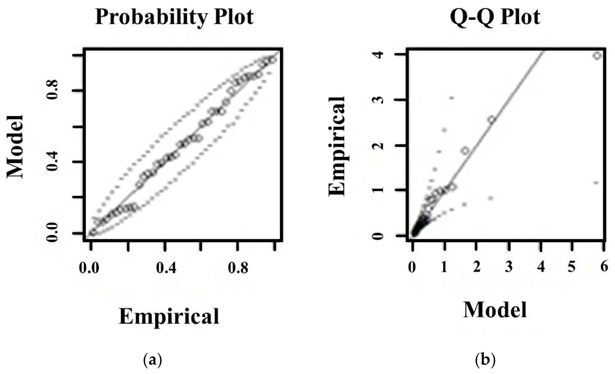
2.3. Extreme Value Analysis with the Peaks over Threshold Method

The temporal distribution of wet snow appearance is irregular, i.e., the occurrence of the phenomenon may accumulate in certain years, which may be followed with no formation of wet snow for several years [23]. These wet snow occurrences appear in the data series as random outliers, so-called peaks with higher values among the mainly data of zeros. An extreme value test, the Peaks Over Threshold (POT) method is the most suitable for the statistical analysis of a phenomena with behavior like this [35,36]. The POT method is for estimating the distribution of extremes above a well-chosen threshold value. The purpose of extreme value analysis is to examine the probability of events that are outside the scope of the observed data. The statistical analysis is based on the generalized extreme value distribution, which can be used on datasets with sufficiently large numbers of cases with minimum 20-year long observations [23]. The advantage of the POT method is that all the data are involved into the determination of the threshold value.

Pareto distribution: The accurate determination of this threshold is important. The well-determined threshold ensures that the distribution of the exceeding data follow the generalized Pareto distribution [37]. So the distribution function of generalized Pareto distribution can be written as the following:

$$H\left(y\right)=1-{\left(1+\frac{\xi y}{\sigma }\right)}^{-\frac{1}{\xi }}, ha \xi \ne 0,$$

(10)

where y > 0 and 1 + ξy/σ > 0. The σ means the scale parameter, ξ is the shape parameter. The location parameter (µ = 0 in this case) defines the center of the distribution, the scale parameter (σ) determines the size of the deviation around the location parameter µ, while the shape parameter (ξ) influences the behavior of the tales of the distribution function. The values of the shape parameter ξ and the scale parameter σ must be estimated in the POT method. The log-likelihood estimation gives the best parameter estimation in the extreme value calculations of wet snow (Nygaard et al. 2014). We suppose that n random variables exceed the threshold x_i = Y_i − u, Y_i > u, i = 1, …., n. Then, according to Matyasovszky and Lakatos [38] the log-likelihood function is the following:

If ξ ≠ 0,

$$l\left(\sigma ,\xi \right)=-k log\sigma -\left(1+\frac{1}{\xi }\right){\displaystyle \sum }_{i=1}^{n}log\left(1+\frac{{\xi }_i}{\sigma }\right).$$

(11)

If ξ = 0,

$$l\left(\sigma \right)=-k log\sigma -{\sigma }^{-1}{\displaystyle \sum }_{i=1}^n{x}_i$$

(12)

Then, Equation (11) or Equation (12) must be maximized according to ($\sigma ,\xi )$ Selection of the threshold: a key step during the calculations is the selection of the thresholds. The threshold value should not be too high, because then there will not be a sufficient number of samples to perform the calculations and the variance will be large. If, on the other hand, the threshold is low and too much data is involved into the calculation, then the bias will be increased. The optimal threshold must be chosen by considering these limiting factors [38]. Two different methods were applied in our study to calculate the thresholds, the so-called Mean Residual Life Plot (MRL plot) [37] and the Dispersion Index Plot [39]. Both methods are identically able to estimate the threshold, however both of the methods were used to ensure the appropriate determination of thresholds. During the calculations, 24 threshold values were estimated for the 12 weather stations and for the 2 periods (1965–1990 and 1991–2016).

The MRL method is based on the estimation of the expected values of the wet snow mass (kg m⁻¹) with Pareto distribution. Let Y₁, Y₂,...,Y_n be independent, identically distributed random variables that exceed the threshold value u₀ and follow the generalized Pareto distribution with the shape parameter ξ and the scale parameter σ. [37]. Then, the expected value can be determined as follows:

$$E\left(Y\right)=\frac{\sigma }{1-\xi }, ha \xi <1$$

(13)

If the wet snow mass values (kg·m⁻¹) above the u₀ threshold follow the Pareto distribution, then all the threshold above this u₀ threshold will fulfill this condition. So the lowest threshold must be chosen for the best estimation [37] (Figure 4a).

The other threshold selection method was the Dispersion Index Plot method, which can be considered as a control next to the previous one. In this case, the parameters of the generalized Pareto distribution and their stability are estimated and examined [39]. Let Y₁, Y₂,...,Y_n be independent random variables with a generalized Pareto distribution,and with the parameters of shape parameter ξ₀, scale parameter σ₀, and location parameter µ₀. Let u be a threshold for which u > u₀ is true. If we randomly select a variable Y_k|Y_n > u, then the following relationships can be written

$${\sigma }_u={\sigma }_0+{\xi }_0\left(u-u_0\right)$$

(14)

$${\xi }_u={\xi }_0$$

(15)

$${\sigma }^{*}={\sigma }_u-{\xi }_{u}u$$

(16)

If u₀ is a suitable threshold, then σ* and ξ_u will be constants for all u > u₀, so the asymptotic stability of the scale and shape parameters ensures constancy while u₀ is changing [39]. In practice, this means that above the optimal threshold the values of the estimated parameters will become constants (Figure 4b).

Goodness of fit test was achieved to prove the existence of the Pareto distribution on values above the estimated threshold. To achieve this goal, two widely used graphical methods were applied, the so-called Probability Plot and the Q-Q Plot.

Probability Plot: Let Y₁, Y₂,...,Y_n, arranged in ascending order, be independent, identically distributed random variables that exceed the threshold value u₀. In the case of a sufficiently good estimation, the value of the relative frequency {i/(n + 1); i = 1,…,n} and the value of the estimated parameters {H(Y(i)); i = 1,…,n} fall close to each other, so depicted on a graph they fluctuate around a line in an XY diagram (Figure 5a). This is called a Probability Plot [38].

Q-Q Plot: The other approach is the quantile diagram, where—if the fitted distribution is good—the quantiles of the estimated (model) and real (empirical) values also fall close to each other, so these values also fluctuate around a straight line. This is called a quantile-quantile or Q-Q Plot diagram (Figure 5b). The dashed lines in both plots indicates the 95% confidence intervals.

Calculation of the return periods and return values: The ultimate goal of extreme value analysis is to perform a risk assessment of the probability of occurrence of very rare events, and to calculate the possible maximum (minimum) values for a given period (10, 20, 50, 100 years). In our work we calculated the 50- and 100-year return values of the wet snow mass (kg·m⁻¹) accreted as an extra mass on overhead lines according to the recommendations of the ISO 12494 (2001) standard document.

Let Y₁, Y₂,...,Y_n be independent, identically distributed random variables that follow the generalized Pareto distribution with the parameters of ξ shape parameter and σ scale parameter. Let u denote the appropriately chosen threshold value. Then, the conditional probability of a given variable can be given as follows:

$$P\left(Y>u\right)={\left(1+\xi \left(\frac{y-u}{\sigma }\right)\right)}^{-\frac{1}{\xi }}$$

(17)

which is rearranging according to the rules of the conditional probability is the following:

$$P\left(Y>y\right)=P\left(Y>u\right){\left(1+\xi \left(\frac{y-u}{\sigma }\right)\right)}^{-\frac{1}{\xi }}$$

(18)

If it is supposed that the random variable Y_m occurs only once out of every m observations, then it can be written that

$$P\left(Y_m>u\right){\left(1+\xi \left(\frac{y-u}{\sigma }\right)\right)}^{-\frac{1}{\xi }}=\frac{1}{m}$$

(19)

Equation (19). converted gives the Y_m return value of the mth detection:

$$Y_m=u+\frac{\sigma }{\xi }\left({\left(m{p}_u\right)}^{\xi }-1\right), if \xi \ne 0$$

(20)

$$Y_m=u\sigma loglog \left(m{p}_u\right) , if \xi =0$$

(21)

where p_u = P (Y > u).

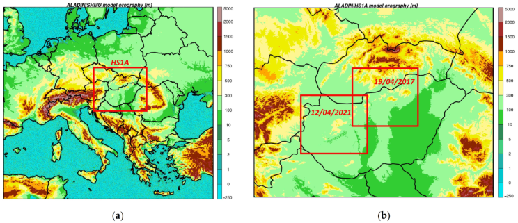
2.4. Description of the Numerical Weather Prediction Models and Analysis of Forecast Accuracy

For the discussion of the applicability of results of return period calculation in mountain terrain (Section 4 and Section 5), the ALARO canonical configuration of the ALADIN model [40] was run to simulate severe wet snow cases. ALADIN is a limited area NWP model, which provides analyses and short-range weather forecasts of various prognostic and diagnostic meteorological parameters [41].

Two versions of the ALADIN model were run for the study, denoted ALADIN/SHMU and ALADIN/HS1A. ALADIN/SHMU [42,43] is a hydrostatic model with 4.5 km horizontal resolution grid and an own assimilation cycle for local surface observations of temperature and humidity including the CANARI interpolation [44] (

Table 3. Main characteristics of the ALADIN model configurations used for the wet snow case studies.

Model Version	ALADIN/SHMU	ALADIN/HS1A
Status	operational	experimental
Horizontal resolution	4.5 km	1.0 km
Number of vertical levels	63	73
Domain size	2813 × 2592 km	720 × 576 km
Coupling model	ARPEGE, 3 h coupling frequency	ALADIN/SHMU, 3 h coupling frequency
Initialization	none	none
Data assimilation	optimal interpolation CANARI [44]	none (dynamical and LBC downscaling)
Dynamics	hydrostatic, spectral, semi-implicit, 2 time level semi-lagrangian scheme	non-hydrostatic, spectral, semi-implicit 2 time level iterative lefted implicit scheme
Physics	ALARO-1vB	ALARO-1vB, adapted for convection-permitting scales (after [57,58])

). The lateral boundary conditions were obtained from the forecasts of the global model ARPEGE [45,46] run at Météo-France. The dynamics of the model is based on spectral, semi-implicit, 2 time-level semi-lagrangian scheme [47,48].

ALADIN/HS1A was run as a downscaling of the ALADIN/SHMU model to a 1 km resolution grid applying a 2-time-level iterative centered implicit scheme [49] for its dynamics. HS1A provided finer orography in the mountainous regions of Hungary (Figure 6a,b), where wet snow-related damages were reported in the years 2017 and 2021.

Both ALADIN/SHMU and ALADIN/HS1A used nearly the same setup of physical parameterization denoted ALARO-1vB, including the emulated Turbulent Kinetic Energy (TKE) -based scheme [50,51], parameterization of deep convection [52] and microphysics [53] adapted for the mesoscale. Surface processes were parameterized with the ISBA (Interaction Soil Biosphere Atmosphere) scheme [54] utilizing the 1 km resolution ECOCLIMAP I and ECOCLIMAP II databases [55,56] for physiographic data.

The physical parameterization and postprocessing of ALADIN/SHMU and ALADIN/HS1A provides also calculation of parameters of wet snow and ice accretion on overhead wires based on the above-mentioned Admirat [26] method and its Equations (1)–(7). In both cases (based on 19 April 2017 00 UTC and on 12 April 2021 00 UTC), 48 h forecasts of wet snow mass were carried out with the same criterions for wet snow and the same accretion technique as in the return period calculations presented in this paper (see Section 2.1 and 2.2). The precipitation phase (rain/snow) was inferred from the ALADIN/ALARO parameterization of microphysics and precipitation fluxes [53]. Parameterization of snow shedding and thawing was not implemented, thus the outputs represent the maximum possible wet snow mass in the respective situation.

Estimation of the model forecast error of wet snow mass was done at locations with available measurements from AWS and synoptic stations. The reference wet snow mass (kg·m⁻¹) was parameterized upon the same criterions and approaches as for return period calculations (see Section 2.1 and 2.2), using temperature, wind speed and total precipitation (rain + snow) from station observations with 1 h frequency. Since precipitation type was not observed at AWS stations, the fraction of rain/snow was derived from calculations of the ALADIN/SHMU and ALADIN/HS1A models. The algorithm selected a grid-point from an area of 9 × 9 grid-points near the position of stations, where the model height was closest to station one. Model parameters referred then to this grid-point. At the Budapest Zugliget station only temperature measurements were available, wind and precipitation was derived from model forecasts.

The input wet snow precipitation was corrected with respect to the effect of wind-induced undercatch with the Goodison [31] formula for mixed precipitation. Tests were provided by putting a limit for wind speed in this correction as the regression curve for catch ratio was constructed from data, where the wind speed was lower than 7.5 m·s⁻¹ (see Figure 4.5.2. of Goodison [31]). These tests were inspired by methodology in Huai et al. [59], where similar limits were applied for their correction coefficient calculations.

The model forecast error of wet snow mass was specified also with respect to parameters, which are necessary for its calculation −2 m temperature (T2m), 10 m wind (U10m), precipitation (P). Uncertainty in determination of these parameters has a potential impact on both wet snow mass NWP forecasts and estimations from station observations. The magnitude of this impact was analyzed by perturbing the observed values of T2m, U10m, P in the wet snow mass calculation (i.e., replacing them by model forecasts) and comparing the resulting mass with reference snow mass estimations (only observed T2m, U10m, P used). Mean BIAS and Mean Absolute Error (MAE) were calculated to characterize the mean deviations of forecasts (or perturbed values) from the station observations (reference values) in the two evaluated cases:

$$BIAS=\frac{1}{N}{\displaystyle \sum }_{i=1}^N\left(F_i-O_i\right),$$

(22)

$$MAE=\frac{1}{N}{\displaystyle \sum }_{i=1}^N\left|F_i-O_i\right|,$$

(23)

where N was the number of stations, F the forecast (perturbed) value, O the observed (reference) value of the parameter in question.

3. Results

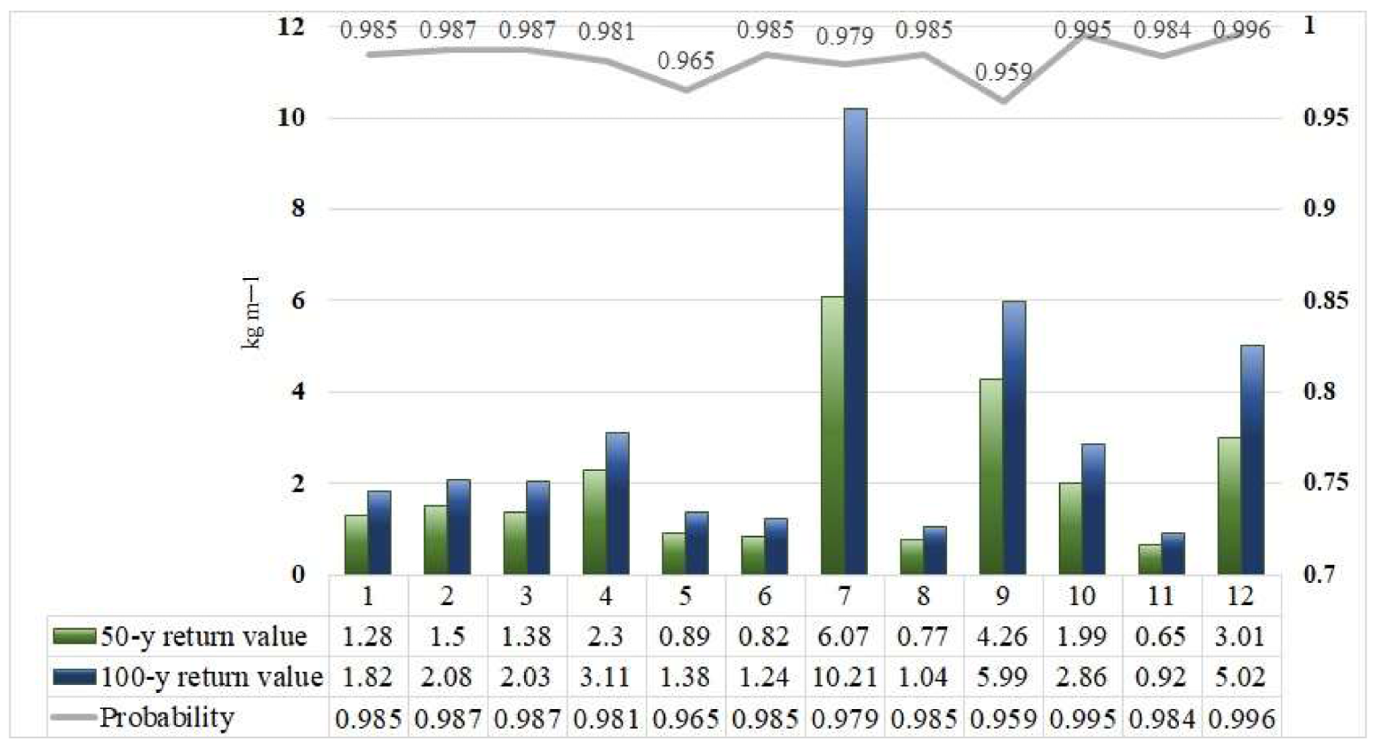
3.1. Return Period of Wet Snow Events

It is essential for professionals at the power supply companies to have the latest knowledge of the frequency and intensity of icing events, especially the return periods of external extra forces and extreme loads on the wires. In recent decades, several severe wet snow events were registered in the Carpathian Basin and the surrounding mountainous areas. In the last 15 years, the most significant wet snow cases with civil and media attention were in 2009, 2012, 2013, 2014, 2015, 2017, 2018 and 2021.

The Hungarian standards applicable to power system design were adapted to the climatic conditions of the 1970s and 1980s, but at that time there were not sufficiently long data series and sophisticated methods yet to calculate the extremes and their return periods. The POT method needs at least 20-year long observations [23]. The ISO 12494 [22] presented a classification of icing events based on its severity and the accumulated wet snow mass on the wires (

Table 4. International Ice Classes, and related mass (kg·m⁻¹) and diameter (cm) of accumulated wet snow on transmission overhead lines determined for two snow densities (300 kg m⁻³, 500 kg m⁻³) based on [22]. Calculated intervals are determined by Ducloux and Nygaard based on the 79% and 141% value of the diameter of snow sleeve (cm) as the lower and upper limits of the calculated intervals [60].

ISO International Ice Classes [22]	Snow Mass on the Wire (kg·m−1)	Diameter of Snow Sleeve (cm)		Calculated Intervals (kg·m−1) [60]
		(Diameter of Wire is 30 mm)
		Snow Density (kg·m−3)
		300	500
R1	0.5	5.5	4.7	0–0.70
R2	0.9	6.9	5.6	0.71–1.26
R3	1.6	8.8	7.1	1.27–2.25
R4	2.8	11.3	9.0	2.26–3.95
R5	5.0	14.9	11.7	3.96–7.05
R6	8.9	19.7	15.4	7.06–12.55
R7	16	26.2	20.4	12.56–22.55
R8	28	34.6	26.9	22.56–39.48
R9	50	46.2	35.8	39.49–70.50
R10	Extreme icing events			>70.51

). Ducloux and Nygaard [60] presented a mathematical approach to create intervals for ice classes in ISO 12494 in order to be able to objectively classify the calculated return values into the icing groups. According to this study, a good approximation of the minimum and maximum values of an Ice Class category (R1–R10) is the 79% and the 141% of the median value belonging to the given ice class (Table 4 Column “Snow mass on the wire (kg·m⁻¹)). For example, in the R2 category the minimum and maximum of the interval (Table 4 Column “Calculated intervals (kg·m⁻¹)”) is the 79% and 141% of the median value of R2 0.9 kg·m⁻¹. In the R1 category the minimum value practically has to be determined as zero. The intervals are not overlapping so they are suitable for classification.

Now we demonstrate the results of the extreme value analysis for two periods, 1965–1990 and 1991–2016.

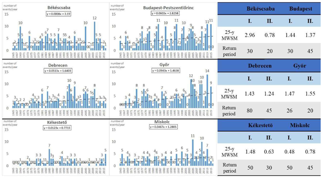
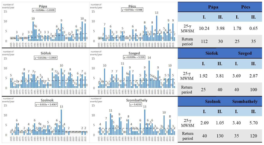
3.1.1. The Annual Frequency and 25-Year Maxima of Wet Snow Events

Firstly, the frequency of the annual number of wet snow events and their tendency were studied between 1965–2016. After the determination of wet snow events based on the conditions in Section 2.1, we defined the independent events using the following conditions: 1. a minimum of 24 precipitation-free hours passed between two snowfalls, or 2. a minimum of 6 h with air temperature above 2 °C and no snowfall. In this case, we assumed that the accreted snow sleeve melted from the wires due to high temperatures. However, owing to the low annual frequency of wet snow formation, this criterion was applied to a negligible extent. It is needed to emphasize again that the study is focusing on the complex atmospheric conditions that can lead to wet snow formation on wires, so the presented wet snow mass (kg·m⁻¹) is an estimated value calculated with Equations (1)–(9). We used visual observations of snowfall and measured meteorological parameters to determine the occurrence of wet snow events.

The Annual Number of Cases (ANC) of wet snow events by stations can be seen in Figure 7 and Figure 8 with the estimated values of 25-year Maximum Wet Snow Mass (kg·m⁻¹) and its return periods (years) between 1965–1990 (I. column in Figure 7 and Figure 8) and between 1991–2016 (II. column in Figure 7 and Figure 8).

According to the results of t-test (DF = 50, p = 0.05, t-critical = 2.0086) there was a significant increase in the Annual Number of Cases (ANC) in Budapest-Pestszentlőrinc, Debrecen, Győr, Kékestető, Miskolc, Pápa, Pécs, Siófok, Szeged. No significant trend can be indicated in Békéscsaba and Szombathely. A significant negative trend can be shown in Szolnok. The calculated Maximum Wet Snow Mass (MWSM) significantly decreased in Békéscsaba, Pápa and Szeged. There were no significant changes in Budapest-Pestszentlőrinc, Debrecen, Győr, Kékestető, Miskolc, Pécs, Siófok, Szolnok and Szombathely. The increased Annual Number of Cases and the insignificant changes in the Maximum Wet Snow Mass together indicate that the probability of heavier accumulations may have decreased (

Table 5. The Number of Cases (NC) between 1965–2016, the trend analysis of the Annual Number of Cases (ANC) based on Figure 7 and Figure 8 and of the calculated Maximum Wet Snow Mass (MWSM) in kg·m⁻¹ with t-test (p = 0.05) between 1965–2016. The critical t-value is 2.0086. Significant changes of the parameters are shaded with red (increase) or blue (decrease).

Station	NC (1965–2016)	Trend Analysis of ANC t-Value (p = 0.05)	Trend Analysis of MWSM t-Value (p = 0.05)
Békéscsaba	167	0.78	−2.24
Budapest-Pestszentlőrinc	230	77.6	−0.19
Debrecen	156	47.73	0.006
Győr	206	127.36	0.67
Kékestető	57	6.69	−0.03
Miskolc	131	42.98	−0.34
Pápa	129	57.08	−4.35
Pécs Pogány	148	80.25	−1.08
Siófok	195	13.13	0.73
Szeged	200	23.62	−2.1
Szolnok	106	−13.09	−0.73
Szombathely	178	0	−1.69

).

3.1.2. Return Period between 1965–1990 and 1991–2016

The length of the data series allowed us to split the whole period into a 24-year and a 25-year long period.

The Maximum Wet Snow Mass (kg·m⁻¹) of the first period (1965–1990) is presented in Figure 7 and Figure 8. The most exposed area was Pápa (25-year MWSM = 10.24 kg·m⁻¹). Its geographical location is favourable for wet snow formation, because the station is situated at the junction of a lowland (Kisalföld) and a hilly area (Bakony), while the most frequent wind direction during wet snow events is northwestern [13], so the station is on the windward side of the hilly area of Bakony. The return period of the 25-year maximum is 112 years (Figure 8), while the 50-year return value is 4.42 kg·m⁻¹ and the 100-year return value is 9.04 kg·m⁻¹ (Figure 9). It shows that the wet snow event which hit the station (25-year maximum) was an extremely rare event. Szombathely (25-year MWSM = 3.40 kg·m⁻¹, Figure 8) is in the western part of the country, which is one of the most exposed areas to wet snow formation in Hungary [61]. The 50-year return value (4.32 kg·m⁻¹) is almost equal to the value in Pápa (Figure 9). However, the 100-year return value does not reach the one in Pápa, but it is the second highest (6.54 kg·m⁻¹) among the studied stations. The stations on the Great Plains, i.e., Szeged, Békéscsaba and Szolnok (25-year MWSM = 3.69, 2.96 and 2.09 kg·m⁻¹, respectively), furthermore Pécs and Siófok (50-year return value = 3.06 and 2.67 kg·m⁻¹, respectively) are moderately endangered regions to wet snow accretion. The lowest values can be seen in Budapest-Pestszentlőrinc, Debrecen, Győr, Kékestető and Miskolc (25-year MWSM = 1.44, 1.43, 1.47, 1.48, 0.84 kg·m⁻¹, respectively in Figure 7 and Figure 8).

The spatial distribution of wet snow masses changed in the period of 1991–2016 (Figure 10). Although Szombathely and Pápa remained the most exposed areas, the 25-year Maximum Wet Snow Mass is lower than in the previous decades (5.70 kg·m⁻¹ and 3.98 kg·m⁻¹,respectively in Figure 7 and Figure 8). The severe exposure of Pápa is still reflected in the high values of 50-year and 100-year return values (6.07 kg·m⁻¹ and 10.21 kg·m⁻¹, respectively), which continue to be far ahead of the values of Szombathely (3.01 kg·m⁻¹ and 5.02 kg·m⁻¹, respectively) (Figure 10). Compared to the values in the previous period (1965–1990) it can be determined that a significant decrease in the 50-year return values can be seen in Békéscsaba, Kékestető, Pécs, Szeged, Szolnok, Szombathely. There is no significant change in Budapest-Pestszentlőrinc, Debrecen and Miskolc. A significant increase is confirmed in Győr, Pápa and Siófok. These stations are located in the northwestern part of the country.

3.2. Classification of Ice Classes

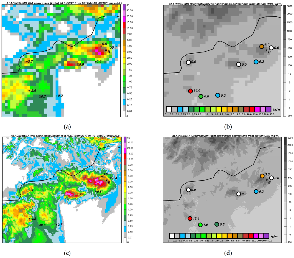
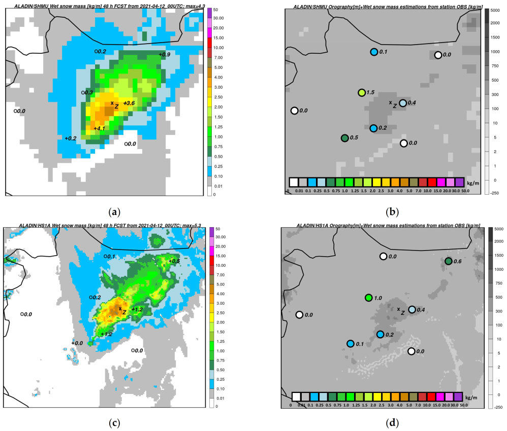
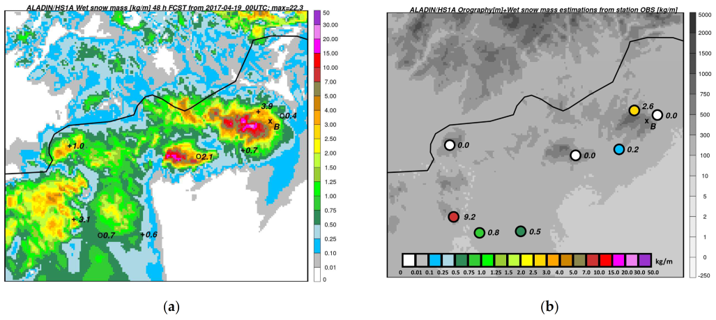
In order to enlighten the severity of the Ice Class categories and the exposure of the synoptical stations to the climatically possible wet snow masses, we used the classification of the international color codes of the warning system (green, yellow, orange, red), which is based on the expected danger or damages. The wet snow mass in the R1 and R2 ice classes does not mean potential danger to the transmission lines. The R3 ice class is low, while R4 and R5 categories are medium risks for the system. R6 and above categories meet the requirements of red warnings, so it means widespread and severe wet snow loads with breakdowns and blackouts affecting a significant number of the population [9].

In the first period a southwest-northeast gradient of severity can be seen in Figure 11a. However, wet snow is an exceptionally local phenomenon, the occurrence strongly depends on the momentary conditions of the atmosphere in a certain location, so spatial conclusions about climate characteristics can not be drawn based on the severity map. The only station without significant wet snow accumulation was Miskolc at this time. Low-risk stations were Budapest-Pestszentlőrinc, Debrecen, Győr and Kékestető. 7 out of the 12 stations belonged to the medium-risk categories (R4, R5). In the second period (Figure 11b) the rate of medium-risk stations decreased to 4, all located in the northwestern part of the country (Győr, Pápa, Siófok, Szombathely). The rate of no-risk stations increased from 1 to 4, these stations are Kékestető, Miskolc, Pécs and Szolnok. The low-risk categories are situated in the southeast part of the country (Békéscsaba, Debrecen, Szeged) and Budapest-Pestszentlőrinc (Figure 4b). Based only on the color codes representing the possible losses, there is no change of severity in Budapest, Debrecen, Miskolc, Pápa, Siófok, Szombathely. An increasing risk can be experienced only in Győr, while a reduction of risk can be seen in Békéscsaba, Kékestető, Pécs, Szeged, Szolnok (

Table 6. Comparison of Ice Classes [22].

Station	Label	Ice Class 1965–1990	Ice Class 1991–2016
Békéscsaba	1	R5	R3
Budapest	2	R3	R3
Debrecen	3	R3	R3
Győr	4	R3	R4
Kékestető	5	R3	R2
Miskolc	6	R2	R2
Pápa	7	R5	R5
Pécs	8	R4	R2
Siófok	9	R4	R5
Szeged	10	R5	R3
Szolnok	11	R4	R2
Szombathely	12	R5	R4

).

4. Case Studies

The calculation of the return period was possible from observations of 12 synoptic stations, which are mostly situated at lowland, with exception of the station Kékestető, which is near to the highest point of Hungary. However, wet snow events are often reported in the hill or mountain regions in the North and Northwest of Hungary. Two cases are presented here to illustrate the spatial distribution of wet snow mass in such situations and the possibility of analyzing them with aid of station observations and numerical models.

The first case occurred on 19–20 April 2017, when heavy precipitation (up to 80 mm in these two days, measured by precipitation gauges) and moderate-to-strong wind occurred at many places in Hungary [62]. In lowland, there was typically rain or snow with too high water content to accrete on wires (forming slush). Conditions for wet snow were favorable in mountains, where both station observations and numerical models indicated very high snow mass with maxima estimated about 14–34 kg·m⁻¹ (Figure 12a,b in ALADIN/SHMU and Figure 12c,d in ALADIN/HS1A). This would classify the event as R7-R8 according to the International Ice Class (an extreme ice event). There was also a direct observation and report about damages on electric wires due to wet snow in the village Bükkszentkereszt [63]. Wet snow events of this intensity are rare in Hungary. For comparison, a maximum wet snow mass between 1965–1990 was registered in Pápa (10.24 kg·m⁻¹) with a quite long return period of 112 years (refer to Figure 8).

The second event was less severe with respect to the estimated snow mass magnitudes (substantial damage was not claimed) and it occurred on 12–13 April 2021. Snow with a depth of 10–30 cm was reported from the Bakony mountains in the northwest of Hungary [64], and wet snow occurred in the city of Zirc. Numerical simulations indicated 4–5 kg·m⁻¹ snow accumulation (Figure 13a,b for ALADIN/SHMU and Figure 13c,d for ALADIN/HS1A), which would rate the event as class R5.

In both cases, there were neither synoptic, nor AWS measurements in the area of the highest snow masses predicted with ALADIN/SHMU or ALADIN/HS1A runs. These were situated in forest areas. In the case of 19–20 April 2017 snowfall, masses exceeding 10 kg·m⁻¹ were concentrated to relatively small zones (with dimensions of 10–20 km) at the slopes of Mátra and Bükk mountains. Meteorological stations could be rather found at the edges of these territories or at the top of the mountains.

In the ALADIN/HS1A numerical simulation of this case, local minima were placed to the highest points of Mátra or Börzsöny mountains, which agrees with the estimations of Kékestető and Nagy-Hideg-hegy stations. Here, the 2m temperature was mostly below the lower threshold for wet snow (−0.5 °C). This effect was absent in the 4.5 km resolution ALADIN/SHMU model, which orography is less accurate. Additionally, measurements of other stations (e.g., Budapest János-hegy, Miskolc Szentlélek, etc.) indicated that the temperature conditions for wet snow accretion were favorable only in certain intervals of heights—nearly between 200 and 800 m a.s.l. (Figure 14).

Unfortunately, there were no observations from the southern slopes of Mátra or Bükk mountains, where both models placed the highest snow mass, but were also quantitatively very different (two times higher mass in ALADIN/HS1A compared to ALADIN/SHMU model). The inaccuracy in the wet snow mass forecasts could be estimated to 1–3 kg·m⁻¹ (see the MAE of

Table 7. Evaluation of forecast errors of the ALADIN/SHMU and ALADIN/HS1A model runs for respective parameters—average 2 m temperature (°C) and 10 m wind (m·s⁻¹), total precipitation (mm), wet snow mass (kg·m⁻¹) in the case of the 19–20 April 2017 snowfall.

Parameter	2 m Temperature		10 m Wind		Total Precipitation		Wet Snow Mass
	SHMU	HS1A	SHMU	HS1A	SHMU	HS1A	SHMU	HS1A
BIAS	1.16	0.65	1.42	1.44	−29.41	−25.5	0.3	−0.36
MAE	1.21	0.73	2.8	2.17	29.86	26	3.13	1.85

). This is high in light of the fact that wet snow mass of 3 kg·m⁻¹ is already a threshold for 2nd level of warning (orange) in Hungary for this meteorological phenomenon [9]. The more exact forecasts of temperature, wind and precipitation resulted in smaller absolute error of snow mass in the higher resolution model run (ALADIN/HS1A).

In the 12–13 April 2021 situation the snow mass forecasts of both model runs were closer concerning magnitude and also the forecast errors of T2m, U10m, P were similar in magnitude in the ALADIN/SHMU and ALADIN/HS1A (

Table 8. The same as in Table 7, except for the 12–13 April 2021 snowfall.

Parameter	2 m Temperature		10 m Wind		Total Precipitation		Wet Snow Mass
	SHMU	HS1A	SHMU	HS1A	SHMU	HS1A	SHMU	HS1A
BIAS	0.71	0.77	1.32	1.37	−0.27	−5.1	0.84	0.1
MAE	0.75	0.77	2.27	2.41	9.1	10.1	1.22	0.37

). Comparison of the two snowfall events indicates that the accuracy of the model and the verification results can largely depend on the type of the situation, terrain (much flatter in the second studied case) and choice of the verifying stations (how much they are close to areas of high precipitation).

Experiments showed that for every input parameter (T2m, U10m, P) the accuracy of its determination had a high impact on the resulting snow mass estimates. For example, replacing observed 2 m temperature with model forecast could lead in ~2.5 kg·m⁻¹ increase in snow mass if using ALADIN/HS1A model data and even to ~8 kg·m⁻¹ in case of the ALADIN/SHMU with coarser resolution (

Table 9. Impact of respective parameters (2 m temperature, 10 m wind, precipitation) on the accuracy of wet snow mass (kg·m⁻¹) calculation in case the observed values were replaced by model forecasts (ALADIN/SHMU and ALADIN/HS1A) in the 19–20 April 2017 snowfall. Note that the results for “All” (all parameters replaced by model data) are slightly different from the wet snow mass forecast error in Table 7 because of the different integration time-step (1 h) compared to inline model calculations (36 s).

Observation Replaced by Model Data	Temperature		Wind		Precipitation		All
	SHMU	HS1A	SHMU	HS1A	SHMU	HS1A	SHMU	HS1A
BIAS	7.06	2.32	0.21	−0.04	−1.49	−1.43	0.39	−0.37
MAE	7.85	2.48	2.68	1.75	1.58	1.56	3.15	1.79

). For wind and precipitation the sensitivity was not as high but still a deviation of about 1.5–1.7 kg·m⁻¹ (or even 2.7 kg·m⁻¹) was possible when applying ALADIN/HS1A (ALADIN/SHMU) outputs. In the 12–13 April 2021 case the mean influence of replacing observed data by forecast ones was smaller but still up to 1–1.6 kg·m⁻¹ differences could be found in the case of temperature (

Table 10. As in Table 9 but for the 12–13 April 2021 snowfall.

Observation Replaced by Model Data	Temperature		Wind		Precipitation		All
	SHMU	HS1A	SHMU	HS1A	SHMU	HS1A	SHMU	HS1A
BIAS	1.42	1.07	0.06	0.07	−0.11	−0.15	0.84	0.1
MAE	1.62	1.14	0.08	0.09	0.23	0.19	1.22	0.37

).

For observation-based precipitation and snow mass estimates, the allowance of wind-induced undercatch effect can play an important role. It could be demonstrated in the 19–20 April 2017 case at several stations (

Table 11. Impact of the correction on wind on wet snow precipitation (P_w [mm]) estimates and of the limitation applied on wind (maximum wind speed = 7.5 m·s⁻¹) in Equation (8) after Goodison [31]. Resulting estimates of wet snow mass (M (kg·m⁻¹)) are listed for the respective approaches (no correction on wind, correction applied, correction with wind speed limit). Values were rounded to two decimals. All calculations are valid for the wet snow event of 19–20 April 2017. (NC = not corrected, C = corrected, N.U.L = no wind speed limit, U_max = 7.5 m s⁻¹).

Label	Name	Height a.s.l. [m]	Pw [mm] NC	Pw [mm] C, N.U.L	Pw [mm] C, Umax	M [kg m−1] NC	M [kg m−1] C, N.U.L	M [kg m−1] C, Umax
2	Budapest-Pestszentlőrinc	139	11.07	13.55	13.55	0.74	0.98	0.98
6	Miskolc	162	0	0	0	0	0	0
A9	Sülysáp	181	5.64	7.5	7.5	0.36	0.52	0.52
A2	Eger	225	3.27	3.72	3.72	0.18	0.21	0.21
A10	Budapest Zugliget	421	26	26	26	4.26	4.26	4.26
A1	Budapest János-hegy	516	17.44	41.22	38.57	3.09	13.38	11.8
A3	Miskolc Szentlélek	752	22.72	31.16	31.16	2.14	3.53	3.53
A4	Nagy-Hideg hegy	855	0.45	0.6	0.6	0.02	0.03	0.03
5	Kékestető	1012	0	0	0	0	0	0

). The correction increased the estimated snow mass, in case of the Budapest János-hegy station, by almost 10 kg·m⁻¹, due to high wind speed. However, it is uncertain whether the correction formula is still applicable for high wind speed at the gauge height. Experiments with limiting the wind to 7.5 m·s⁻¹ indicated that the snow mass calculation was sensitive to such changes if there was strong wind. In similar situations even a relatively small increase in precipitation could significantly amplify the snow mass due to strong flux. The extreme example of this effect was found at the Budapest János-hegy station. When not using the wind limit, the precipitation would be higher by ~2.7 mm but this would already result in snow mass higher by ~1.6 kg·m⁻¹ (which would mean more than 10 percent of the entire mass).

In the 12–13 April 2021 situation the impact of the undercatch correction was also relatively large -increasing two-times the masses at some stations (

Table 12. As in Table 11, but for the wet snow event of 12–13 April 2021.

Label	Name	Height a.s.l. [m]	Pw [mm] NC	Pw [mm] C, N.U.L	Pw [mm] C, Umax	M [kg m−1] NC	M [kg m−1] C, N.U.L	M [kg m−1] C, Umax
9	Siófok	108	0	0	0	0	0	0
4	Győr	117	0.73	0.82	0.82	0.04	0.04	0.04
7	Pápa	145	4.9	8.76	8.68	0.46	1.02	1.00
A7	Sümeg	195	0.95	1.52	1.52	0.06	0.10	0.10
12	Szombathely	201	0	0	0	0	0	0
A8	Tés	472	2.35	4.42	4.42	0.17	0.36	0.36
A6	Kab-hegy	595	0.88	2.39	2.05	0.08	0.24	0.20
A5	Gerecse tető	620	4.74	7.87	7.87	0.33	0.65	0.65

). On the other hand, the effect of the wind-limitation was below 0.1 kg·m⁻¹ and could come into question only at a few stations (e.g., at the top of the Kab-hegy mountain).

Additional experiments were done with setting the wet snow density to 500 kg·m⁻³ as the density of wet snow usually increases with higher wind speed [23]. As a consequence, output wet snow mass forecasts decreased considerably in the case of the 19–20 April 2017 snowfall (Figure 15a) when compared to reference calculations using 300 kg·m⁻³ density (shown in Figure 12c). With higher density value, the peak snow mass would be 9 kg·m⁻¹ from the AWS measurement estimations and 22 kg·m⁻¹ from the ALADIN/HS1A model simulation, which would correspond to the ice class of R6-R7. In the case of the 12–13 April 2021 snowfall the maximum predicted snow mass would decrease to 4 kg·m⁻¹ (class R5) (Figure 16). In both cases, the increase of wet snow density resulted in a drop of the snow mass estimations by nearly 30%.

5. Discussion

The results of the climatological examination show that the frequency of wet snow occurrences between the 1965–1990 and 1991–2016 periods has increased in 10 out of 12 stations. It is emphasized once more that the selection of wet snow occurrences is based on a special combination of weather parameters like visual observations of precipitation type (synoptic codes: 70 s) and 2 m temperature. The most significant changes in frequency can be seen in Pécs (112.5%), Győr (70%), Pápa (65%), Miskolc (55.7%) and Debrecen (42%). The 25-year Maximum Wet Snow Mass has decreased in Békéscsaba (73.6%), Pécs (63.5%), Kékestető (57.44%) and in Szolnok (49.7%). A moderate reduction in the wet snow mass maxima can be observed in Szeged, Budapest, Miskolc and Debrecen. The MWSM has increased in Northwest Hungary, especially in Pápa (220%) and Szombathely (67%). The highest Ice Class indicated by a 50-year return period calculation for the 12 stations was R5. Based on the results of spatial distribution and the return values it can be concluded that the exposure to severe wet snow masses has decreased in the south (Békéscsaba, Szeged, Szolnok, Pécs). There is no significant change in the Ice Classes in the central and northeast parts of the country, i.e., in Budapest, Debrecen, Miskolc. The most exposed areas with elevated risk are in the northwest part of Hungary, particularly in Pápa and Siófok.

However, it is probable that the most extreme wet snow events occur locally, in mountain areas of Hungary, where even Ice Classes of R6-R8 are possible. This concerns territories in the North and Northwest of Hungary (Bakony, Börzsöny, Mátra, Bükk) but possibly also some other parts of Hungary (e.g., western border with Austria or Mecsek mountains in the south of Hungary), which had not previously been mentioned. This is indicated by numerical simulations and two cases presented in this paper. There is no direct or indirect observational evidence of such high snow masses in mountains as were the peak values forecast by the models, because surface observations are rather sparse there.

Estimation of wet snow mass is very sensitive to parameterizations of wind-effects on snow accretion and precipitation. For the stations selected in the return period calculation, the wet snow and strong wind combination occurred rarely (1% of the wet snow cases). In case of high wind speed one should count with the fact that the uncertainty in specifying wet snow mass increases. First, the density of accreted snow can well exceed values of 300 or 400 kg·m⁻³ used in this study or in other return period calculations (e.g., [60]). When increasing this parameter, the accreted snow mass becomes substantially lower, as it was shown in the experiment with 500 kg·m⁻³ density for wet snow (Figure 15 and Figure 16). Unfortunately, there exist only very few observations of wet snow density in Hungary, which could help to specify the density-wind relationship in such situations.

Another potential source of inaccuracy is the parameterization of collection efficiency (beta). The parametrization of Admirat et al. [33], Admirat and Sakamoto [34] significantly underestimate the wet snow mass, while Nygaard et al. [29] and Sakamoto and Miura [28] overestimate the wet snow mass, especially in low wind conditions. The return period calculations using all the mentioned beta parametrizations and comparisons can be found in the work of Somfalvi-Tóth [13].

Ice or wet snow can be accreted on both rotational and sonic anemometers, which can increase the inaccuracy of wind measurements, above all in severe icing situations [65]. At the OMSZ stations, heating and protection of the anemometer shaft from icing started to be implemented from 1993 on automatic weather stations [66]. Heating of cups is also used at certain stations (e.g., Kékestető). Impact of wet snow on wind measurements could be expected above all in a case with strong wind, e.g., which appeared during the 19–20 April 2017 snowfall. However, anomalies in the course of the wind speed/wind direction, which would indicate this kind of problem were not found in data used for this case study.

The correction method of precipitation gauge data by strong wind also remains a problem, which cannot be satisfactorily solved without field experiments or direct precipitation and snow mass observations. Upon presented case studies it could be stated that the influence of the correction with the equation (8) was strong and the uncertainty (potential inaccuracy) in determining wet snow mass could be up to several kg m⁻¹ in extreme situations. From comparisons of NWP model forecasts and corrected precipitation observations one could hypothesize that the use of the above-mentioned formula perhaps even overestimated precipitation in conditions with strong wind. This is suggested by high underestimations of model precipitation during the 19–20 April 2017 snowfall when compared with corrected precipitation measurements (see the large negative mean BIAS in Table 7 for total precipitation). This negative BIAS was produced mainly at mountain stations (e.g., Budapest János-hegy, Kékestető), where the 10 m wind speed reached 10–14 m·s⁻¹. However, the NWP model forecast errors of precipitation are typically high in extreme situations, often due to spatial displacements between forecast and observed values, differences between the model and real topography, etc.

6. Conclusions

The extreme value analysis provided an estimation of climatological extremes of wet snow in Hungary, whom 50-year return period typically yielded 0.7–6.1 kg·m⁻¹. The highest snow mass appeared at the station Pápa, in northwestern Hungary at the foot of the Bakony mountains. Similar range of wet snow mass (0.3 and 8.3 kg·m⁻¹) was found in the return period calculation of the study for the area of France [60] despite its different climate zones (due to proximity of the Atlantic ocean and Mediterranean sea). Their extremes of 7–8 kg·m⁻¹ appeared in mountain areas of France or in the proximity of mountains. Severe wet snow cases in Hungary and numerical simulations also indicated that the highest snow mass might occur in mountain territory (at Bükk, Mátra or Bakony mountains). Deeper understanding of the differences or similarities between respective wet snow climates would require further research and also unification of the wet snow parameterization, which is different in the respective studies [60,67].

The comparisons of the two 25 year periods (1965–1990 and 1991–2016) showed that the wet snow climate at the examined station was evolving and decreasing tendencies (in southern and central Hungary) as well as areas with rising risk of wet snow (western part of Hungary) were found. This information was missing from former researches, which were less systematic, focused on case studies and did not cover all regions of Hungary.

Advantage of the extreme value analysis based on data from synoptic stations can be seen in easy applicability to sites with sufficiently long (at least 20 years) series of measurements of 2 m temperature, 10 m wind speed, precipitation amount and precipitation type. Thus, similar research could be extended also to other countries in the Pannonian Basin and applied to their observation network. The disadvantage of the method is that the number and the spatial coverage of stations suitable for the analysis is rather low, thus certain extremes of small areal extent could be missed. The case studies indicated that these extreme wet snow conditions (snow mass estimated with NWP models as high as 30–40 kg·m⁻¹) were present in the mountain regions of Hungary at heights between 200 and 800 m, while wet snow was only marginally appearing in lowlands at the same time. In contrast to most of the cases analysed during the return period calculations, these events occurred in an environment with strong wind, which resulted in higher uncertainty concerning the precipitation flux, snow density and other parameters in the wet snow mass calculation.

Such extremes could be analyzed using NWP models but due to small (typically below 20 km) areal extent of the most extreme snow mass values, horizontal resolution of about 1 km is preferable. This is above all important for steep mountain slopes, where model orography alters by several tens or hundreds of meters from the real one. This can be one of the causes of large forecast errors, which can be in order of several kg·m⁻¹. Other causes can be inaccuracies in the initial and boundary conditions or in the used physical parameterizations. As indicated by previous studies [18,68], there are more chances to localize wet snow events or determine their intensity with ensemble prediction systems (EPS). However, the EPS use (especially at high resolution) requires high computational power. Mesoscale LAM EPS systems providing outputs at 2.5 km resolution started to be only recently (February 2020) used in short-range forecasting in Hungary [69].

In the future, extending the extreme value analysis for later years and periods (following 2016) would be interesting because of the higher number of stations. However, due to the continuously decreasing number of man-powered observations, new methods must be introduced to determine the precipitation type. In Hungary, disdrometers have been implemented at several synoptic and AWS stations [70], which could be used for this purpose. Another possibility is the improvement of precipitation-type diagnostics from analyses of numerical models [71] and their combination with AWS measurements.

References

1. Wakahama, G.; Kuroiwa, D.; Goto, K. Snow Accretion on Electric Wires and its Prevention. J. Glaciol. 1977, 19, 479–487. [Google Scholar] [CrossRef] [Green Version]
2. Sakamoto, Y. Snow accretion on overhead wires. Philos. Trans. R. Soc. London. Ser. A Math. Phys. Eng. Sci. 2000, 358, 2941–2970. [Google Scholar] [CrossRef]
3. Makkonen, L.; Wichura, B. Simulating wet-snow loads on power line cables by a simple model. Cold Reg. Sci. Technol. 2010, 61, 73–81. [Google Scholar] [CrossRef]
4. Dalle, B.; Admirat, P. Wet snow accretion on overhead lines with French report of experience. Cold Reg. Sci. Technol. 2011, 65, 43–51. [Google Scholar] [CrossRef]
5. Yamamoto, K.; Matsumiya, H.; Sato, K.; Nemoto, M.; Togashi, K.; Matsushima, H.; Sugimoto, S. Evaluation for characteristics of wet snow accretion on transmission lines—Establishment of an experimental method using a vertical plate. Cold Reg. Sci. Technol. 2020, 174, 103014. [Google Scholar] [CrossRef]
6. Poots, G.; Skelton, P.L.I. Thermodynamic models of wet-snow accretion: Axial growth and liquid water content on a fixed conductor. Int. J. Heat Fluid Flow 1995, 16, 43–49. [Google Scholar] [CrossRef]
7. Tóth, K.; Kolláth, K. A tapadó hóteher mennyiségi előrejelzése. Légkör 2009, 54, 10–14. (In Hungarian) [Google Scholar]
8. Bonelli, P.; Lacavalla, M.; Marcacci, P.; Mariani, G.; Stella, G. Wet snow hazard for power lines: A forecast and alert system applied in Italy. Nat. Hazard Earth Sys. 2011, 11, 2419–2431. [Google Scholar] [CrossRef]
9. Somfalvi-Tóth, K.; Simon, A.; Kolláth, K.; Dezső, Z. Forecasting of wet- and blowing snow in Hungary. Időjárás 2015, 119, 277–306. [Google Scholar]
10. Laforte, J.L.; Allaire, M.A.; Laflamme, J. State-of-the-art on power line de-icing. Atmos. Res. 1998, 46, 143–158. [Google Scholar] [CrossRef]
11. Paul, S.; Chang, J. Design of novel electromagnetic energy harvester to power a deicing robot and monitoring sensors for transmission lines. Energy Convers. Manag. 2009, 197, 111868. [Google Scholar] [CrossRef]
12. Kollár, L.E.; Farzaneh, M. Modeling Sudden Ice Shedding from Conductor Bundles. IEEE Trans. Power Deliv. 2013, 28, 604–611. [Google Scholar] [CrossRef]
13. Somfalvi-Tóth, K. A Nagyfeszültségű Felsővezeték Hálózatot Érő Veszélyes Tapadó Hó Felhalmozódások Vizsgálata, Modellezése És Integrálása Az Előrejelzői Gyakorlatba. Ph.D. Thesis, ELTE, Budapest, Hungary, 2019. (In Hungarian). [Google Scholar]
14. Sakakibara, D.; Nakamura, Y.; Kawashima, K.; Miura, S. Experimental result for snow accretion characteristics of communications cable. In Proceedings of the International Wire and Cable Symposium, Lake Buena Vista, FL, USA, 21–23 May 2007. [Google Scholar]
15. Fikke, S.; Ronsten, G.; Heimo, A.; Kunz, S.; Ostrozlik, M.; Persson, P.E.; Sabata, J.; Wareing, B.; Wichura, B.; Chum, J.; et al. COST 727: Atmospheric Icing on Structures Measurements and Data Collection in Icing: State of the Art, Veröffentlichung MeteoSchweiz Nr. 75, Bundesamt Für Meteorologie und Klimatologie; Meteo Schweiz: Zurich, Switzerland, 2007; pp. 1–115. Available online: https://www.meteoswiss.admin.ch/dam/jcr:070f7439-3435-4966-8cbd-db30bbf59137/cost727atmosphericicingonstructures.pdf (accessed on 13 December 2022).
16. Lacavalla, M.; Marcacci, P.; Freddo, A. Wet-snow activity research in Italy. In Proceedings of the International Workshop on Atmospheric Icing and Structures, Uppsala, Sweden, 28 June–3 July 2015. [Google Scholar]
17. Csomor, M. A zúzmara megfigyelése. Légkör 1975, 3, 70–71. (In Hungarian) [Google Scholar]
18. Szűcs, M.; Sepsi, P.; Simon, A. Hungary’s use of ECMWF ensemble boundary conditions. ECMWF Newsl. 2016, 148, 24–30. [Google Scholar] [CrossRef]
19. Tóth, K.; Lakatos, M.; Kolláth, K.; Fülöp, R.; Simon, A. Climatology and forecasting of severe wet snow icing in Hungary. In Proceedings of the 13th International Workshop on Atmospheric Icing of Structures, IWAIS XIII, Andermatt, Switzerland, 8–11 September 2009. [Google Scholar]
20. Radnóti, G.; Ajjaji, R.; Bubnová, R.; Caian, M.; Cordoneanu, E. The spectral limited area model Arpègè-Aladin. PWPR Rep. Ser. 1995, 7, 111–117. [Google Scholar]
21. Horányi, A.; Ihász, I.; Radnóti, G. ARPEGE-ALADIN: A numerical weather prediction model for Central Europe with the participation of the Hungarian Meteorological Service. Időjárás 1996, 100, 277–300. [Google Scholar]
22. ISO 12494; Atmospheric Icing of Structures. International Standardization Organisation (ISO): Geneva, Switzerland, 2001.
23. Farzaneh, M. Atmospheric Icing of Power Networks, 1st ed.; Springer: Dordrecht, The Netherlands, 2008; pp. 1–373. [Google Scholar]
24. Tozer, B.; Sandwell, D.T.; Smith, W.H.F.; Olson, C.; Beale, J.R.; Wessel, P. Global bathymetry and topography at 15 arc sec: SRTM15+. Earth Space Sci. 2019, 6, 1847–1864. [Google Scholar] [CrossRef]
25. Nikolov, D.; Makkonen, L. Testing Six Wet Snow Models by 30 Years of Observations in Bulgaria. In Proceedings of the International Workshop on Atmospheric Icing and Structures, Uppsala, Sweden, 28 June–3 July 2015. [Google Scholar]
26. Admirat, P. Wet Snow Accretion on Overhead lines. In Atmospheric Icing of Power Networks, 1st ed.; Farzaneh, M., Ed.; Springer: Dordrecht, The Netherlands, 2008; Volume 4, pp. 119–169. [Google Scholar] [CrossRef]
27. Finstad, K.; Fikke, J.; Ervik, M. A comprehensive deterministic model for transmission line icing applied to laboratory and field observations. In Proceedings of the International Workshop on Atmospheric Icing and Structures, Paris, France, 4–7 September 1988. [Google Scholar]
28. Sakamoto, Y.; Miura, A. Comparative study of wet snow models for estimating snow load on power lines based on general meteorological parameters. In Proceedings of the International Workshop on Atmospheric Icing and Structures, Budapest, Hungary, 20–23 September 1993. [Google Scholar]
29. Nygaard, B.E.K.; Ágústsson, H.; Somfalvi-Tóth, K. Modeling Wet Snow Accretion on Power Lines: Improvements to Previous Methods Using 50 Years of Observations. J. Appl. Meteor. Climatol. 2013, 52, 2189–2203. [Google Scholar] [CrossRef]
30. Rasmussen, R.; Baker, B.; Kochendorfer, J.; Myers, T.; Landolt, S.; Fisher, A.; Black, J.; Theriault, J.; Kucera, P.; Gochis, D.; et al. How well are we measuring snow? The NOAA/FAA/NCAR winter precipitation test bed. Bull. Am. Meteorol. Soc. 2012, 93, 811–829. [Google Scholar] [CrossRef] [Green Version]
31. Goodison, B.E.; Louie, P.Y.T.; Yang, D. WMO Solid Precipitation Measurement Intercomparison—Final Report. In Instruments and Observing Reports, 1st ed.; Goodison, B.E., Ed.; World Meteorological Organization: Geneva, Italy, 1998; Available online: https://library.wmo.int/index.php?lvl=notice_display&id=6441#.Y2Yzy3bMLIU (accessed on 30 December 2022).
32. Deneau, V.; Guillot, P. Wet-snow accretion on power lines: Cartographic examination of risks throughout France. Houille Blanche. 1984, 6, 465–474. [Google Scholar] [CrossRef] [Green Version]
33. Admirat, P.; Sakamoto, Y.; DeGoncourt, B. Calibration of a snow accumulation model based on actual cases in Japan and France. In Proceedings of the International Workshop on Atmospheric Icing and Structures, Paris, France, 4–7 September 1988. [Google Scholar]
34. Admirat, P.; Sakamoto, Y. Calibration of a wet-snow model on real cases in Japan and France. In Proceedings of the International Workshop on Atmospheric Icing and Structures, Paris, France, 4–7 September 1988. [Google Scholar]
35. Le Du, M.; Laurent, C. T-Return Period Values of Meteorological Design Parameters. In Proceedings of the International Workshop on Atmospheric Icing and Structures, Montreal, QC, Canada, 12–16 June 2005. [Google Scholar]
36. Lakatos, M.; Bihari, Z. Hóteher a távvezetékeken. A 2009. január 27–28-án kialakult időjárási helyzet elemzése Vas és Zala megye területén. Légkör 2009, 54, 6–9. (In Hungarian) [Google Scholar]
37. Coles, S. An Introduction to Statistical Modeling of Extreme Values, 1st ed.; Springer: London, UK, 2001; Volume 4, pp. 74–91. [Google Scholar] [CrossRef]
38. Lakatos, M.; Matyasovszky, I. Analysis of the extremity of precipitation intensity using the POT method. Időjárás 2004, 108, 155–208. [Google Scholar]
39. Ribatet, M. POT: Modelling peaks over a threshold. R News 2007, 7, 34–36. [Google Scholar]
40. Termonia, P.; Fischer, C.; Bazile, E.; Bouyssel, F.; Brožková, R.; Bénard, P.; Bochenek, B.; Degrauwe, D.; Derková, M.; El Khatib, R.; et al. The ALADIN System and its Canonical Model Configurations AROME CY41T1 and ALARO CY40T1. Geosci. Model Dev. 2018, 11, 257–281. [Google Scholar] [CrossRef] [Green Version]
41. El Khatib, R. Fullpos Users Guide for Arpege/Aladin Cycle 25T1; Météo France—CNRM/GMAP: Toulouse, France, 2002; p. 68. Available online: https://confluence.ecmwf.int/download/attachments/19661682/fullpos_usersguide_cy25y1.pdf (accessed on 12 December 2022).
42. Derková, M.; Vivoda, J.; Belluš, M.; Španiel, O.; Dian, M.; Neštiak, M.; Zehnal, R. Recent Improvements in the ALADIN/SHMU Operational System. Meteorol. J. 2017, 20, 45–52. Available online: https://www.shmu.sk/File/ExtraFiles/MET_CASOPIS/2017-2__MC.pdf (accessed on 5 November 2022).
43. Simon, A.; Belluš, M.; Čatlošová, K.; Derková, M.; Dian, M.; Imrišek, M.; Kaňák, J.; Méri, L.; Neštiak, M.; Vivoda, J. Numerical simulations of June 7, 2020 convective precipitation over Slovakia using deterministic, probabilistic, and convection-permitting approaches. Idojaras 2021, 125, 571–607. [Google Scholar] [CrossRef]
44. Taillefer, F.; CANARI Technical Documentation. Based on ARPEGE Cycle CY25T1 (AL25T1 for ALADIN); CNRM/GMAP Meteo France. 2002. Available online: http://www.cnrm.meteo.fr/gmapdoc/spip.php?article3 (accessed on 5 November 2022).
45. Courtier, P.; Geleyn, J.-F. A global numerical weather prediction model with variable resolution: Application to the shallow model equations. Quart. J. Roy. Meteor. Soc. 1988, 114, 1321–1346. [Google Scholar] [CrossRef]
46. Courtier, P.; Freydier, C.; Geleyn, J.-F.; Rabier, F.; Rochas, M. The ARPEGE project at Météo-France. In Proceedings of the 1991 ECMWF Seminar on Numerical Methods in Atmospheric Models, ECMWF, Reading, UK, 9–13 September 1991; pp. 193–231. [Google Scholar]
47. Simmons, A.J.; Burridge, D. An energy and angularmomentum conserving vertical finite-difference scheme and hybrid vertical coordinates. Mon. Weather Rev. 1981, 109, 758–766. [Google Scholar] [CrossRef]
48. Hortal, M. The development and testing of a new two-time-level semi-Lagrangian scheme (SETTLS) in the ECMWF forecast model. Quart. J. Roy. Meteorol. Soc. 2002, 128, 1671–1687. [Google Scholar] [CrossRef]
49. Bénard, P.; Vivoda, J.; Mašek, J.; Smolíková, P.; Yessad, K.; Smith, C.; Brožková, R.; Geleyn, J.F. Dynamical kernel of the Aladin–NH spectral limited-area model: Revised formulation and sensitivity experiments. Quart. J. Roy. Meteor. Soc. 2010, 136, 155–169. [Google Scholar] [CrossRef]
50. Ďurán, I.B.; Geleyn, J.; Váňa, F. A Compact Model for the Stability Dependency of TKE Production–Destruction–Conversion Terms Valid for the Whole Range of Richardson Numbers. J. Atmos. Sci. 2014, 71, 3004–3026. [Google Scholar] [CrossRef]
51. Ďurán, I.B.; Geleyn, J.; Váňa, F.; Schmidli, J.; Brožková, R. A Turbulence Scheme with Two Prognostic Turbulence Energies. J. Atmos. Sci. 2018, 75, 3381–3402. [Google Scholar] [CrossRef]
52. Gerard, L.; Piriou, J.-M.; Brožková, R.; Geleyn, J.-F.; Banciu, D. Cloud and precipitation parameterization in a meso-gamma scale operational weather prediction model. Mon. Weather Rev. 2009, 137, 3960–3977. [Google Scholar] [CrossRef]
53. Lopez, P. Implementation and validation of a new prognostic large-scale cloud and precipitation scheme for climate and data assimilation purposes. Quart. J. Roy. Meteor. Soc. 2002, 128, 229–257. [Google Scholar] [CrossRef]
54. Noilhan, J.; Planton, S. A simple parameterization of land surface processes for meteorological models. Mon. Weather Rev. 1989, 117, 536–549. [Google Scholar] [CrossRef]
55. Masson, V.; Champeaux, J.-L.; Chauvin, F.; Meriguet, C.; Lacaze, R. A Global Database of Land Surface Parameters at 1-km Resolution in Meteorological and Climate Models. J. Clim. 2003, 16, 1261–1282. [Google Scholar] [CrossRef]
56. Faroux, S.; Masson, V.; Roujean, J.-L. ECOCLIMAP-II: A climatologic global data base of ecosystems and land surface parameters at 1 km based on the analysis of time series of VEGETATION data. In Proceedings of the 2007 IEEE International Geoscience and Remote Sensing Symposium, Barcelona, Spain, 23–28 July 2007; pp. 1008–1011. [Google Scholar] [CrossRef]
57. Brožková, R.; Bučánek, A.; Mašek, J.; Smolíková, P.; Trojáková, A. Nová provozní konfigurace modelu Aladin ve vysokém rozlišení. Meteorol. Zprávy 2019, 72, 129–139. Available online: http://www.cmes.cz/sites/default/files/chmu_mz_5-19_129-139.pdf (accessed on 5 November 2022).
58. Brožková, R.; Bučánek, A.; Mašek, J.; Němec, D.; Smolíková, P.; Šábik, F.; Trojáková, A. Numerical Weather Prediction Activities at CHMI. In Proceedings of the ACCORD 1st AWS, Video Conference, 12–16 April 2021; Available online: http://www.umr-cnrm.fr/accord/IMG/pdf/poster_asw_2021_cz.pdf (accessed on 5 November 2022).
59. Huai, B.; Broeke, M.R.; Reijmer, C.H.; Cappellen, J. Quantifying Rainfall in Greenland: A Combined Observational and Modeling Approach. J. Appl. Meteor. Climatol. 2021, 60, 1171–1188. [Google Scholar] [CrossRef]
60. Ducloux, H.; Nygaard, B.E. 50-year return-period wet-snow load estimation based on weather station data for overhead line design in France. Nat. Hazards Earth Syst. Sci. 2014, 14, 3031–3041. [Google Scholar] [CrossRef] [Green Version]
61. Gulyás, K. A Tapadó Hó Statisztikus Klimatológiai Vizsgálata És Előrejelzési Lehetőségei. Master’s Thesis, ELTE, Budapest, Hungary, 2012. [Google Scholar]
62. OMSZ. Magyarország Időjárása (Daily Weather Report of 20 April 2017, In Hungarian); Országos Meteorológiai Szolgálat. Available online: https://owww.met.hu/idojaras/aktualis_idojaras/napijelentes_2005-2019/main.php?ts=1492646400&ful=napijelentes_szoveg (accessed on 5 November 2022).
63. Erdődiné Molnár, Z.; (OMSZ, Bükkszentkereszt, Hungary); Simon, A.; (OMSZ, Budapest, Hungary). Personal communication, 2017.
64. OMSZ. Időjárás Napijelentés (Daily Weather Report of 14 April 2021, In Hungarian); Országos Meteorológiai Szolgálat. Available online: https://met.hu/downloads.php?id=20&file=20210414&type=1 (accessed on 5 November 2022).
65. Makkonen, L.; Lehtonen, P.; Helle, L. Anemometry in Icing Conditions. J. Atmos. Oceanic Technol. 2001, 18, 1457–1469. [Google Scholar] [CrossRef]
66. Tóth, R.; (OMSZ, Budapest, Hungary); Simon, A.; (OMSZ, Budapest, Hungary). Personal communication, 2022.
67. Lacavalla, M.; Sperati, S.; Bonanno, R.; Marcacci, P. A Revision of Wet Snow Load Map for the Italian Power Lines with a New High Resolution Reanalysis Dataset. In Proceedings of the International Workshop on Atmopheric Icing of Structures, IWAIS, Reykjavík, Iceland, 23–28 June 2019; Available online: https://iwais2019.is/images/Papers/012_IWAIS2019_complete_paper_Lacavalla.pdf (accessed on 13 December 2022).
68. Simon, A.; Somfalvi-Tóth, K.; Szűcs, M. Probabilistic forecasting of freezing rain and wet snow in Hungary. In Proceedings of the EMS Annual Meeting: European Conference for Applied Meteorology and Climatology, Budapest, Hungary, 2–7 September 2018. [Google Scholar]
69. Lancz, D.; Jávorné Radnóczi, K.; Szanyi, K.; Szepszo, G.; Szintai, B.; Tóth, B.; Tóth, G.; Tóth, H.; Várkonyi, A. NWP activities at the Hungarian Meteorological Service. In Proceedings of the 44th EWGLAM–29th SRNWP Workshop, Brussels, Belgium, 26–29 September 2022. [Google Scholar]
70. Ablonczy, D. How Do We Measure the Rain? How Strong is the Sun Now? How Does the Anemometer Work? Meteorological Instruments Simply in Practice. Légkör 2018, 63, 163–177. [Google Scholar]
71. Gascón, E.; Hewson, T.; Haiden, T. Improving Predictions of Precipitation Type at the Surface: Description and Verification of Two New Products from the ECMWF Ensemble. Wea. Forecast. 2018, 33, 89–108. [Google Scholar] [CrossRef]
Figure 1. Photographs of wet snow accreted on power lines and poles (a) at Bükkszentkereszt on 20 April 2017 (courtesy of István Erdődi), the diameter of accreted snow sleeve was estimated between 7 and 8 cm, (b) near Budapest János-hegy on 19 April 2017 (photo by André Simon).
Atmosphere 14 00081 g001
Figure 2. Flow chart of the applied methods and results. The abbreviations T2m, U10m and P mean 2 m temperature, 10 m wind and precipitation amount, respectively.
Atmosphere 14 00081 g002
Figure 3. Map with positions of OMSZ synoptic weather stations used for wet snow climatology and return period calculation (circles, numbers 1–12, see Table 1). Positions of AWS stations selected for the wet snow case studies of 19–20 April 2017 and 12–13 April 2021 are highlighted by “plus” symbols and denoted A1–A8 (see Table 2). Positions of observed wet snow accretion at Zirc (Z) and Bükkszentkereszt (B) are marked with X. Some mountains mentioned in the text (Bükk, Mátra, Bakony, etc.) are also displayed. The background is orography (in m a.s.l.) from a subset of the SRTM15+ database [24]. The map depicts area between 15° E, 45° N (southwestern corner) and 24° E, 49° N (northeastern corner).
Atmosphere 14 00081 g003
Figure 4. Example of the selection of threshold (a) MRL Plot and (b) Dispersion Index Plot in Pápa between 1991–2016. The grey lines in the MRL Plot are the minimum and maximum values of the 95% confidence interval.
Atmosphere 14 00081 g004
Figure 5. Example of the goodness of fit test of (a) Probability Plot and (b) Q-Q Plot with the 95% confidence interval (dashed lines) in Pápa between 1991–2016 to prove the goodness of the chosen threshold. The distribution of wet snow mass data [kg·m−1] above the threshold follow the Pareto distribution.
Atmosphere 14 00081 g005
Figure 6. (a) Domain and orography (in m a.s.l.) of the ALADIN/SHMU model. The HS1A rectangle shows the position and size of the domain for the high resolution runs. The map depicts area between 2.32° E, 33.78° N (southwestern corner) and 39.05° E, 55.87° N (northeastern corner); (b) as in (a) but for the ALADIN/HS1A high resolution model version. The rectangles show the position and size of regions shown in Figures in the Section 4, concerning wet snow situations of 19–20 April 2017 (right rectangle) and 12–13 April 2021 (left rectangle). The map depicts area between 14.69° E, 45.17° N (southwestern corner) and 24.18° E, 50.23° N (northeastern corner).
Atmosphere 14 00081 g006
Figure 7. Annual Number of Cases (ANC) of wet snow events between 1965–2016 with a linear trend line (dotted line) and its equation (left) and the 25-year Maximum Wet Snow Mass (MWSM) (kg·m−1) and its Return period in the 1965–1990 period (Column I.) and in the 1991–2016 period (Column II.) (right) in Békéscsaba, Budapest-Pestszentlőrinc, Debrecen, Győr, Kékestető, Miskolc.
Atmosphere 14 00081 g007
Figure 8. Annual Number of Cases (ANC) of wet snow events between 1965–2016 with a linear trend line (dotted line) and its equation (left) and the 25-year Maximum Wet Snow Mass (MWSM) (kg·m−1) and its Return period in the 1965–1990 period (Column I.) and in the 1991–2016 period (Column II.) (right) in Pápa, Pécs, Siófok, Szeged, Szolnok, Szombathely.
Atmosphere 14 00081 g008
Figure 9. 50-year and 100-year return value of wet snow mass (kg·m−1) and the probability of the 50-year return value calculated from the estimated wet snow mass (kg·m−1) between 1965–1990. See the explanation of station labels 1–12 in Table 1.
Atmosphere 14 00081 g009
Figure 10. 50-year and 100-year return value of wet snow mass (kg·m−1) and the probability of the 50-year return value calculated from the estimated wet snow mass (kg·m−1) between 1991–2016. See the explanation of station labels 1–12 in Table 1.
Atmosphere 14 00081 g010
Figure 11. Categories of International Ice Classes [22] on Hungarian synoptic stations between (a) 1965–1990 and (b) 1991–2016. The colors represent the severity of climatically possible wet snow masses based on the international color scale of the warning system. Station labels can be seen in Table 1. The map depicts area between 15° E, 45° N (southwestern corner) and 24° E, 49° N (northeastern corner).
Atmosphere 14 00081 g011
Figure 12. (a) Forecast of cumulated wet snow mass (shaded, kg·m−1) from the ALADIN/SHMU run based on 19 April 2017 00 UTC and valid for 21 April 2017 00 UTC in the region of northern Hungary (domain shown in Figure 6b). Circles, plus “and X” symbols depict the positions of stations and sites as explained in Figure 3. The numbers are model forecasts of the mass valid for the closest grid-point of height corresponding to station height.; (b) ALADIN/SHMU model orography (shaded, m). Numbers and colored circles show the mass (kg·m−1) estimated from both station observations and ALADIN/SHMU data and cumulated for the same period as in a).; (c) as in (a) but for the ALADIN/HS1A model run.; (d) as in (b) but for estimations using ALADIN/HS1A inputs.
Atmosphere 14 00081 g012
Figure 13. (a) Forecast of cumulated wet snow mass (shaded, kg·m−1) from the ALADIN/SHMU run based on 12 April 2021 00 UTC and valid for 14 April 2021 00 UTC in the region of northwestern Hungary (domain shown in Figure 6b). The meaning of numbers and symbols is the same as in Figure 3 and Figure 12; (b) ALADIN/SHMU model orography (shaded, m). Numbers and colored circles show the mass (kg·m−1) estimated from both station observations and NWP data and cumulated for the same period as in (a).; (c) as in (a) but for the ALADIN/HS1A model run.; (d) as in (b) but for estimations using ALADIN/HS1A inputs.
Atmosphere 14 00081 g013
Figure 14. Variation of 2 m average temperature (solid line, °C) and estimated wet snow mass (dashed line, 101 kg·m−1) with station height (m) during the case of 19–20 April 2017. The profiles were constructed from measurements of synoptic and AWS stations. Averaging of temperature was applied for the period of precipitation at each station. The shaded rectangle emphasizes the range of temperature, where wet snow was considered (−0.5, 2 °C).
Atmosphere 14 00081 g014
Figure 15. (a) Forecast of cumulated wet snow mass (shaded, kg·m−1) from the ALADIN/HS1A run based on 19 April 2017 00 UTC and valid for 21 April 2017 00 UTC in the region of northern Hungary from an experiment defining density of wet snow as 500 kg·m−3. Meaning of numbers and characters as in Figure 12 and Figure 13; (b) ALADIN/HS1A model orography (m). Numbers and colored circles show the mass (kg·m−1) estimated from both station observations and NWP data and cumulated for the same period and with the same setup of wet snow density as in (a). Compare with Figure 12c,d for the wet snow density of 300 kg·m−3.
Atmosphere 14 00081 g015
Figure 16. (a) as in Figure 15a but for the run based on 12 April 2021 00 UTC and valid for 14 April 2021 00 UTC and for northwestern Hungary.; (b) ALADIN/HS1A model orography (shaded, m). Numbers represent the station observation and NWP-based estimations of wet snow mass (kg·m−1) cumulated for the same period and with the same setup of wet snow density (500 kg·m−3) as in (a). Compare with the reference ALADIN/HS1A results presented in Figure 13c,d.
Atmosphere 14 00081 g016