Article

Seasonal Lifting Condensation Level Trends: Implications of Warming and Reforestation in Appalachia’s Deciduous Forest

1
National Weather Service, National Oceanic and Atmospheric Administration, 112 Airpark Drive South, Negaunee, MI 49866, USA
2
Division of Forestry and Natural Resources, Davis College of Agriculture, Natural Resources and Design, West Virginia University, Morgantown, WV 26506, USA
*
Author to whom correspondence should be addressed.
Atmosphere 2023, 14(1), 98; https://doi.org/10.3390/atmos14010098
Submission received: 1 December 2022 / Revised: 28 December 2022 / Accepted: 29 December 2022 / Published: 2 January 2023
(This article belongs to the Section Biosphere/Hydrosphere/Land–Atmosphere Interactions)

Abstract

:
Lifting condensation level (LCL) has long been used to estimate cloud base heights. However, spatial and temporal patterns of cloud bases embedded within atmospheric currents flowing over mountainous terrain still need to be more adequately described. To advance understanding, hourly observations of barometric pressure and ambient and dew point temperatures from 1948 to 2017 were acquired for seven airports located at 40.21° N (average) and crossing the Allegheny Mountains of the northeastern United States. Daily LCL trends were quantified, and large positive (2.3 m yr−1) and negative (−1.3 m yr−1) LCL trends were found to be greatest near seasonal transition dates (17 April and 9 November 2022). Cool season LCLs (795 m) increased significantly (p < 0.007) at five sites resulting in an average LCL increase of 81 m and implying a deeper and drier sub-cloud layer. Average warm season LCLs (773 m) decreased by 23 m, suggesting a deeper convective cloud layer and less sub-cloud evaporation that may facilitate higher hydrometeor growth and precipitation rates. Collective results indicate divergent seasonally averaged LCLs characterized by more rapid seasonal transitions, warmer and less cloudy cool seasons, and cloudier and more humid warm seasons that may be partly attributable to aggressive reforestation and contribute to more significant rainfall events and higher flood risks.

1. Introduction

Moist atmospheric currents flowing over mountainous terrain often result in orographic cloud and precipitation regimes across a spectrum of spatial and temporal scales [1,2]. Distributions of cloud cover, cloud base height (CBH), hydrometeor formation [3], growth [4,5], and sub-cloud evaporation [6] are influenced by cloud development near and across complex topography [7]. In addition to producing precipitation, cloud cover reduces incoming solar radiation (i.e., insolation; [8]), especially at low elevations where greater water vapor concentrations can increase cloud albedo [1,9]. Insolation (radiation budgets) is the primary energy source of evapotranspiration (ET; [10]). Therefore, changes in cloud cover, CBH, or both, are fundamental to the hydrologic partitioning of precipitation to ET and streamflow regimes in mountainous terrain where increasing flood frequency is of particular concern [11,12].
Lifting condensation level (LCL) is the height at which an air parcel reaches saturation if lifted adiabatically [13] and is a robust estimate of CBH [14]. LCL estimations include assumptions of constant mixing ratios and potential temperatures throughout the depth of a well-mixed boundary layer [15]. However, mixing ratios are commonly elevated in the lowest 1 km of the troposphere due to ET [16,17], horizontal moisture advection [18,19], and mesoscale orographic circulations [20]. Therefore, LCL calculations using surface observations provide a theoretical lower bound of CBHs, even when clouds are not present. LCLs are also more accurate than visually estimated CBH observations [15,21]. Fortunately, routine measurements of each variable in the exact expression for LCL (ambient temperature, relative humidity, and barometric pressure; [13]) began in the late 1940s at many United States airports [22]. This is important because changing CBHs [23] and ET rates [24] may contribute to observed increases in precipitation event frequency [25] and magnitude across the northeastern United States [26].
The Appalachian Mountain system (AMS) covers a significant geographic area of the northeastern United States where extensive reforestation occurred during the 20th century [27,28,29]. The AMS is characterized by decreasing temperature and increasing precipitation with elevation and a rain shadow to the east, but the region is becoming warmer with increasing precipitation [29,30,31]. A north–south gradient with increasing CBH north of 37.5° N was shown in a previous investigation of sites approximately parallel to the AMS [32], suggesting CBH trends along the AMS are associated with latitudinal insolation gradients. However, the mid-latitude atmospheric flow is often westerly, along the lines of constant latitude, and perpendicular to the AMS [1,8]. Therefore, quantifying CBH gradients and trends at a constant latitude is needed to advance the understanding of cloud climatology within mid-latitude mountainous regions, including the AMS. Additionally, intra-annual analyses may improve understanding seasonal phenology associated with warming temperatures and changing Appalachian cloud cover [33,34,35,36,37]. This work is important given that clouds are an important component of Earth’s climate system, and the current study will advance the statistical understanding of CBHs within the AMS. Additionally, rapid 19th and 20th-century reforestation suggest historic changes to the AMS climate system that could represent many geographical locations currently experiencing rapid land use globally.
The objective of the current work was to quantify LCL statistics at an hourly resolution between 1948 and 2017 for seven airports oriented approximately perpendicular to the Appalachian Mountains at 40.21° N ± 0.75° latitude. Sub-objectives included (a) quantifying daily LCL trends at each airport, (b) determining the magnitude, direction, and significance of seasonal LCL trends at each airport, and (c) modeling average daily changes between LCL and insolation.

2. Materials and Methods

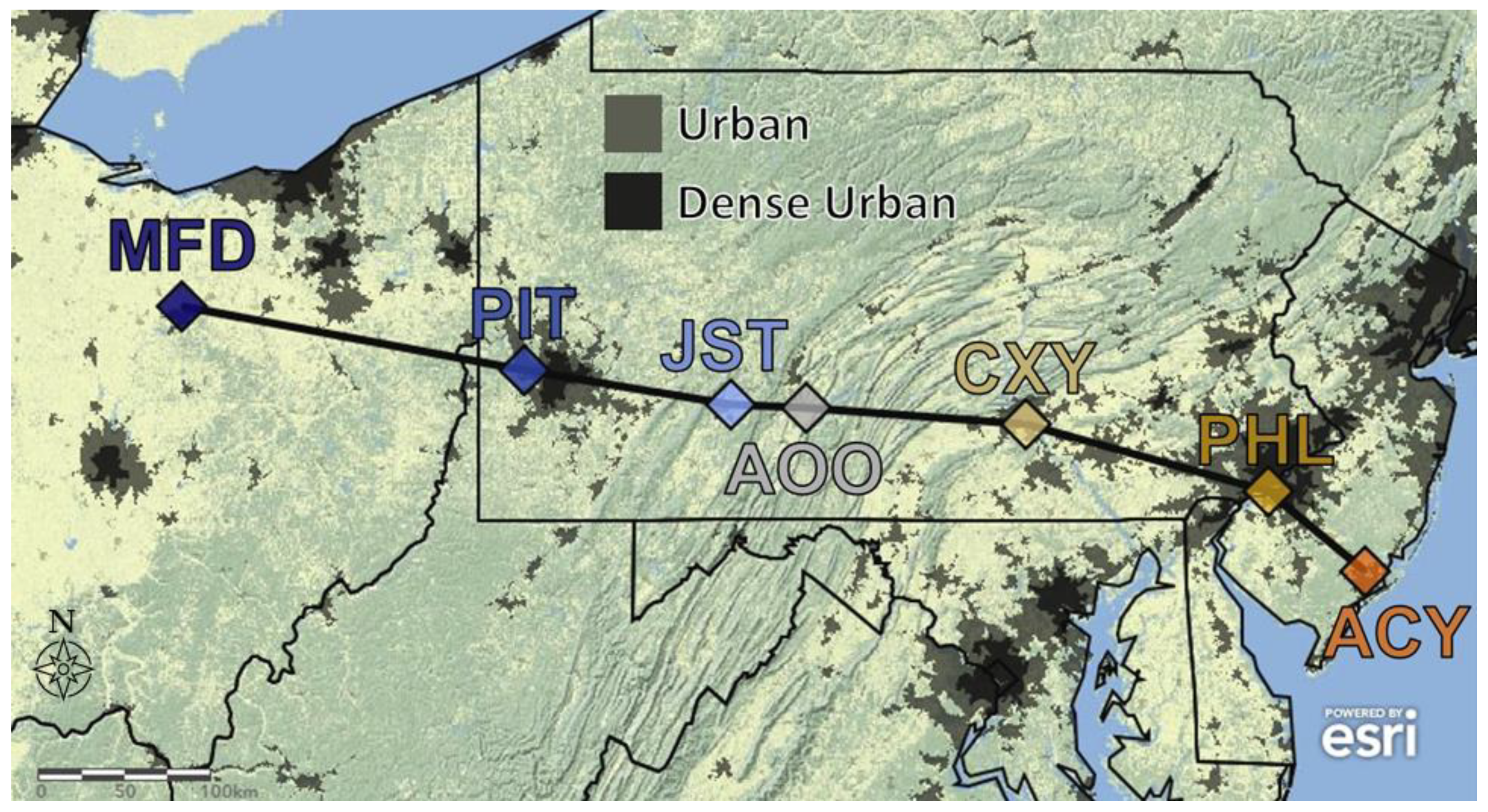
2.1. Site Description and Data Acquisition

Airports in Ohio (n = 1), Pennsylvania (n = 5), and New Jersey (n = 1), USA, were selected for the current work (Table 1). From here forward, the series of seven airports are referred to as the cross Appalachia transect (CAT; Figure 1). The seven CAT airports included the Mansfield Regional Airport (MFD), Pittsburgh International Airport (PIT), Johnstown-Cambria County Airport (JST), Altoona-Blair County Airport (AOO), Capital City Airport (CXY), Philadelphia International Airport (PHL), and Atlantic City International Airport (ACY; Figure 1; Table 1). Each airport was within 0.75° latitude of the CAT average (40.21° N), and from west to east, each airport’s latitude consistently decreased (Table 1). PIT and CXY were separated by just 0.27° latitude (39 km), minimizing latitudinal climatic gradients (i.e., insolation) where the CAT intersects the Allegheny Mountain Range within the broader AMS. The topographic profile of the CAT extended from the western edge of the Allegheny Plateau through each of the seven selected airports (Table 1) and terminated near the east coast at Atlantic City, New Jersey, USA (Figure 2a).
All available meteorological terminal aviation routine (METAR) weather reports for CAT sites were acquired from Iowa State University’s Iowa Environmental Mesonet (IEM) archive (https://mesonet.agron.iastate.edu/ (accessed on 1 July 2018); Table 1). During the late 20th century, METARs transitioned from quality-controlled observations made by certified observers (FCM-H1 2005) to automated surface observation systems subjected to quality control algorithms at three temporal or spatial scales [21]. In total, more than 3.4 million hourly observations of each variable were processed over 44- to 69-year periods of record that were used to quantify spatial LCL differences and temporal LCL trends (Table 1).

2.2. Data Processing

Ambient (Ta) and dew point (Td) temperature observations were used to quantify the relative humidity (RH) with respect to water (Ta > 0 °C) and ice (Ta ≤ 0 °C) using the Tetens’ formula [38,39]. Altimeter (Pa) observations were converted to station pressure (Pstn) using (1) where hm represents station elevation (Table 1).
P stn = P a [ ( 288 0.0065 × h m ) 288 ] 5.2561
Hourly values of Ta, RH, and Pstn were input into the exact expression for the lifting condensation level (LCL) detailed in [13] using R source code provided at https://romps.berkeley.edu/papers/pubdata/2016/lcl/lcl.R (accessed on 1 April 2019). The precise expression of LCL is accurate to within the uncertainty of vapor pressure measurements resulting in an LCL uncertainty of approximately ±5 m [13]. Hourly observations were averaged daily and seasonally to analyze the annual oscillation, the gradient across the Appalachian Mountains, and temporal trends in LCL height. Seasonal averages of LCL data were quantified for the dormant (November through April) and growing (May through October) seasons. The Mann–Kendall (MK) trend test was used to determine significant seasonal LCL trends at α = 0.05, and Sen’s slope estimator was used to quantify the linear trend at the 95% confidence interval using R software [40]. MK’s trend test is a non-parametric test that is less sensitive to outliers and skewed distributions than parametric approaches making MK appropriate for this work, e.g., [41]. Descriptive statistics of hourly LCL observations and linear trends of seasonally averaged LCL observations were quantified for each airport’s respective period of record using Origin Pro© software. Daily average insolation was calculated at 40.21° N using climlab version 0.7.0, a Python package for process-oriented climate modeling [42]. The geocontext application from the Center for Geographic Analysis was used to acquire topographic profile and distance data presented in Figure 2a [43].

3. Results and Discussion

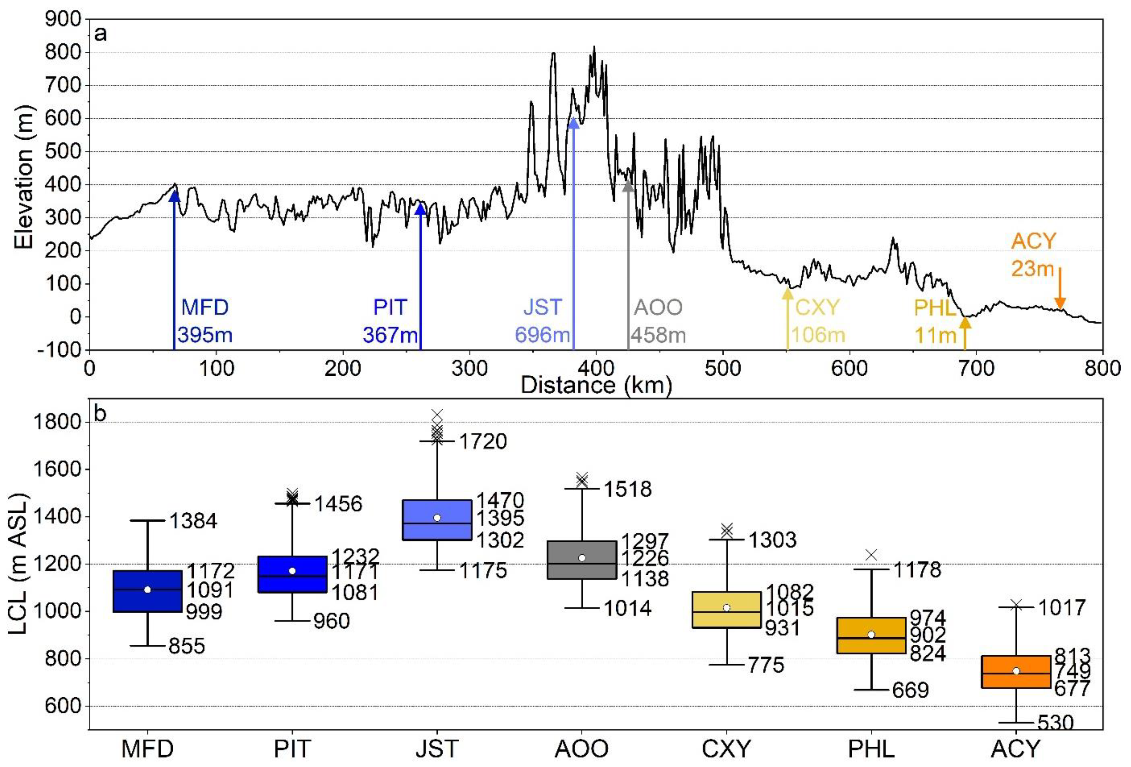
3.1. Appalachian LCL Climatology

Low-altitude clouds form when the depth of a well-mixed boundary layer increases beyond the LCL [44], which is rarely greater than a few kilometers [45]. The current work confirms this since maximum LCLs were between 4134 m (AOO) and 4556 m (ACY) after decades of routine observations (Table 2). Boundary layer depth is highly variable in time and space [44,45]. Still, CAT average LCLs in the current work were between 696 m (MFD) and 908 m (CXY), suggesting either a relatively shallow boundary layer, frequent low-altitude clouds, or both. Median LCL values were nearly identical at MFD (572 m), JST (570 m), and ACY (570 m), but values at airports in between were substantially higher (≥85 m). This is consistent with a mountain atmosphere that slopes gradually relative to the underlying terrain (Figure 2; [1,46]). For example, the range of mean LCLs (212 m; Table 2) was substantially smaller than the differences in airport elevation (685 m; Table 1).
Hourly lifting condensation level (LCL) observations were positively skewed (Table 2) at all seven airports suggesting nocturnal LCLs were farther below the mean than daytime LCLs were above the mean. Median LCL values averaged 119 m lower than mean LCL values along the CAT, and kurtosis was positive (i.e., leptokurtic) at six of the seven airports. Leptokurtic distributions indicate higher peaks (e.g., frequent low clouds) and heavier tails (e.g., spring maxima; Figure 3) consistent with more LCL variability than a normal distribution implies [47]. PHL’s LCL distribution was not leptokurtic and was the least skewed (Table 2), which may be a result of widespread urbanization (Figure 1; [48]) increasing surface temperatures and modulating local diurnal temperature oscillations [49]. Alternatively, LCLs at the highest elevation station (JST) was characterized by the largest skewness (1.10) and kurtosis (1.25; Table 2) consistent with frequent cloud immersion [34,50] and larger insolation values [9,51], respectively.

3.2. Cross Appalachian LCL Gradient

Longitudinal gradients in the range of average daily LCLs (Table 3) indicate intra-annual LCL variability increased with distance from the Atlantic Ocean (i.e., continentality). Except for PIT, inter-quartile ranges of daily mean LCL decreased from the west (MFD; 173 m) to the east (ACY; 136 m), consistent with an increasingly maritime climate [1]. Alternatively, the skewness of average intra-annual variability was greatest at JST, consistent with the most frequent cloud immersion [51] and decreased in both directions (Table 3). Kurtosis had a similar CAT gradient as skewness but became negative away from the AMS. Kurtosis was particularly negative (i.e., platykurtic) at MFD (−0.66), indicating less intra-annual LCL variability than normal distribution implies [47], which could be related to geographic proximity to Lake Erie (Figure 1). Outliers of average daily LCLs exceeding 1.5 standard deviations above the mean existed at all airports except MFD (Figure 2b) and occurred between 23 March and 27 April (not shown). These dates corresponded with the annual minimum in relative humidity that occurs near and before the transition from primarily evaporation to evapotranspiration (i.e., spring green up; Figure 3; [52]). Feedbacks between the seasonality of surface fluxes (i.e., transpiration) and cloud formation are likely to amplify as Appalachia shifts toward a wetter and more humid climate with a longer growing season [31,53,54]. Changing cloud characteristics may also influence precipitation intensity, especially in mountainous regions such as Appalachia, where rugged terrain simultaneously focuses cloud development and flooding vulnerability [55,56,57]. Combined, longitudinal LCL gradients along the CAT indicate that LCL variability was influenced by elevation, distance from the Atlantic Ocean, and seasonality of boundary layer water vapor fluxes.

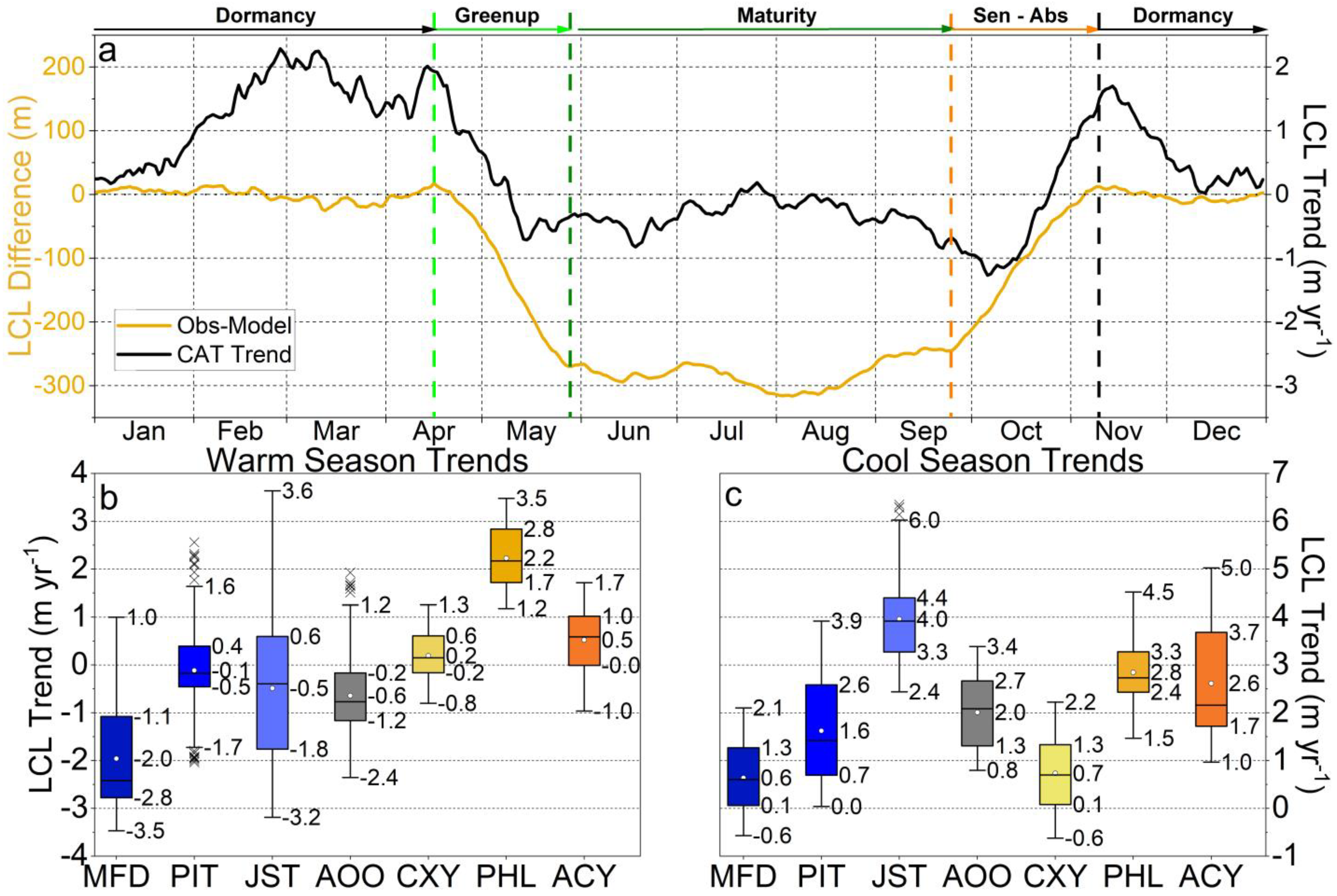
3.3. LCL Seasonality and Trends

Elevated moisture concentrations influence LCL estimations in the lowest 1 km of the boundary layer [15], which is often attributed to ET [16]. Among other variables, ET is a function of insolation and atmospheric saturation [58], and relative humidity (RH) is a standard method for quantifying partially saturated conditions [39]. Figure 3 shows CAT averages of RH, LCL, and insolation at 40.21° N averaged daily with three-week moving averages to smooth daily noise. The maximum smoothed daily average RH (73.9%) occurred on 24 September, and the minimum (61.2%) was on 15 April, whereas the highest average LCL (1020 m) was on 20 April, and the lowest (656 m) was 24 September. A secondary LCL maximum (758 m) occurred on 5 November when daily average insolation values were 197 W m−2, smaller than the springtime maximum. The dates of LCL maxima coincide with the beginning and end of the growing season for temperate deciduous forests of the northeastern United States [52]. In this work, the start (i.e., green up; 17 April) and end (i.e., dormancy; 9 November) of the growing season corresponded to the period of peak correlation between insolation and smoothed CAT average LCLs (R2 = 0.992; not shown). Vegetative maturity (29 May to 23 September) corresponded to dates of inflection points in Figure 4a. Therefore, METAR observations could help monitor local to regional phenology near airports globally.
Average LCLs decreased 197 m during the green-up stage (17 April to 27 May; Figure 3), indicating transpiration substantially reduces LCLs along the CAT. Lowering LCLs and increasing insolation during the green-up phase suggest more frequent opportunities for surface-based convective cloud and precipitation development [59]. Importantly, lower LCLs increase convective available potential energy and the potential for heavy convective rainfall rates that are increasing in magnitude faster than the Clausius-Clapeyron relation indicates (~6.5% °C−1; i.e., super-CC scaling; [60]). Smoothed average daily LCLs varied little (812 m ≤ LCL ≤ 838 m; average = 823 m) between 27 May and 3 July when leaves are mature and insolation is maximized (Figure 3). However, LCL values decreased 182 m between 3 July and 24 September, suggesting proportional decreases in LCL and insolation. Atmospheric currents on the western periphery of the Bermuda High also become moister as the Atlantic Ocean and Gulf of Mexico water temperatures reach their seasonal peaks [61]. Rapidly declining insolation during September suggests an optimal combination of low LCLs and large insolation values for heavy convective rainfall between the summer solstice and autumnal equinox [31]. July was characterized by the peak lightning strike frequency in Pennsylvania, USA, and thunderstorms dominate the envelope curve of flood peaks across the central Appalachian region [62]. Therefore, it is reasonable to assume that transpiration lowers summertime LCLs and may contribute to more frequent and more extensive convective precipitation rates.
Insolation and smoothed CAT average LCLs were highly correlated (R2 = 0.992; not shown) during the dormant season but were relatively weakly correlated throughout the entire year (R2 = 0.288). These seasonal differences are assumed to be caused by differences between evaporation-dominated vegetative dormancy and combined evaporation and transpiration (ET) during the growing season [58,63]. Using a linear model of LCL calibrated during the dormant season with insolation as the independent variable enables the estimation of transpiration induced LCL reductions (Figure 4a). Differences between observed and modeled LCL values indicate ET reduced LCLs by more than 100 m between 7 May and 17 October. The maximum difference was −316 m on 6 August, less than two weeks after the maximum CAT average precipitation rate [31]. 6 August is also 47 days after the summer solstice suggesting poleward advection of subtropical moisture plumes compensated for decreasing insolation [64,65]. However, substantial year-to-year variability (data not shown) indicates long periods of record are needed better to understand ET within the soil-plant-atmosphere continuum [66].
Convective cloud and precipitation development are favored when LCLs are low, and insolation and ET are large [59,67]. Differences between modeled and observed LCLs decreased 71 m between 6 August and 24 September, with a more rapid 251 m decrease between 24 September and 6 November (Figure 4a). Increasing humid and cloudy late summer air masses [61,65] and decreasing insolation combined to limit potential ET during August and September, whereas leaf senescence and abscission (i.e., coloration and removal) during October ended transpiration [52,68]. These findings are important considering changes in regional scale vegetative species composition, land cover (including afforestation), reforestation of marginal lands for energy crops, and plant water availability may feedback into seasonal characteristics, including cloud cover, LCLs, rainfall, and growing season length [31,36,69].
Linear trends of smoothed daily LCLs indicate prominent positive trends (1.1 m yr−1) during vegetative dormancy relative to the negative trends (−0.4 m yr−1) during active vegetative growth (Figure 4a). Seasonally dependent LCL trends are consistent with global trends in cloud base height [23]. The maximum smoothed daily LCL trend (2.3 m yr−1) occurred on 28 February, and the minimum LCL trend (−1.3 m yr−1) occurred on 6 October. Sharply decreasing trends during green-up and sharply increasing trends during senescence and abscission imply more rapid seasonal transitions that may contribute to a lengthening growing season [69]. Decreasing LCL trends often occurred during summer months when minor LCL differences can differentiate convective precipitation development from a capping inversion, preventing cloud cover [20]. Lowering LCLs may be relevant to super-CC scaling [60] by increasing hydrometeor growth and reducing sub-cloud evaporation [4,5,6]. Reforestation and/or afforestation of marginally productive (i.e., former mining or agricultural) lands across Appalachia’s rugged landscape may exacerbate LCL trends and subsequent vulnerabilities to heavy rainfall [31]. CAT average LCL trends ultimately raise cool season LCLs, lower warm season LCLs, and more rapid seasonal transitions with potential implications for super-CC scaling of convective rainfall.
Daily LCL trends at each airport for warm (Figure 4b) and cool seasons (Figure 4c) and seasonally averaged LCL trends (Table 4) indicate longitudinal gradients along the CAT. During the warm season, LCL trends were largest (2.2 m yr−1) at PHL and smallest (−2.5 m yr−1) at MFD, and both trends were significant (p ≤ 0.011; Table 4). Each site’s average LCL increased during the cool season (10 November to 17 April), and significant increases (p ≤ 0.011) were found at five airports (Table 4). Increasing LCLs suggest a warmer, drier, and deeper boundary layer with fewer highly reflective low-altitude clouds. Decreasing LCLs suggest a cooler, more humid, and shallower boundary layer that facilitates cloud development. The average cool season LCL (781 m) increased 81 m, and the most significant increasing trend occurred at JST, where cool season LCLs increased an estimated 160 m since 1973. Average warm season LCL (788 m) decreased 23 m, but decreasing trends were only significant at MFD (−2.5 m yr−1), where warm season LCL decreased 158 m since 1948 (Table 4). Similar seasonal averages combined with diverging seasonal trends indicate that average cool-season LCLs increased above warm-season LCL averages during this study’s period of record. Significantly increasing (p < 0.001) cool season LCLs at PHL and ACY (Table 4) could be attributed to urbanization [70], especially when considering PHL’s metropolitan population increased by 2.6 million residents between 1950 and 2013 [48]. Increasing warm season LCLs further suggests less frequent urban cloud cover that could increase the severity of extreme heat waves in many cities globally, e.g., [71].

3.4. Implications of Warming and Reforestation in Appalachia

Since the early 20th century, the Appalachian eastern deciduous forest (EDF) aggressively reforested as agricultural land uses shifted west [29]. It was estimated that Appalachia’s areal forest cover increased by 38% between 1920 and 1949 [29] when agricultural management practices across the Great Plains contributed to the 1930s Dust Bowl and the 1950’s Texas Drought [72,73]. Center pivot irrigation was patented in 1952 and proliferated the Great Plains during the 1960s and 1970s [74], during which time Appalachia shifted toward a more temperate, humid, and wetter climate [29]. This investigation builds on previous work showing that from 1948 to 2017, temperatures warmed, precipitation increased, and reforestation rates slowed as the EDF matured and timber volume increased [28]. These systematic shifts are consistent with increasing soil moisture that is negatively correlated with LCL height [75,76,77]. Climatic changes, among other factors, shifted forest species succession toward diffuse porous species (e.g., maple) adapted to damp and shady environments [29,36]. Cloud characteristics influence above-canopy light quality such that tree species commonly referred to as ‘shade-tolerant’ may be adapted to cloudy climates and canopy shading (understory). Extensive Appalachian land use change may therefore synergize with warming temperatures and increasing precipitation to enhance integrated soil-plant-atmosphere feedbacks.
Changing climate system characteristics, including cloud coverage, cloud base height, temperature, and moisture content, have important implications for two distinct but interactive areas of ongoing research: heavy precipitation (i.e., flooding) and ecosystem biodiversity. The influence of mountain barriers on short-duration extreme convective precipitation rates is particularly concerning because steep slopes focus convective cloud and precipitation development [20] and increase flooding vulnerabilities [11]. In the current work, warm season LCLs decreased at five CAT airports indicating warmer cloud bases with greater water vapor concentrations that may be consistent with positive feedback between latent heat release and precipitation rates (i.e., super-CC scaling; [60]). Lowering warm season LCLs implies changing thermodynamics (e.g., CAPE and CIN; [15]), faster hydrometeor growth rates [5], and reduced sub-cloud evaporation [6]. However, the relative importance of changes in large-scale precipitation regimes versus mesoscale boundary layer processes such as mechanical convection, differential heating of complex terrain, and convective cloud initiation remains to be determined. Warmer nighttime minimum temperatures suggest warmer dew points and heavier nocturnal dewfall that could amplify diurnal latent heat fluxes of a well-watered forest canopy [29]. Understanding changes in latent heat fluxes (e.g., ET) and ecosystem biodiversity should therefore be investigated further in the context of changing precipitation regimes.
Across North America’s EDF, the growing season is lengthening [78], and the species composition is shifting with important implications for water resources [79]. Drought-intolerant and shade-tolerant species are becoming more abundant [36,80] within an increasingly humid, wet, and temperate Appalachian climate system [29]. The EDF’s biodiversity may be adapting to changing cloud characteristics (i.e., light quality and quantity; [51]), increased plant available water resources [25], and other interactive forest disturbances, including pests and pathogens [36]. More specifically, cool season LCLs increased significantly (p < 0.007) at five CAT airports indicating a warmer, less humid, and deeper boundary layer that may influence the prevalence of pests and pathogens. Collectively, seasonal LCL trends along the CAT suggest biodiversity of montane ecosystems within the AMS are particularly vulnerable to changing CBHs [34]. Additionally, LCL trends were maximized near seasonal transition dates indicating more rapid seasonal transitions that could be important for regional agriculture, ecosystem productivity, recreation, and tourism. Multiple directions of future work exist including an assessment of the relative importance of boundary layer processes for cloud characteristics that have important implications for heavy precipitation and ecological biodiversity across the EDF.

4. Conclusions

Hourly METAR reports were collected between 1948 and 2017 at seven airports crossing the Appalachian Mountains. Hourly LCLs were then quantified to improve understanding of regional LCL climatology, spatial LCL gradients, and sub-seasonal LCL trends. Positively skewed and leptokurtic distributions were found at each airport, indicating less diurnal LCL variability than a normal distribution implying frequent low clouds, fog, and dew along the CAT. Elevation-dependent CBH, temperature and moisture content differences sloped more gradually than underlying terrain with important implications for local water budgets, ecosystem biodiversity, and carbon assimilation rates. Smoothed LCLs and insolation were strongly correlated during the cool season (R2 = 0.992) but were comparatively weakly correlated throughout the year (R2 = 0.288). Positive and negative LCL trends were greatest near seasonal transition dates (17 April and 9 November), indicating increasingly rapid seasonal transitions. Significantly increasing (p < 0.007) cool season LCLs were identified at five of the seven airports (CAT average 81 m increase), indicating a deepening boundary layer where turbulent mixing removes heat and moisture from the landscape. The relationship between LCL, insolation, and ET is particularly noteworthy during the warm season since a longer growing season may similarly lengthen the time of year when super-CC scaling of convective precipitation rates is possible. For example, CAT average warm season LCL trends decreased 23 m, indicating changing thermodynamics (e.g., CAPE and CIN), faster hydrometeor growth rates (latent heat release), and reduced sub-cloud evaporation. However, further work is needed to examine the relative importance of specific mechanisms and thresholds associated with changing LCLs and super-CC scaling of short-duration precipitation extremes. The current work advances the understanding of sub-seasonal trends in LCL that have critical and interrelated hydrological and ecological implications.

Author Contributions

Conceptualization, E.K. and J.A.H.; methodology, E.K. and J.A.H.; validation, E.K.; formal analysis, E.K.; investigation, E.K.; resources, J.A.H.; data curation, E.K.; writing—original draft preparation, E.K.; writing—review and editing, J.A.H.; visualization, E.K.; supervision, J.A.H.; project administration, J.A.H.; funding acquisition, J.A.H. All authors have read and agreed to the published version of the manuscript.

Funding

This work was supported by the USDA National Institute of Food and Agriculture, Hatch project accession number 1011536 and McIntire Stennis accession number 7003934, and the West Virginia Agricultural and Forestry Experiment Station. Additional funding was provided by the USDA Natural Resources Conservation Service, Soil and Water conservation, Environmental Quality Incentives Program No: 68-3D47-18-005, and a portion of this research was supported by Agriculture and Food Research Initiative Competitive Grant no. 2020-68012-31881 from the USDA National Institute of Food and Agriculture. Results presented may not reflect the views of the sponsors and no official endorsement should be inferred. The funders had no role in the study design, data collection, analysis, decision to publish, or preparation of the manuscript.

Institutional Review Board Statement

Not applicable.

Informed Consent Statement

Not applicable.

Data Availability Statement

All hourly METAR data is available via Iowa State University’s Iowa Environmental Mesonet at: https://mesonet.agron.iastate.edu/request/download.phtml (accessed on 1 July 2018). R script used for downloading METAR data via the database linked above: https://github.com/realmiketalbot/R-scripts/blob/master/iem_scraper_example.r (accessed on 1 July 2018). R script for calculating the exact expression of LCL used in this work: https://romps.berkeley.edu/papers/pubdata/2016/lcl/lcl.R (accessed on 1 April 2019).

Acknowledgments

The authors appreciate the support of many scientists of the Interdisciplinary Hydrology Laboratory (https://www.researchgate.net/lab/The-Interdisciplinary-Hydrology-Laboratory-Jason-A-Hubbart; accessed on 20 October 2022). The authors also appreciate the feedback of anonymous reviewers whose constructive comments improved the article.

Conflicts of Interest

The authors declare no conflict of interest.

References

  1. Barry, R.G. Mountains and their climatological study. In Mountain Weather and Climate, 3rd ed.; Cambridge University Press: New York, NY, USA, 2008; pp. 1–23. ISBN 978-0-521-68158-2. [Google Scholar]
  2. Martucci, G.; Milroy, C.; O’Dowd, C.D. Detection of cloud-base height using Jenoptik CHM15K and Vaisala CL31 ceilometers. J. Atmos. Ocean. Technol. 2010, 27, 305–318. [Google Scholar] [CrossRef]
  3. Rogers, A.D.; Yau, B.E. Formation of Cloud Droplets. In A Short Course in Cloud Physics, 3rd ed.; Butterworth-Heinemann: Burlington, MA, USA, 1989; pp. 81–98. ISBN 0-7506-3215-1. [Google Scholar]
  4. Medina, S.; Houze, R.A., Jr. Air motions and precipitation growth in Alpine storms. Quart. J. Roy. Meteor. Soc. 2003, 129, 345–371. [Google Scholar] [CrossRef] [Green Version]
  5. Fuchs, B.R.; Rutledge, S.A.; Bruning, E.C.; Pierce, J.R.; Kodros, J.K.; Lang, T.J.; MacGorman, D.R.; Krehbiel, P.R.; Rison, W. Environmental controls on storm intensity and charge structure in multiple regions of the continental United States. J. Geophys. Res. Atmos. 2015, 120, 6575–6596. [Google Scholar] [CrossRef]
  6. Houze, R.A., Jr. Clouds in tropical cyclones. Mon. Wea. Rev. 2010, 138, 293–344. [Google Scholar] [CrossRef]
  7. Georgis, J.F.; Roux, F.; Chong, M.; Pradier, S. Triple-Doppler radar analysis of the heavy rain event observed in the Lago Maggiore region during MAP IOP 2b. Quart. J. Roy. Meteor. Soc. 2003, 129, 495–522. [Google Scholar] [CrossRef]
  8. Petty, G.W. Properties of Radiation. In A First Course in Atmospheric Radiation, 2nd ed.; Sundog Publishing: Madison, WI, USA, 2006; p. 52. ISBN 978-0-9729033-1-8. [Google Scholar]
  9. Müller, H. On the radiation budget in the Alps. Int. J. Climatol. 1985, 5, 445–462. [Google Scholar] [CrossRef]
  10. Anderson, M.; Diak, G.; Gao, F.; Knipper, K.; Hain, C.; Eichelmann, E.; Hemes, K.S.; Baldocchi, D.; Kustas, W.; Yang, Y. Impact of Insolation Data Source on Remote Sensing Retrievals of Evapotranspiration over the California Delta. Remote Sens. 2019, 11, 216. [Google Scholar] [CrossRef] [Green Version]
  11. Rasmussen, K.L.; Houze, R., Jr. A. A flash-flooding storm at the steep edge of high terrain: Disaster in the Himalayas. Bull. Am. Meteorol. Soc. 2012, 93, 1713–1724. [Google Scholar] [CrossRef] [Green Version]
  12. Dottori, F.; Szewczyk, W.; Ciscar, J.C.; Zhao, F.; Alfieri, L.; Hirabayahi, Y.; Bianchi, A.; Mongelli, I.; Frieler, K.; Betts, R.A.; et al. Increased human and economic losses from river flooding with anthropogenic warming. Nat. Clim. Chang. 2018, 8, 781–786. [Google Scholar] [CrossRef]
  13. Romps, D.M. Exact Expression for the Lifting Condensation Level. J. Atmos. Sci. 2017, 74, 3891–3900. [Google Scholar] [CrossRef]
  14. Stackpole, J.D. Numerical analysis of atmospheric soundings. J. Appl. Meteor. 1967, 6, 464–467. [Google Scholar] [CrossRef]
  15. Craven, J.P.; Jewell, R.E.; Brooks, H.E. Comparison between observed convective cloud-base heights and lifting condensation level for two different lifted parcels. Wea. Forecast. 2002, 17, 885–890. [Google Scholar] [CrossRef]
  16. Melfi, S.H.; Whiteman, D. Observation of lower-atmospheric moisture structure and its evolution using a Raman lidar. Bull. Am. Meteorol. Soc. 1985, 66, 1288–1292. [Google Scholar] [CrossRef]
  17. Pinty, J.P.; Mascart, P.; Richard, E.; Rosset, R. An investigation of mesoscale flows induced by vegetation inhomogeneities using an evapotranspiration model calibrated against HAPEX-MOBILHY data. J. Appl. Meteor. 1989, 28, 976–992. [Google Scholar] [CrossRef]
  18. Helfand, H.M.; Schubert, S.D. Climatology of the simulated Great Plains low-level jet and its contribution to the continental moisture budget of the United States. J. Clim. 1995, 8, 784–806. [Google Scholar] [CrossRef]
  19. Whiteman, C.D.; Bian, X.; Zhong, S. Low-level jet climatology from enhanced rawinsonde observations at a site in the southern Great Plains. J. Appl. Meteor. 1997, 36, 1363–1376. [Google Scholar] [CrossRef]
  20. Houze, R., Jr. A. Orographic effects on precipitating clouds. Rev. Geophys. 2012, 50. [Google Scholar] [CrossRef]
  21. Nadolski, V. Automated surface observing system user’s guide. NOAA Publ. 1992, 12, 94. Available online: https://www.weather.gov/media/asos/aum-toc.pdf (accessed on 17 May 2022).
  22. Strajnar, B. Validation of Mode-S meteorological routine air report aircraft observations. J. Geophys. Res. Atmos. 2012, 117, D23. [Google Scholar] [CrossRef]
  23. Chernykh, I.V.; Alduchov, O.A.; Eskridge, R.E. Trends in low and high cloud boundaries and errors in height determination of cloud boundaries. Bull. Am. Meteorol. Soc. 2001, 82, 1941–1948. [Google Scholar] [CrossRef]
  24. Zhang, K.; Kimball, J.S.; Nemani, R.R.; Running, S.W.; Hong, Y.; Gourley, J.J.; Yu, Z. Vegetation greening and climate change promote multidecadal rises of global land evapotranspiration. Sci. Rep. 2015, 5, 15956. [Google Scholar] [CrossRef] [PubMed]
  25. Bishop, D.A.; Pederson, N. Regional variation of transient precipitation and rainless-day frequency across a subcontinental hydroclimate gradient. J. Extrem. Events 2015, 2, 155000. [Google Scholar] [CrossRef]
  26. Easterling, D.R.; Kunkel, K.E.; Arnold, J.R.; Knutson, T.; LeGrande, A.N.; Leung, L.R.; Vose, R.S.; Waliser, D.E.; Wehner, M.F. Precipitation change in the United States. Clim. Sci. Spec. Rep. Fourth Natl. Clim. Assess. 2017, 1, 207–230. [Google Scholar] [CrossRef] [Green Version]
  27. Bones, J. The Forest Resources of West Virginia; U.S. Department of Agriculture, Forest Service, Northeastern Forest Experiment Station: Broomall, PA, USA, 1978. [Google Scholar]
  28. Morin, R.S.; Cook, G.W.; Barnett, C.J.; Butler, B.J.; Crocker, S.J.; Hatfield, M.A.; Kurtz, C.M.; Lister, T.W.; Luppold, W.G.; McWilliams, W.H.; et al. West Virginia Forests. 2013. Available online: https://www.nrs.fs.fed.us/pubs/52444 (accessed on 17 May 2022).
  29. Kutta, E.; Hubbart, J.A. Changing Climatic Averages and Variance: Implications for Mesophication at the Eastern Edge of North America’s Eastern Deciduous Forest. Forests 2018, 9, 605. [Google Scholar] [CrossRef] [Green Version]
  30. Frankson, R.; Kunkel, K.; Champion, S.; Stewart, B.; DeGaetano, A.T.; Sweet, W. Pennsylvania State Climate Summary; NOAA Technical Report NESDIS 149-PA; 2017, p.4. Available online: https://statesummaries.ncics.org/pa (accessed on 1 May 2020).
  31. Kutta, E.; Hubbart, J. Observed mesoscale hydroclimate variability of North America’s Allegheny Mountains at 40.2° N. Climate 2019, 7, 91. [Google Scholar] [CrossRef] [Green Version]
  32. Richardson, A.D.; Denny, E.G.; Siccama, T.G.; Lee, X. Evidence for a rising cloud ceiling in eastern North America. J. Clim. 2003, 16, 2093–2098. [Google Scholar] [CrossRef]
  33. Young, D.R.; Smith, W.K. Effect of cloud cover on photosynthesis and transpiration in the subalpine understory species Arnica latifolia. Ecology 1983, 64, 681–687. [Google Scholar] [CrossRef]
  34. Johnson, D.M.; Smith, W.K. Low clouds and cloud immersion enhance photosynthesis in understory species of a southern Appalachian spruce–fir forest (USA). Am. J. Bot. 2006, 93, 1625–1632. [Google Scholar] [CrossRef] [Green Version]
  35. Johnson, D.M.; Smith, W.K. Cloud immersion alters microclimate, photosynthesis and water relations in Rhododendron catawbiense and Abies fraseri seedlings in the Southern Appalachian Mountains, USA. Tree Physiol. 2008, 28, 385–392. [Google Scholar] [CrossRef] [Green Version]
  36. McEwan, R.W.; Dyer, J.M.; Pederson, N. Multiple interacting ecosystem drivers: Toward an encompassing hypothesis of oak forest dynamics across eastern North America. Ecography 2011, 34, 244–256. [Google Scholar] [CrossRef]
  37. Ulrey, C.; Quintana-Ascencio, P.F.; Kauffman, G.; Smith, A.B.; Menges, E.S. Life at the top: Long-term demography, microclimatic refugia, and responses to climate change for a high-elevation southern Appalachian endemic plant. Biol. Conserv. 2016, 200, 80–92. [Google Scholar] [CrossRef]
  38. Buck, A.L. New equations for computing vapor pressure and enhancement factor. J. Appl. Meteor. 1981, 20, 1527–1532. [Google Scholar] [CrossRef]
  39. Campbell, G.S.; Norman, J.M. Water Vapor and Other Gases. In An Introduction to Environmental Biophysics, 2nd ed.; Springer: New York, NY, USA, 1998; pp. 37–52. ISBN 0-387-94937-2. [Google Scholar]
  40. Pohlert, T. Package ‘trend’. 2018. Available online: https://cran.r-project.org/web/packages/trend/trend.pdf (accessed on 15 August 2020).
  41. Wilks, D.S. Mann-Kendal Trend Test. In Statistical Methods in the Atmospheric Sciences, 3rd ed.; Academic Press: Oxford, UK, 2011; pp. 166–168. ISBN 978-0-12-385022-5. [Google Scholar]
  42. Rose, B.E. CLIMLAB: A python toolkit for interactive, process-oriented climate modeling. J. Open Source Softw. 2018, 3, 659. [Google Scholar] [CrossRef]
  43. Pietruszka, K. Topographic database of the Geocontext-Profiler program. 2011. Available online: http://www.geocontext.org/publ/2011/08/geocontext-profiler-baza/ (accessed on 16 October 2018).
  44. Houze, R.A. Clouds in Shallow Layers at Low, Middle, and High Levels. Cloud Dynamics, 2nd ed.; Academic Press: Oxford, UK, 2014; pp. 101–123. ISBN 978-0-12-374266-7. [Google Scholar]
  45. Stull, R.B. Mean Boundary Layer Conditions. In An Introduction to Boundary Layer Meteorology; Mysak, L.A., Hamilton, K., Eds.; Springer Science & Business Media: Vancouver, BC, Canada, 2009; pp. 1–28. ISBN 978-90-277-2769-5. [Google Scholar]
  46. Ekhart, E. 1948: De la structure thermique de l’atmosphere dans la montagne [On the thermal structure of the mountain atmosphere]. La Meteorol. 1948, 4, 3–26. [Google Scholar]
  47. DeCarlo, L.T. On the meaning and use of kurtosis. Psychol. Methods 1997, 2, 292. Available online: http://www.columbia.edu/~ld208/psymeth97.pdf (accessed on 17 May 2022). [CrossRef]
  48. Cox, W. The Evolving Urban Form: Philadelphia. 2014. Available online: http://www.newgeography.com/content/004294-the-evolving-urban-form-philadelphia (accessed on 6 December 2018).
  49. Zakšek, K.; Oštir, K. Downscaling land surface temperature for urban heat island diurnal cycle analysis. Remote Sens. Environ. 2012, 117, 114–124. [Google Scholar] [CrossRef]
  50. Marty, C.; Philipona, R.; Fröhlich, C.; Ohmura, A. Altitude dependence of surface radiation fluxes and cloud forcing in the Alps: Results from the alpine surface radiation budget network. Theor. Appl. Climatol. 2002, 72, 137–155. [Google Scholar] [CrossRef]
  51. Berry, Z.C.; Smith, W.K. Ecophysiological importance of cloud immersion in a relic spruce–fir forest at elevational limits, southern Appalachian Mountains, USA. Oecologia 2013, 173, 637–648. [Google Scholar] [CrossRef]
  52. Ganguly, S.; Friedl, M.A.; Tan, B.; Zhang, X.; Verma, M. Land surface phenology from MODIS: Characterization of the Collection 5 global land cover dynamics product. Remote Sens. Environ. 2010, 114, 1805–1816. [Google Scholar] [CrossRef] [Green Version]
  53. Dirmeyer, P.A.; Cash, B.A.; Kinter III, J.L.; Stan, C.; Jung, T.; Marx, L.; Towers, P.; Wedi, N.; Adams, J.; Altshuler, E.L.; et al. Evidence for enhanced land–atmosphere feedback in a warming climate. J. Hydrometeorol. 2013, 13, 981–995. [Google Scholar] [CrossRef] [Green Version]
  54. Wulfmeyer, V.; Turner, D.D.; Baker, B.; Banta, R.; Behrendt, A.; Bonin, T.; Brewer, W.A.; Buban, M.; Choukulkar, A.; Dumas, E.; et al. A new research approach for observing and characterizing land-atmosphere feedback. Bull. Am. Meteorol. Soc. 2018, 99, 1639–1667. [Google Scholar] [CrossRef]
  55. Banta, R.M. The role of mountain flows in making clouds. Atmospheric processes over complex terrain. Am. Meteorol. Soc. 1990, 23, 229–283. [Google Scholar] [CrossRef]
  56. Seneviratne, S.I.; Corti, T.; Davin, E.L.; Hirschi, M.; Jaeger, E.B.; Lehner, I.; Orlowsky, B.; Teuling, A.J. Investigating soil moisture–climate interactions in a changing climate: A review. Earth-Sci. Rev. 2010, 99, 125–161. [Google Scholar] [CrossRef]
  57. Saharia, M.; Kirstetter, P.E.; Vergara, H.; Gourley, J.J.; Hong, Y.; Giroud, M. Mapping flash flood severity in the United States. J. Hydrometeorol. 2017, 18, 397–411. [Google Scholar] [CrossRef]
  58. Monteith, J.L. Evaporation and Environment. Symp. Soc. Exp. Biol. 1965, 19, 4. Available online: https://repository.rothamsted.ac.uk/item/8v5v7/evaporation-and-environment (accessed on 17 May 2022).
  59. Troen, I.B.; Mahrt, L. A simple model of the atmospheric boundary layer; sensitivity to surface evaporation. Bound. Layer Meteor. 1986, 37, 129–148. [Google Scholar] [CrossRef]
  60. Lenderink, G.; Barbero, R.; Loriaux, J.M.; Fowler, H.J. Super-Clausius–Clapeyron scaling of extreme hourly convective precipitation and its relation to large-scale atmospheric conditions. J. Clim. 2017, 30, 6037–6052. [Google Scholar] [CrossRef]
  61. Davis, R.E.; Hayden, B.P.; Gay, D.A.; Phillips, W.L.; Jones, G.V. The North Atlantic subtropical anticyclone. J. Clim. 1997, 10, 728–744. [Google Scholar] [CrossRef]
  62. Smith, J.A.; Baeck, M.L.; Ntelekos, A.A.; Villarini, G.; Steiner, M. Extreme rainfall and flooding from orographic thunderstorms in the central Appalachians. Water Resour. Res. 2011, 47, W04514. [Google Scholar] [CrossRef]
  63. Santanello, J.A., Jr.; Dirmeyer, P.A.; Ferguson, C.R.; Findell, K.L.; Tawfik, A.B.; Berg, A.; Ek, M.; Gentine, P.; Guillod, B.P.; van Heerwaarden, C.; et al. Land-atmosphere interactions: The LoCo perspective. Bull. Am. Meteorol. Soc. 2017, 99, 1253–1272. [Google Scholar] [CrossRef]
  64. Xie, L.; Yan, T.; Pietrafesa, L.J.; Morrison, J.M.; Karl, T. Climatology and interannual variability of North Atlantic hurricane tracks. J. Clim. 2005, 18, 5370–5381. [Google Scholar] [CrossRef]
  65. Diem, J.E. Influences of the Bermuda High and atmospheric moistening on changes in summer rainfall in the Atlanta, Georgia region, USA. Int. J. Climatol. 2013, 33, 160–172. [Google Scholar] [CrossRef]
  66. Leaning, R.; Tuzet, A.; Perrier, A. Stomata as Part of the Soil-Plant-Atmosphere Continuum. In Forests at the Land-Atmosphere Interface; CABI Publishing: Cambridge, MA, USA, 2004; pp. 9–25. ISBN 0-85199-677-9. [Google Scholar]
  67. Oke, T.R. Energy and mass exchanges. In Boundary Layer Climates; Halsted Press: London, UK, 1978; pp. 3–30. ISBN 0-416-70520-0. [Google Scholar]
  68. Fracheboud, Y.; Luquez, V.; Bjorken, L.; Sjodin, A.; Tuominen, H.; Jansson, S. The control of autumn senescence in European aspen. Plant Physiol. 2009, 149, 1982–1991. [Google Scholar] [CrossRef] [PubMed]
  69. Polgar, C.A.; Primack, R.B. Leaf-out phenology of temperate woody plants: From trees to ecosystems. New Phytol. 2011, 191, 926–941. [Google Scholar] [CrossRef]
  70. Mölders, N.; Raabe, A. Numerical investigations on the influence of subgrid-scale surface heterogeneity on evapotranspiration and cloud processes. J. Appl. Meteor. 1996, 35, 782–795. [Google Scholar] [CrossRef]
  71. Habeeb, D.; Vargo, J.; Stone, B. Rising heat wave trends in large US cities. Nat. Hazards 2015, 76, 1651–1665. [Google Scholar] [CrossRef]
  72. Worster, D. Dust Bowl: The Southern Plains in the 1930s; 25th Anniversary ed.; Oxford University Press: New York, NY, USA, 2004; pp. 3–8. ISBN 978-0-19-517489-2. [Google Scholar]
  73. Heim, R.R., Jr. A Comparison of the Early Twenty-First Century Drought in the United States to the 1930s and 1950s Drought Episodes, Amer. Meteor. Soc. 2017, 98, 2579–2592. [Google Scholar] [CrossRef]
  74. Splinter, W.E. Center-Pivot Irrigation. Sci. Am. 1976, 234, 90–99. Available online: https://www.jstor.org/stable/24950374 (accessed on 17 May 2022). [CrossRef]
  75. Betts, A.K. Understanding hydrometeorology using global models. Bull. Am. Meteorol. Soc. 2004, 85, 1673–1688. [Google Scholar] [CrossRef] [Green Version]
  76. Betts, A.K. Land-surface-atmosphere coupling in observations and models. J. Adv. Model. Earth Syst. 2009, 1, 4. [Google Scholar] [CrossRef]
  77. Wei, J.; Zhao, J.; Chen, H.; Liang, X.Z. Coupling between land surface fluxes and lifting condensation level: Mechanisms and sensitivity to model physics parameterizations. J. Geophys. Res. Atmos. 2021, 126, e2020JD034313. [Google Scholar] [CrossRef]
  78. Gunderson, C.A.; Edwards, N.T.; Walker, A.V.; O’Hara, K.H.; Campion, C.M.; Hanson, P.J. Forest phenology and a warmer climate–growing season extension in relation to climatic provenance. Glob. Chang. Biol. 2012, 18, 2008–2025. [Google Scholar] [CrossRef]
  79. Caldwell, P.V.; Miniat, C.F.; Elliott, K.J.; Swank, W.T.; Brantley, S.T.; Laseter, S.H. Declining water yield from forested mountain watersheds in response to climate change and forest mesophication. Glob. Chang. Biol. 2016, 22, 2997–3012. [Google Scholar] [CrossRef] [PubMed]
  80. Nowacki, G.J.; Abrams, M.D. Is climate an important driver of post-European vegetation change in the Eastern United States? Glob. Chang. Biol. 2015, 21, 314–334. [Google Scholar] [CrossRef]
Figure 1. Topographic map of the seven airports included in the cross-Appalachian transect (Table 1) and urban and dense urban land uses.
Atmosphere 14 00098 g001
Figure 2. (a) Elevation profile of the cross Appalachian transect (CAT; 40.2° N) with all seven airports selected for the current investigation and (b) box (25th to 75th percentile) and whisker (±1.5 standard deviation) plots of daily average lifting condensation level (LCL; m above sea level [ASL]) at each airport (Table 1). Whisker, box boundary, and mean values are labeled.
Atmosphere 14 00098 g002
Figure 3. Annual oscillations of daily average insolation at 40.21° N (Ins [black]; W m−2), relative humidity (RH [blue]; %), and lifting condensation level (LCL [red]; m). Thick lines represent three-week centered moving averages. Dashed vertical lines represent the relative maxima and minima of the difference between observed and modeled LCLs (Figure 4). Sen = Senescence, and Abs = Abscission.
Atmosphere 14 00098 g003
Figure 4. (a) Daily difference between modeled and observed LCLs (yellow) and slope of daily CAT averaged LCL observations between 1948 and 2017 (blue). Dashed vertical lines represent relative minima or maxima in the difference between modeled and observed LCLs. Box (25th to 75th percentile) and whisker (±1.5 standard deviation) plots of daily trends in observed warm (b) and cool (c) season LCLs during each airport’s period of record (Table 1). Sen = Senescence, and Abs = Abscission.
Atmosphere 14 00098 g004
Table 1. Coordinates, period of record (POR), and number of observations for each airport along the cross Appalachian transect (CAT). Superscripts represent data gaps exceeding one month.
AirportLatitudeLongitudeElevationPORObservations
Mansfield (MFD)40.82° N82.52° W395 m1948–2017 1437,882
Pittsburgh (PIT)40.49° N80.23° W367 m1949–2017571,954
Johnstown (JST)40.32° N78.83° W696 m1973–2017316,120
Altoona (AOO)40.30° N78.32° W458 m1949–2017 2420,066
Harrisburg (CXY)40.22° N76.85° W106 m1948–2017 3516,210
Philadelphia (PHL)39.87° N75.24° W11 m1948–2017608,283
Atlantic City (ACY)39.46° N74.58° W23 m1948–2017555,004
1 Data gap (1 January 1955 to 10 November 1959). 2 Data gaps (1 January 1955 to 31 December 1972) and (1 October 1976 to 30 June 1977). 3 Data gap (15 May 1984 to 6 November 1984).
Table 2. Descriptive statistics of all available hourly lifting condensation level (above ground level) observations for each airport along the cross Appalachian transect (CAT; Table 1). Abbreviations in APT (Airport), left column, correspond to site names shown in Table 1.
APTMinMedianMeanMaxSt DevIQRSkewKurt
MFD057269642595297131.010.85
PIT068580444325707740.990.75
JST057070044495517321.101.25
AOO065776741345587470.990.96
CXY082190844386429650.800.42
PHL078589043636179500.69−0.03
ACY057072645565928701.000.62
Min = minimum, Max = maximum, St Dev = standard deviation, IQR = inter-quartile range, Skew = skewness, Kurt = kurtosis.
Table 3. Descriptive statistics of results presented in Figure 2 that showed daily (n = 366) lifting condensation level (LCL) above sea level averaged over the period of record of each airport along the cross Appalachian transect (CAT; Table 1). Abbreviations in APT (Airport), left column, correspond to site names shown in Table 1.
APTMinQ1MedMeanQ3MaxSt DevSkewKurt
MFD85599910931091117213841210.06−0.66
PIT960108111481171123215001210.800.16
JST1175130213721395147018321340.890.47
AOO1014113812031226129715661140.800.04
CXY7759319971015108213511210.56−0.13
PHL66982488790297412391070.47−0.25
ACY5306777387498131029970.44−0.22
Min = minimum, Q1 = first quartile, Med = median, Q3 = third quartile, Max = maximum, St Dev = standard deviation, Skew = skewness, Kurt = kurtosis.
Table 4. Results of Mann–Kendall trend test and Sen’s slope estimator for seasonally averaged lifting condensation level at each airport along the cross Appalachian transect (CAT; Table 1) and the trend averaged along the CAT (CAT Avg).
Warm SeasonCool Season
nSlopep-ValueCIΔnSlopep-ValueCIΔ
MFD64−2.50.011 *−4.4, −0.5−160640.50.491−0.9, 1.732
PIT69−0.30.608−1.6, 0.8−21681.70.006 *0.6, 2.9117
JST45−1.00.363−3.1, 1.1−45443.60.001 *1.6, 5.7162
AOO50−1.30.216−3.6, 1.1−65481.70.143−0.9, 4.185
CXY70−0.10.855−1.5, 1.5−7690.70.216−0.4, 1.849
PHL702.20.001 *0.9, 3.4154692.70.000 *1.6, 3.9189
ACY700.40.394−0.6, 1.528692.60.000 *1.3, 3.7182
CAT Avg70−0.30.530−1.2, 0.6−19691.20.011 *0.2, 2.075
n = sample size (years), CI = 95% confidence interval [* = statistically significant trend], Δ = n × Slope.
Disclaimer/Publisher’s Note: The statements, opinions and data contained in all publications are solely those of the individual author(s) and contributor(s) and not of MDPI and/or the editor(s). MDPI and/or the editor(s) disclaim responsibility for any injury to people or property resulting from any ideas, methods, instructions or products referred to in the content.

