Air Quality Index Prediction in Six Major Chinese Urban Agglomerations: A Comparative Study of Single Machine Learning Model, Ensemble Model, and Hybrid Model

Abstract

Air pollution is a hotspot of wide concern in Chinese cities. With the worsening of air pollution, urban agglomerations face an increasingly complex environment for air quality monitoring, hindering sustainable and high-quality development in China. More effective methods for predicting air quality are urgently needed. In this study, we employed seven single models and ensemble learning algorithms and constructed a hybrid learning algorithm, the LSTM-SVR model, totaling eight machine learning algorithms, to predict the Air Quality Index in six major urban agglomerations in China. We comprehensively compared the predictive performance of the eight algorithmic models in different urban agglomerations. The results reveal that, in areas with higher levels of air pollution, the situation for model prediction is more complicated, leading to a decline in predictive accuracy. The constructed hybrid model LSTM-SVR demonstrated the best predictive performance, followed by the ensemble model RF, both of which effectively enhanced the predictive accuracy in heavily polluted areas. Overall, the predictive performance of the hybrid and ensemble models is superior to that of the single-model prediction methods. This study provides AI technological support for air quality prediction in various regions and offers a more comprehensive discussion of the performance differences between different types of algorithms, contributing to the practical application of air pollution control.

1. Introduction

In recent years, air pollution has become an important issue of global concern, particularly in many developing and developed cities. Through industrial and urban activities such as fossil fuel combustion, construction work, and industrial emissions, hazardous or excessive gases, particles, and biomolecules are released into the atmosphere, leading to a deterioration in air quality and the occurrence of air pollution [1]. Notably, nitrogen dioxide (NO₂), carbon monoxide (CO), carbon dioxide (CO₂), ozone (O₃), sulfur dioxide (SO₂), and fine particulate matter such as PM_2.5 and PM₁₀ have been recognized by numerous studies as major pollutants causing air pollution [2,3]. Air pollution has had significant effects on public health and the environment [4,5,6], including causing various diseases such as lung diseases, heart diseases, lung tumors, and strokes [7,8,9], leading to high mortality rates worldwide [10,11].

Due to the harmful effects of air pollution on human health, the public has shown a keen interest in future air quality trends [12]. Accurately identifying areas of severe air pollution, implementing real-time monitoring, and exploring effective methods for air pollution prediction have become vital means to address environmental problems, formulate corresponding policies, and reduce health risks [13].

The Air Quality Index (AQI), often referred to as a comprehensive indicator of overall air pollution levels based on multiple air pollutants [14], evaluates air pollution levels by merging the concentrations of various pollutants into a single numerical form. According to the environmental air quality standards (GB3095-2012), the AQI calculation system covers six pollutants, including ozone (O₃), carbon monoxide (CO), nitrogen dioxide (NO₂), sulfur dioxide (SO₂), PM_2.5, and PM₁₀ [15]. When quantifying the scale of air pollution, AQI is divided into six different categories based on the health effects of air pollution. Therefore, AQI can also show the relationship between air quality and human health. Predicting AQI helps to detect air pollution risks promptly, prevent direct public exposure to environments with harmful gases, and protect human health. It can also assist governments in formulating relevant policies, provide planning references for future industrial operations, and improve air quality. In reality, when interpreting air quality levels, it is challenging to understand the overall level of air pollution from the raw data of various pollutants. To address this issue, researchers have begun to increasingly utilize AQI prediction [16,17,18,19].

Past research on AQI has attempted to use various statistical and machine learning methods for air quality prediction, such as regression models, neural networks, and decision trees [20,21,22]. Specifically, commonly used algorithms include the most basic, Linear Regression (LR, MLR) [23], K-nearest neighbor (KNN) [24], support vector machine (SVR) [25], Long Short-Term Memory (LSTM) [26] for solving time-series prediction, and ensemble models such as Random Forest (RF) [27] and Extreme Gradient Boosting (XGBT) [28].

However, these methods typically operate in a single model, requiring meticulous feature selection and model tuning, and may perform poorly on specific problems and datasets. Additionally, most studies are limited to modeling single pollutants and AQI, focusing on regions in Europe and the Americas [20]. Recently, ensemble learning and hybrid learning models, as powerful machine learning methods, have been widely applied to air pollution prediction [29,30], as combinations of multiple learning models can significantly enhance prediction accuracy and stability. However, comprehensive and effective comparisons of the mechanism differences and the performance merits and demerits between single models, ensemble learning models, and hybrid models, as well as the selection of the optimal method for predicting air quality, have rarely been explored in current research. Only a small number of studies specifically compare the performance of different types of algorithms while analyzing practical problems. For example, Li et al. used seven algorithm models to predict the severity of aircraft icing. They divided the algorithms into traditional algorithms and integrated algorithms and compared the performance and characteristics of the different algorithms [31]. Senthil Kumar et al. classified 11 algorithms into Bayesian models, regression models, ensemble models, instance-based models, and tree-based models when predicting air quality and compared the models in detail [29].

This study aims to construct multiple classes of machine learning models, including single models, ensemble models, and hybrid models, for predicting the AQI in major urban agglomerations in China. We will evaluate the performance of different models in air quality prediction and analyze the differences in performance and the applicability of various types of models. The RF ensemble model and the LSTM-SVR hybrid model constructed in our research show superior predictive performance. This work makes the following contributions:

We have accumulated air quality data from six major urban agglomerations in China and established four single models (LR, KNN, SVR, LSTM), three ensemble models (RF, XGBT, LGBM), and one hybrid model LSTM-SVR. By considering six concentrations of six air pollutants and five meteorological factors, we predict AQI values, effectively and comprehensively comparing the effectiveness of different types of algorithm models in predicting air quality.

The predictive performance of all models was evaluated through RMSE, MAE, and R². The ensemble model RF and the hybrid model LSTM-SVR showed good performance, with LSTM-SVR exhibiting lower RMSE in BTH-UA and CP-UA areas. The constructed hybrid model LSTM-SVR has certain practical significance for predicting air quality in high-pollution areas.

2. Related Work

Predicting the AQI (Air Quality Index) represents a complex, multi-factorial problem, where six principal air pollutants form the direct influencing factors of AQI. Thus, the primary prediction data types utilized for analysis are air quality data and concentration data for various pollutants. Many empirical tests demonstrate a correlation between air quality and an array of socioeconomic factors. Some static natural factors, such as land use types, altitude, and slope, also exhibit a certain negative correlation with the AQI [32,33,34]. However, these factors mainly present themselves in panel data, lacking dynamism, and spatial econometrics is generally employed to analyze the differences in AQI influencing factors across regions.

When constructing machine learning models to predict AQI, most studies focus on building models that combine real-time AQI indices with other real-time monitoring data. For example, Liang et al. utilized AQ (air quality data, including six types of pollutant concentration), MET (real-time meteorological data), and time (time data) as predictive data, with the dataset recording the hourly air pollution concentration and meteorological conditions at three air monitoring stations in Taiwan [30]. On one hand, since the monitoring of six air pollutants is based on their concentration time series, meteorological data recorded in the same time-series format can be easily acquired and better simulate the real-time evolution of the air quality environment. On the other hand, substantial research has proved that numerous meteorological factors are essential in affecting air quality, thus broadening the model’s feature selection.

Various machine learning methods have been widely adopted and compared for their predictive performance in AQI forecasting for air pollutants. These studies have also verified the effectiveness of machine learning in predicting air quality. Castelli et al. used Support Vector Regression (SVR) to study six AQI categories defined by the U.S. Environmental Protection Agency, based on the hourly concentration of five air pollutants and AQI indices in California, achieving an accuracy of 90.02% on the training set and 94.1% on the validation set [35]. Liu et al. employed SVR and Random Forest Regression (RFR) to establish regression models for predicting the AQI in Beijing and the NO_X (nitrogen oxides) concentration in an Italian city, evaluating the models’ performance using the Root Mean Square Error (RMSE), correlation coefficient (r), and determination coefficient (R²). The results revealed that the SVR-based model performed well for AQI prediction (RMSE = 7, R² = 0.9776, r = 0.9887) [36]. Li et al. combined GNSS Radio Occultation (GNSS-RO) observation with weather-modeling AQI data and utilized LSTM, GNN, and DNN neural network models to train the AQI prediction model, finding that the LSTM model had the best predictive accuracy, with an RMSE of 2.4% [37]. Many studies have shown that ensemble learning generally outperforms regression, support vector machines, and neural networks in predicting air quality [21]. Senthil Kumar et al. conducted a detailed analysis and comparison using a total of 11 algorithms, including Bayesian models, regression models, ensemble models, instance-based models, and tree-based models, for predicting environmental air quality indices in southern Indian cities. The research indicated that ensemble classification models and density-based clustering methods provided better results in handling air quality data [29].

With the constant proliferation of machine learning algorithms, several studies have attempted to combine various algorithms to create hybrid models, seeking to overcome the deficiencies of existing algorithm and achieve improved prediction outcomes. Janarthanan et al., aiming to predict the air quality in Chennai city, adopted a combination of Support Vector Regression (SVR) and Long Short-Term Memory (LSTM)-based deep learning models to classify AQI values [23]. LSTM was used to preserve both long- and short-term memory, overcoming the vanishing gradient problem of Recurrent Neural Networks (RNNs) and being suitable for time-series data prediction. The proposed deep learning model offered precise and specific AQI values for urban locations, enhancing prediction accuracy. In another Indian study, Sarkar et al. trained several individual machine learning and deep learning models, including LSTM, LR, GRU, KNN, and SVM, to predict air quality in Delhi and built a hybrid LSTM-GRU model for AQI prediction. When compared to other models, the proposed hybrid model exhibited predictive performance advantages, with an MAE value of 36.11 and an R² value of 0.84 [38]. Zhang et al. focused on the impact of PM_2.5 concentration on air quality, incorporating Variational Mode Decomposition (VMD) and Bidirectional Long Short-Term Memory networks (BiLSTMs) to create a hybrid deep learning model VMD-BiLSTM for predicting PM_2.5 variations in Chinese cities [39]. VMD first decomposed the original complex PM_2.5 time-series data into multiple sub-signal components, effectively avoiding prediction lag, and then BiLSTM predicted each sub-signal component separately. Experiments comparing various VMD hybrid models found the VMD-BiLSTM model to be superior to all compared models. Mao et al. built a neural network with Time-Sliding Long Short-Term Memory Extension Model (TS-LSTME) to forecast the 24 h average PM_2.5 concentration in the Jing-Jin-Ji region of China, finding it to have a higher correlation coefficient R² (0.87) and better stability and performance compared to the MLR, SVR, LSTM, and LSTME models [40].

From the studies above, it can be discerned that research on AQI (Air Quality Index) prediction is markedly limited. Although many studies have utilized real-time monitoring data, enabling fairly accurate predictions of AQI for a specific region in the near future, the majority of research has concentrated on comparisons of the accuracy of various algorithms. There is a lack of horizontal accuracy comparisons of the same algorithm across different regions. With the development of industries and cities, the change mechanisms of AQI are becoming increasingly complex over time. As a result, the prediction of air quality is becoming more challenging, and the applicability of general single models is progressively waning. A substantial shift toward the use of ensemble and hybrid models in research has become mainstream. The implementation of these models has been proven to effectively overcome some of the shortcomings present in existing algorithms, thereby achieving higher predictive performance.

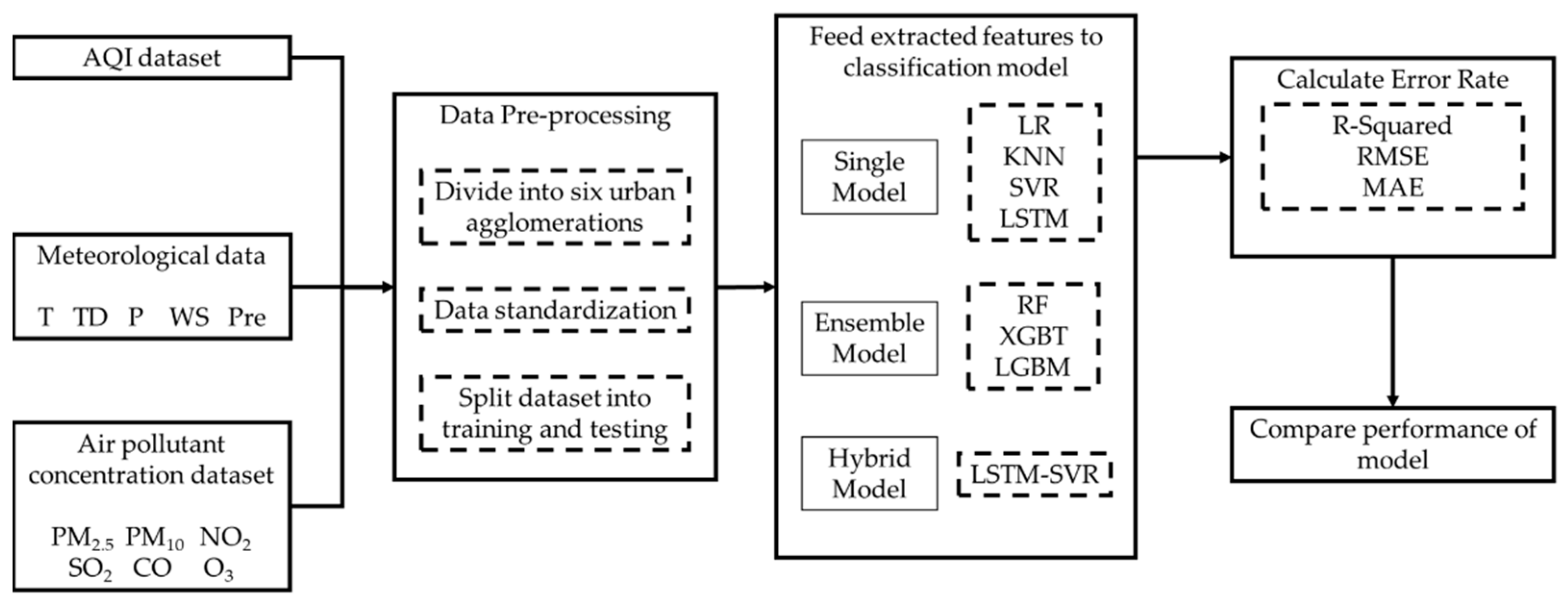
To overcome the above two challenges, this paper aims to realize the interregional comparison of the performance of models for air quality prediction and explore the differences between the three types of algorithmic models: he single model, the ensemble model, and the hybrid model. This research gathered daily mean Air Quality Index, air pollutant concentration data, and meteorological data from six major urban agglomerations in China, encompassing 95 cities, for the years 2017 to 2020. Subsequently, various models were developed, including Linear Regression (LR), K-Nearest Neighbor (KNN), Support Vector Regression (SVR), Long Short-Term Memory (LSTM) networks, ensemble models like Random Forest (RF), Extreme Gradient Boosting (XGBT), and Light Gradient Boosting Machine (LGBM). Additionally, considering prior research on single-model prediction, where the LSTM model was found to be suitable for time-series forecasting and widely applied in air quality prediction, and SVR displayed good performance in AQI prediction, being the optimal model in several studies [28,29], this paper further combined the independent SVR and LSTM models to construct an LSTM-SVR hybrid model. These models were employed to predict the Air Quality Index for six urban agglomerations in China, and the performance of the models in predicting different urban agglomerations was compared. Figure 1 presents the analytical framework of this paper.

3. Materials and Methods

3.1. Research Area

In recent years, to enhance the industrial linkage between various regions and develop economic clusters, urban agglomerations have gradually become an essential form of regional economic development in China. However, the spatial clustering effect of air pollution is also becoming more pronounced, and this is more apparent in urban agglomerations [41]. Simultaneously, the causes of air pollution exhibit heterogeneity across different cities in China [1], creating a complex environment for regional air quality prediction. This implies that models well-suited for predicting air quality in specific areas may only be applicable locally and not necessarily in other regions.

To comprehensively analyze the problem of air pollution and explore the general rules of differences in models for air quality prediction, urban agglomerations are an essential scale for studying the horizontal variations in model prediction performance. As shown in Figure 2, the research area of this paper is mainland China, six urban agglomerations have been selected, namely the Beijing–Tianjin–Hebei urban agglomeration (BTH-UA), Central Plains urban agglomeration (CP-UA), Yangtze River Delta urban agglomeration (YRD-UA), Middle Reaches of the Yangtze River urban agglomeration (YRMR-UA), Chengdu–Chongqing urban agglomeration (CY-UA), and Pearl River Delta urban agglomeration (PRD-UA).

3.2. Data Sources

This research used two sets of data, with a time dimension of the data samples from January 2017 to December 2020.

The first is data on air quality and air pollutant concentration, sourced from the real-time urban air quality publishing platform of China National Environmental Monitoring Center (CNEMC). The data include the AQI (Air Quality Index) and concentration indices of the six primary pollutants constituting the AQI assessment for 342 Chinese cities, namely PM_2.5, PM₁₀, CO, SO₂, NO₂, and O₃. The data are recorded on an hourly basis. The particulate matter, sulfur oxides, nitrogen oxides, and carbon monoxide generated by fossil fuel combustion and industrial activities are all classified as primary pollutants, and these primary pollutants undergo photochemical reactions to generate secondary pollutants such as ozone, causing diseases such as bronchitis and asthma [42]. Therefore, these six substances are the main sources of pollutants that cause changes in AQI [21], and many related studies have used these pollutants’ concentration data to predict AQI. The BA-LSSVM algorithm, constructed by Wu et al., considers air pollutant factors such as PM_2.5, PM₁₀, CO, SO₂, NO₂, and O₃ and takes predicted values from each component to obtain AQI predictions [16]. Senthil Kumar et al. not only used six types of pollutants but also added some nitrogen oxides and benzene pollutants to predict the environmental air quality index of cities in southern India [29]. In China’s air quality index composition system, the composition of AQI is determined based on the air quality sub-indices of these six pollutants. This study selects these six main pollutant concentration indices to participate in AQI prediction.

The second set consists of meteorological data obtained from the National Climatic Data Center (NCDC) in the United States, containing ground weather data for China. The data include information from nearly 400 meteorological monitoring stations and consist of five meteorological factors recorded every 3 h, including average temperature (T), pressure (P), dew point temperature (TD), wind speed (WS), and precipitation (Pre). Meteorology is an important factor that causes changes in air quality. Temperature and humidity can affect the chemical reactions of various pollutants [43]. Air pressure and wind can affect the diffusion and transportation of pollutants [44]. Precipitation has a washing and settling effect on pollutants and can further intensify the formation of secondary pollutants [45]. Meteorological factors and pollutant concentrations change dynamically. Related studies such as that of Sarkar et al. introduced four factors—temperature, humidity, solar radiation, and wind speed—combined with air pollutant factors to predict AQI [39]. Therefore, this article selects these five meteorological factors to construct a system for predicting AQI.

As the two sets of data were collected at different time intervals, the study converted the original hourly mean AQI and air pollutant concentration data and 3-hourly mean meteorological data into 24 h daily averages. This unification converted time series into daily fluctuations and linked the two sets of data.

Since the two data sets were collected at different geographic levels, with AQI and air pollutant concentration data at the city level and meteorological data at the level of the observation station, the study matched and integrated the meteorological data based on the cities where the observation stations were located. The study retained cities within the six major urban agglomerations, obtaining a collection of air quality and meteorological data for a total of 95 cities from 2017 to 2020. The final data indicators are presented in

Table 1. List of information on pollutant.

Variables	Symbol	Unit	Period	Source
Air Quality Index	AQI		January 2017–December 2020	China National Environmental Monitoring Center
Particulate Matter 2.5 µm	PM2.5	µg/m−3
Particulate Matter 10 µm	PM10	µg/m−3
Carbon Monoxide	CO	mg/m−3
Sulfur Dioxide	SO2	µg/m−3
Nitrogen Dioxide	NO2	µg/m−3
Ozone	O3	µg/m−3

and

Table 2. List of meteorological parameters.

Variables	Symbol	Unit	Period	Source
Air Temperature	T	°C	January 2017–December 2020	National Climatic Data Center
Atmospheric Pressure	P	hPa
Dew Temperature	TD	°C
Wind Speed	WS	m/s
Precipitation	Pre	mm

.

The count, mean, and standard deviation of the used data sets are shown in

Table 3. Information of pollutants and meteorological parameters.

	Count	Mean	Std
AQI	134,658	78.77	41.82
PM2.5	134,658	43.17	34.21
PM10	134,658	69.92	46.74
SO2	134,658	11.71	9.63
NO2	134,658	31.94	16.86
CO	134,658	0.85	0.43
O3	134,658	94.31	47.8
T	134,658	16.41	9.78
TD	134,658	10.26	11.18
P	134,658	1016.19	9.72
WS	134,658	2.49	1.41
Pre	134,658	3.94	14.21

. “Count” calculates the total number of non-missing values for each corresponding feature. “Mean” represents the average of all observed values. “Std” refers to the measurement of the dispersion of the data from the mean.

The monthly mean AQI and its maximum and minimum value distribution for the six urban agglomerations are presented in Figure 3. The calculations reveal that the Central Plains urban agglomeration (CP-UA) has the highest annual mean AQI, reaching 96.88, while the Pearl River Delta urban agglomeration (PRD-UA) has the lowest at 61.71. The annual mean AQIs are arranged in descending order as CP-UA, BTH-UA, YRD-UA, YRMR-UA, CY-UA, PRD-UA.

3.3. Machine Learning Models

This paper developed various machine learning models, ensemble models, and hybrid models and compared the results obtained from these models to evaluate the overall performance differences. This section will describe the basic information of using models.

3.3.1. Linear Regression (LR)

Linear Regression is the most commonly used machine learning method. It involves only one independent variable and explores the linear relationship between the independent variable (x) and the dependent variable (y). Linear Regression attempts to draw a line that best fits the points based on the given independent and dependent variables, minimizing the total error, and it is widely used in PM2.5 forecasting and various predictive-method comparative studies [34].

3.3.2. K-Nearest Neighbor (KNN)

In KNN, or the K-Nearest Neighbor method, a sample in KNN regression has K neighboring samples, and the weighted average value is assigned to this sample based on the characteristics of these neighboring samples, and then it generates a prediction [46]. In brief, it calculates the proximity of the K-nearest neighbor samples with the most similar features to a sample and chooses to operate according to the class with the highest frequency of occurrence [47].

For n-dimensional samples, the degree of closeness d can be expressed as

$$d=\sqrt{\sum _{i=1}^n{(a_i-b_i)}^2}$$

where a_i is the feature of the test set, b_i is the feature of the training set, and n is the number of features.

3.3.3. Support Vector Regression (SVR)

SVR (Support Vector Regression) is a use of SVM (Support Vector Machine) for regression problems. Support Vector Machine is a supervised learning method used for classification, regression, and outlier detection, which builds hyperplanes as boundaries between different data points, from which the output can be derived [30]. The SVR model creates a hyperplane on both sides of a linear function, with a spacing of $ϵ$, and does not calculate loss for all samples falling into the hyperplane. Only the support vectors will affect its functional model, finally obtaining the optimized model by minimizing the total loss and maximizing the margin.

The general Linear Regression SVR model function is

$$f\left(x\right)=W^T\phi \left(x\right)+b$$

where W is the weight vector, $b$ is the bias, and $\phi \left(x\right)$ is the high-dimensional feature space. The training and testing sets’ data are stored in the $\phi \left(x\right)$, which is nonlinearized and enters high-dimensional space. For the model function $+ϵ$ or $-ϵ$, it represents the upper and lower edges of the hyperplane. SVM can replace the vector’s inner product $\phi \left(x_i\right)·\phi \left(x_j\right)$ in high-dimensional space with the kernel function $K(x_i,x_j)$, which maps data to a high-dimensional feature space. It is widely used in small-sample-set predictions [48]. In this study, SVR uses the Gaussian Radial Basis Function (RBF) kernel, which is expressed as

$$K(x_i,x_j)=\exp (-\frac{{{\Vert x}_i-x_j\Vert }^2}{2{\sigma }^2})$$

where $\sigma$ is the bandwidth of the Gaussian kernel and $\mathrm{g}\mathrm{a}\mathrm{m}\mathrm{m}\mathrm{a}=1/2{\sigma }^2$. $\mathrm{G}\mathrm{a}\mathrm{m}\mathrm{m}\mathrm{a}$ is the parameter of the Gaussian radial basis kernel function.

3.3.4. Long Short-Term Memory (LSTM)

LSTM is a deep learning method, a variant of RNN. Compared to ordinary RNN, LSTM performs better in longer sequences, effectively solving the gradient explosion and vanishing problems generated by RNN [49], and it is widely used in time-series prediction. LSTM is divided into three stages internally, allowing control of information through the forget gate, the input gate, and the output gate. The output of the input gate is stored in the storage unit, gathering information received from the outside world; the forget gate provides instructions for what data need to be retained or discarded; and the output gate receives the calculation results. The specific model diagram is shown in Figure 4, where $i_t$ is the input gate, $f_t$ is the forget gate, $o_t$ is the output gate, $h_t$ is the output vector of the LSTM unit, $c_t$ represents the vector of the cell state, and $X_t$ is the input vector of the LSTM unit. $\sigma$ is each gate port, which information can be selectively passed through based on the nature of the gate.

3.3.5. Random Forest (RF)

Random Forest is a variant of the ensemble model Bagging. It is a supervised tree-based machine learning algorithm that can parallelly train independent decision tree (or forest) collections, and it is mostly used for multidimensional classification and regression problems [50]. Traditional decision trees choose an optimal feature from the current node’s feature set when selecting splitting features, while Random Forest uses decision trees as weak learners, enhancing model diversity by randomly selecting features on the basis of the random sampling of samples, for example, randomly selecting a subset containing k features from the feature set at each decision tree node and then selecting an optimal feature from this subset for splitting. According to the principle of averaging, the final model accuracy is estimated based on the average performance of all decision trees [51].

3.3.6. Extreme Gradient Boosting (XGBT)

XGBT, also known as XGBoost, is an ensemble model composed of K CART trees. It is an enhanced decision tree method that can create better learners based on model residuals, achieving distributed gradient boosting, and it can better control the complexity of the model. The objective function during XGBoost training consists of two parts: the first part is the loss of the gradient boosting algorithm, which can measure the difference between predicted values and actual values; the second part is the regularization term, defining the complexity of the model.

3.3.7. Light Gradient Boosting Machine (LGBM)

LGBM is widely known as LightGBM. Like XGBoost, it represents the ensemble method Boosting. Like XGBoost, LightGBM also uses decision trees as the base learner, but it provides faster training speed and lower memory usage. LightGBM uses Gradient One-sided Sampling (GOSS) to filter samples by deleting small gradient samples to reduce the quantity of samples. It employs Exclusive Feature Bundling (EFB) for the lossless merging of features, reducing the feature quantity, and further optimizing computation speed and memory usage.

3.3.8. LSTM-SVR

Utilizing a single model often does not yield satisfactory prediction results. To enhance prediction accuracy, this study combined the LSTM and SVR models, developing the LSTM-SVR hybrid model. This hybrid model aims to further correct the bias between the LSTM model’s predictions and the testing dataset by employing the SVR model with a Grid Search (GS) method.

The construction steps of the LSTM-SVR model are as follows:

• The previously set LSTM model was used to train and predict data for each urban agglomeration, resulting in a set of corresponding predictions y_pre.
• The D-value between the test dataset y_test and its corresponding predictions y_pre was calculated as e = y_test − y_pre.
• Using the SVR model on e, the Grid Search (GS) method was employed for predictions with the Gaussian Radial Basis Function (RBF) kernel. Then, the optimal penalty parameter C and the RBF kernel parameter gamma were obtained using the GS algorithm. The SVR model, equipped with these optimal parameters, was then used to predict the error e derived from the LSTM model, resulting in a corrected error $\overline{e}$.
• The predictions from the LSTM model y_pre were then combined with the error $\overline{e}$ corrections from SVR, obtaining the final prediction result ${\overline{y}}_{pre}=y_{pre}+\overline{e}$.

The schematic of the LSTM-SVR hybrid model is depicted in Figure 5.

Together with the hybrid model LSTM-SVR constructed using LSTM and SVR methods,

Table 4. AQI Prediction Models.

	Model
Single Model	LR
	KNN
	SVR
	LSTM
Ensemble Model	RF
	XGBT
	LGBM
Hybrid Model	LSTM-SVR

presents a total of 8 algorithms used in this paper, including single models, ensemble algorithm models, and hybrid algorithm models.

3.4. Model Performance Evaluation Metrics

Performance evaluation is one of the most critical steps in building models, and there are many metrics to assess the performance of a model. The evaluation metrics used in this work are R², MAE and RMSE.

3.4.1. R²

R², or R-squared, is the ratio of the regression sum of squares caused by variable x to the total sum of squares of y’s variation, also known as the coefficient of determination. It is very intuitive and easy to calculate in measuring the amount of variation in results.

3.4.2. MAE

Mean Absolute Error (MAE) adds the absolute difference between the actual output and predicted output of each observation in the entire dataset, then divides the resulting sum by the total number of observations. The purpose is to quantify the error in model prediction. Using the y test set’s output and prediction as an example, the formula is expressed as

$$MAE=\frac{1}{m}\sum _{i=1}^m|y_{test}^{\left(i\right)}-{\widehat{y}}_{test}^{\left(i\right)}|$$

3.4.3. RMSE

The Root Mean Squared Error (RMSE) is the square root of the Mean Squared Error (MSE). The MSE is the minimum absolute deviation between the observed actual output values and the model’s predicted values, represented by the average squared difference between the actual output and predicted output. The RMSE takes the square root of MSE, using the y test set output and prediction as an example, and the formula is expressed as

$$RMSE=\sqrt{\frac{1}{m}\sum _{i=1}^m(y_{test}^{\left(i\right)}-{\widehat{y}}_{test}^{\left(i\right)}){ }^2}$$

In the above expressions, $y_{test}^{\left(i\right)}$ serves as the actual output of the i-th sample in the y test set, ${\widehat{y}}_{test}^{\left(i\right)}$ is the predicted output of the i-th sample, and m is the total number of samples.

4. Implementation and Results of Data

The objective of this paper is to develop various types of prediction models that forecast the AQI values of urban agglomerations in China. While comparing the predictive capabilities of various models, a horizontal comparison of the model performance across different urban agglomerations was made, leading to a comprehensive evaluation of their predictive capabilities. This section further discusses the model configurations, implementation, and the results presented.

4.1. Data Preparation

The dataset of this study has the Air Quality Index (AQI) as its dependent variable, while the independent variables are composed of the concentration of six air pollutants and data on five meteorological factors.

Before determining the size of the training data set and the test data set, a careful evaluation was conducted in two ways to divide the training and testing data. The first method was to randomly divide the training and testing data proportionally, from 60% training set and 40% test set to 90% training set and 10% test set. Seven different proportional split methods were discussed, where the training and test set data were randomly selected. The second method was based on a time-series split, where 24:24 represents using data from 2017 to 2018 as the training set and data from 2019 to 2020 as the testing set; 36:12 indicates that the data from 2017 to 2019 would be used as the training set, and the data from 2020 would be used as the test set. The above two split methods will be discussed. The experiment used BTH-UA data to compare the scores of each model on different partitions of training and testing data. The results obtained are shown in

Table 5. Performance comparison based on the method of the training, validation, and testing split.

	Random Split				Time-Series Split
Model	60:40	70:30	80:20	90:10	24:24	36:12
LR	20.17	19.99	20.62	19.09	15.66	14.07
KNN	13.76	13.01	13.73	14.22	11.73	9.02
SVM	23.29	22.42	22.82	19.78	13.64	10.78
LSTM	13.47	13.12	13.65	11.84	9.28	6.98
RF	11.45	11.5	10.74	9.45	5.42	6.17
XGBT	8.91	9.23	8.25	7.64	6.95	6.57
LGBM	9.07	8.89	9.31	7.75	8.26	6.78
LSTM-SVR	12.56	12.53	12.95	11.2	5.09	3.28

. The results indicate that using time series to split the training and testing data sets can significantly improve the predictive performance of each model, especially in optimizing the performance of the hybrid model, LSTM-SVR. Among the time-series split set, the performance of 36:12 was the best.

Based on the above analysis and the empirical research on AQI time-series prediction, data from 2017 to 2019 were used as the training set, with a total of 100,754 single-day data packets used for AQI prediction training. Using the 2020 data as the test set, a total of 33,904 days of data were used to predict the AQI index. The ratio of training to testing was approximately 3:1. The size of the training and testing data for each urban agglomeration is shown in

Table 6. The size of training and testing data sets for different urban agglomerations.

	BTH-UA	CP-UA	YRD-UA	YRMR-UA	CY-UA	PRD-UA	SUM
Train_data	16,273	16,743	26,529	20,578	15,202	5429	100,754
Test_data	5470	5636	8930	6926	5114	1828	33,904
Test/Train	0.3361	0.3366	0.3366	0.3366	0.3364	0.3367	0.3365

. Different models were trained on the training dataset and the testing dataset was tested to evaluate the models’ performance.

Due to varying scales and magnitudes of data for different labels in the dataset, the standardization of training and testing data was essential to prevent significant fluctuations in prediction results and the overshadowing of vital features. We employed the Z-score method to subtract the mean from the data and scale it to unit variance, thus standardizing the features to a new dataset with a variance of 1 and a mean of 0. The mathematical representation is

$$X_{norm}=\frac{X-X_{mean}}{X_{std}}$$

where $X_{norm}$ represents the standardized value, $X_{mean}$ is the overall mean, and $X_{std}$ is the standard deviation of the data.

4.2. Model Parameter Tuning

In this study, we constructed eight models, LR, KNN, SVR, LSTM, RF, XGBT, LGBM, and LSTM-SVR, to predict the air quality index of urban agglomerations. In order to obtain the optimal parameters of each model, the Grid Search method (GS) was used to optimize the hyperparameters of each model. During the tuning process, a total dataset of all urban agglomerations was used to participate in training, with 100,754 training data and 33,904 test data. The validation set was subjected to five-fold cross-validation to determine the optimal parameters. The final determined model hyperparameters are shown in

Table 7. Summary of parameter values in each model.

Model	Parameter	Determined Value
LR	penalty	L2
	tol	0.0001
KNN	n_neighbors	5
	weights	uniform
	algorithm	auto
SVR	kernel	RBF
	gamma	0.1
	C	10
LSTM	time_steps	1
	input layer neurons	11
	hidden layers	2
	hidden layer neurons	64
	hidden layer activation	Relu
	output layer neurons	1
	epochs	10
	batch_size	16
	validation_split	0.2
RF	n_estimators	150
	max_depth	30
	min_samples_split	4
	min_samples_leaf	2
XGBT	learning rate	0.1
	n_estimators	1250
	max_depth	8
	min_child_weight	11
	gamma	0.8
	subsample	0.9
	colsample_bytree	0.8
	reg_alpha	0.05
LGBM	learning_rate	0.3
	n_estimators	1500
	max_depth	4
	feature_fraction	0.9
	bagging_fraction	0.6
	lambda	0.2
	num leaves	8
	min split gain	0.0

.

The data preparation for the six urban agglomerations was performed separately, with models trained to predict the AQI. The performance evaluations were performed using the R², RMSE, and MAE methods, and the detailed results are presented in

Table 8. Prediction Accuracy (R²) of AQI predictions using eight models for the six major urban agglomerations.

	BTH-UA	CP-UA	YRD-UA	YRMR-UA	CY-UA	PRD-UA	Mean-ML
LR	0.888	0.822	0.835	0.889	0.845	0.880	0.860
KNN	0.954	0.938	0.950	0.948	0.944	0.941	0.946
SVR	0.934	0.901	0.945	0.940	0.929	0.931	0.930
LSTM	0.972	0.945	0.981	0.988	0.991	0.986	0.977
RF	0.982	0.960	0.994	0.997	0.999	0.999	0.989
XGBT	0.980	0.963	0.993	0.996	0.998	0.995	0.988
LGBM	0.974	0.960	0.990	0.995	0.997	0.996	0.985
LSTM-SVR	0.994	0.981	0.994	0.997	0.998	0.996	0.993
Mean-UA	0.960	0.934	0.960	0.969	0.963	0.966	0.958

,

Table 9. Prediction accuracy (RMSE) of AQI predictions using eight models for the six major urban agglomerations.

	BTH-UA	CP-UA	YRD-UA	YRMR-UA	CY-UA	PRD-UA	Mean-ML
LR	14.067	17.229	11.626	10.166	11.625	9.409	12.354
KNN	9.024	10.204	6.389	7.840	6.998	6.591	7.841
SVR	10.782	12.890	6.721	7.507	7.842	7.148	8.815
LSTM	6.976	9.557	3.955	3.408	2.813	3.242	4.992
RF	5.641	8.169	2.203	1.571	1.029	0.715	3.221
XGBT	5.935	7.841	2.388	1.862	1.374	1.969	3.562
LGBM	6.749	8.186	2.808	2.145	1.628	1.760	3.879
LSTM-SVR	3.277	5.667	2.255	1.765	1.444	1.633	2.674
Mean-UA	7.806	9.968	4.793	4.533	4.344	4.058	5.917

and

Table 10. Prediction accuracy (MAE) of AQI predictions using eight models for the six major urban agglomerations.

	BTH-UA	CP-UA	YRD-UA	YRMR-UA	CY-UA	PRD-UA	Mean-ML
LR	10.547	12.906	8.821	7.840	8.656	6.715	9.248
KNN	5.795	6.042	4.477	4.976	4.899	4.609	5.133
SVR	4.936	5.912	3.301	3.694	3.778	4.297	4.320
LSTM	4.497	4.591	2.656	2.567	2.101	2.446	3.143
RF	0.918	0.913	0.659	0.560	0.422	0.359	0.638
XGBT	1.877	2.027	1.179	1.096	0.950	1.425	1.426
LGBM	2.519	2.379	1.436	1.236	1.064	1.220	1.642
LSTM-SVR	1.754	1.851	1.123	1.077	0.910	1.042	1.293
Mean-UA	4.105	4.578	2.957	2.881	2.848	2.764	3.355

To offer a more direct comparison of model performance across different urban agglomerations, performance evaluations for the three metrics were plotted as line graphs, as shown in Figure 6, Figure 7 and Figure 8. In the tables, to compare the predictive abilities of the eight models, we calculated the average R², RMSE, and MAE values for each model’s predictions across all urban agglomerations, represented as Mean-ML. In comparing the differences in predictive performance across urban agglomerations, we calculated the average R², RMSE, and MAE values for the six urban agglomerations, as predicted by all the models, represented as Mean-UA.

The training time of each model is shown in Table 8, with LR and KNN having the shortest time. Among the ensemble models, XGBT has the longest time, and LGBM has the shortest time. The hybrid model LSTM-SVR includes Grid Search steps, LSTM, and SVR model predictions, so it has the longest time among all the models.

4.3. Performance of Single Models

The single-model prediction focused on the prediction of urban agglomeration AQI using four methods: LR, KNN, SVR, and LSTM. During the application of the KNN algorithm, a K-Nearest Neighbors model with five neighbors was used for predictions. For SVR, the commonly used Gaussian Radial Basis Function (RBF) kernel parameter was employed to construct a Support Vector Machine model for the training dataset, enhancing its non-linearity. When constructing the LSTM model, to solely rely on the air pollution concentration and meteorological conditions for predicting the AQI in a day, the time-step length of the input layer was set to 1, and all 11 feature vectors were input to the input layer. Two hidden layers were then built, each containing 64 neurons, and the “Relu” activation function was applied. The output layer had one target neuron. To improve the efficiency of model training, the batch size and epoch for the LSTM model were set to 16 and 10, respectively. The final prediction results are presented in Table 8, Table 9 and Table 10. The R² values, in descending order, are LSTM, KNN, SVR, and LR. The RMSE values, from best to worst, are LSTM, KNN, SVR, and LR. MAE values, from the best to worst, are LSTM, SVR, KNN, and LR.

4.4. Performance of Ensemble Learning Models

The ensemble algorithm used LR, XGBT, and LGBM to predict the urban agglomerations’ AQI. The final prediction results are presented in Table 8, Table 9 and Table 10. The R² values, in descending order, are RF, XGBT, and LGBM. The RMSE values and MAE values, from best to worst, are RF, LGBM, and XGBT. Overall, RF has the best comprehensive performance. Next is XGBT, but in the ensemble models, XGBT takes the longest time. LGBM has the worst performance with the shortest training time, and its RMSE and MAE are better than XGBT in predicting PRD-UA.

4.5. Performance of Hybrid Learning Model LSTM-SVR

Table 9 displays the optimal penalty parameter C and the RBF kernel parameter $\mathrm{g}\mathrm{a}\mathrm{m}\mathrm{m}\mathrm{a}$ for each urban agglomeration, determined through the GS algorithm. All urban agglomerations had identical optimal values for C and gamma, namely 10 and 0.1, respectively. The final ${\overline{y}}_{pre}$ predictions were evaluated using the R², RMSE, and MAE metrics, determining the model’s predictive capabilities. As shown in Table 10,

Table 11. Model training time for different urban agglomerations.

	Model Training Time (s)
	BTH-UA	CP-UA	YRD-UA	YRMR-UA	CY-UA	PRD-UA
LR	0.203	0.005	0.006	0.016	0.006	0.001
KNN	0.232	0.177	0.057	0.047	0.040	0.219
SVR	10.727	12.939	31.614	20.362	9.364	1.328
LSTM	21.774	23.931	32.610	24.317	23.082	9.723
RF	15.913	13.752	21.065	18.615	11.552	4.423
XGBT	21.991	22.832	26.711	22.223	17.086	13.292
LGBM	8.220	7.140	2.569	3.985	2.157	7.327
LSTM-SVR	160.332	237.714	547.042	327.92	180.53	31.512

and

Table 12. SVR model parameters obtained from Grid Search (GS).

	BTH-UA	CP-UA	YRD-UA	YRMR-UA	CY-UA	PRD-UA
C	10	10	10	10	10	10
gamma	0.1	0.1	0.1	0.1	0.1	0.1

, compared to other models, the LSTM-SVR model showed superior R² and RMSE, as well as the second-best ranked MAE.

4.6. Taylor Diagram Graphical Presentation for Models

To provide a more comprehensive presentation, we used the graphical presentation of the Taylor diagram [25] to test all prediction models, as shown in Figure 9. The Taylor diagram can summarize the degree of matching between the model predictions and the observation results and helps to understand the performance of models. It provides the correlation coefficient and normalized standard deviation of each model, and the distance from the observation point is the ratio of the standard deviation of the model’s predictions to the standard deviation of the observations. The closer the distance is to 1, the greater the prediction accuracy. The scale of the outer chord of the circle represents the correlation coefficient, and the shorter the vertical distance between the model and the X-axis, the higher the correlation coefficient.

Therefore, the position of each model symbol appearing in the chart quantifies the degree of matching between the predicted AQI of the model and the observed values, and the predictive performance of the model can be seen. It can be seen that LSTM-SVR performs better than all the other models in predicting BTH-UA and CP-UA. In the prediction of CY-UA and PRD-UA, RF performs better than LSTM-SVR. The overall prediction accuracy of a single model is not as good as that of ensemble models and hybrid models.

5. Discussion

This section discusses the comparative predictive performance of eight models for AQI prediction in six urban agglomerations. The predictive accuracy of the algorithm in each urban agglomeration was obtained based on R², RMSE, and MAE, comparing the predictive performance between machine learning models and the predictive accuracy among urban agglomerations.

In the comparison of predictive accuracy among urban agglomerations, the Mean-UA levels of RMSE and MAE are arranged in order from poor to good, according to the order of CP-UA, BTH-UA, YRD-UA, YMRM-UA, CY-UA, and PRD-UA. CP-UA has the worst overall predictive accuracy among all urban agglomerations, while PRD-UA has the best predictive accuracy. This may be related to the level of air pollution in the urban agglomerations, as CP-UA and PRD-UA are the areas with the highest and lowest annual average AQI index, respectively. Previous studies have shown that prediction accuracy in China’s northern regions, where air pollution is severe, will significantly decrease due to the more diverse and complex factors causing the increase in various air pollutants [52]. In the comparison of Figure 6, Figure 7 and Figure 8, it can be found that single models have significant differences in predictive performance in different urban agglomerations, while the differences in performance in ensemble learning models are smaller. A few algorithms with higher predictive accuracy easily coincide in their performance curves on YRMR-UA, CY-UA, and PRD-UA, and there is a noticeable gap in BTH-UA, CP-UA, and YRD-UA. With the best predictive performance, the LSTM and RF models further narrow the differences in predictive performance among urban agglomerations, making the predictive performance curves more even. This indicates that the best-performing LSTM-SVR and RF can further reduce the differences in predictive accuracy among different urban agglomerations, further enhance the predictive performance in areas with serious air pollution like BTH-UA, CP-UA, and YRD-UA, and solve the problem of low prediction accuracy in areas with severe pollution.

In the comparison of predictive performance among eight different algorithmic models, based on the Mean-ML of R², RMSE, and MAE, the simplest LR model has the worst predictive performance, the LSTM model has the best performance in single models, and SVR and KNN perform similarly. Ensemble algorithm models generally perform significantly better than single models. Among them, RF has the best predictive performance, where R², RMSE, and MAE are all better than those from the other two algorithms, and it obtained the best MAE value. XGBT is generally superior to LGBM, but LGBM also has the advantage of low time consumption. The hybrid model algorithm LSTM-SVR that we constructed obtained the best R² and RMSE among the developed models and was only slightly worse than RF on MAE. Compared to RF, LSTM-SVR significantly reduced the RMSE values in the heavily polluted BTH-UA and CP-UA regions, while the RMSE values obtained in predicting YRD-UA, YRMR-UA, CY-UA, and PRD-UA were all worse than RF. The LSTM-SVR model has a good effect on enhancing the accuracy of AQI prediction in high-pollution areas. LSTM-SVR’s performance is also far better than the LSTM model. This indicates that the constructed LSTM-SVR hybrid model has significant predictive advantages compared to single models and some ensemble models, providing an effective method for regional air quality prediction, and the hybrid model prediction has further development prospects [53].

6. Conclusions

Currently, with the development of industry and cities, the intensification of air pollution, and the increasingly complex situation faced by air quality monitoring and forecasting, the pursuit of accurate, efficient, and stable air quality prediction is of great importance for environmental governance and sustainable development.

Considering pollution source information and meteorological data to simulate air quality is widely used in most studies [54,55]. This study utilized air pollutant concentration and meteorological data from 2017 to 2020 in six Chinese urban agglomerations to simulate air quality conditions [56]. To predict air quality, this study employed seven single models and ensemble models of machine learning methods and constructed a hybrid LSTM-SVR model to predict air quality in the six urban agglomerations. Using R², RMSE, and MAE as evaluation metrics, a comprehensive comparison of the predictive performance of eight algorithm models was made from the perspectives of differences in models and differences in urban agglomerations [57].

The results show that in areas where air pollution is more severe, the situation faced by the model prediction is more complex, and the prediction accuracy has decreased. The more accurate RF and LSTM-SVR models can effectively improve the prediction accuracy of air quality in areas with severe air pollution. Comparing the overall performance of eight prediction models, the constructed hybrid model LSTM-SVR achieved the best R² and RMSE; the ensemble model RF obtained the best MAE; and XGBT and LGBM were also noteworthy in their predictive effects. These results also confirmed that hybrid models and ensemble models are generally superior to prediction methods using single models [58,59], and LSTM-SVR has been proven to be a reliable method for predicting AQI. This contributes to the practical application of air pollution control and promotes ecological governance and green development in China [60].

This study also has many shortcomings. First, the research only considered meteorological conditions and the concentration of air pollutants in predicting the air quality index, and since the data time series is measured daily, some factors that are difficult to calculate as daily averages but are well-studied, such as population elements, economic activities, and geographical environment, were not considered in the model analysis. Second, the data from different sites in each urban agglomeration did not form effective clusters in the research, and each site was an independent time-series data set, resulting in fragmented time-series data being fed into the model, which could have caused some prediction interference. Third, the model algorithms compared in the study were not comprehensive enough, such as the lack of comparison with the performance of the stacking model in ensemble learning. Fourth, this study only explored the predictive performance of different models and did not further delve into measuring the feature importance of AQI using high-performing models, performing feature selection, or constructing new features. So this article only provides a better model-selection perspective in AQI prediction, but there is not much discussion on analyzing the causes that affect the quality of AQI and providing decision-making opinions for specific pollutant treatment. In subsequent research, we will further overcome these shortcomings and improve the depth and breadth of the application of artificial intelligence technology in air quality prediction.

References

1. Zhan, D.; Kwan, M.-P.; Zhang, W.; Yu, X.; Meng, B.; Liu, Q. The Driving Factors of Air Quality Index in China. J. Cleaner Production 2018, 197, 1342–1351. [Google Scholar] [CrossRef]
2. Jo, S.; Kim, Y.-J.; Park, K.W.; Hwang, Y.S.; Lee, S.H.; Kim, B.J.; Chung, S.J. Association of NO2 and Other Air Pollution Exposures with the Risk of Parkinson Disease. JAMA Neurol. 2021, 78, 800. [Google Scholar] [CrossRef] [PubMed]
3. Zhao, S.; Liu, S.; Hou, X.; Sun, Y.; Beazley, R. Air Pollution and Cause-Specific Mortality: A Comparative Study of Urban and Rural Areas in China. Chemosphere 2021, 262, 127884. [Google Scholar] [CrossRef]
4. Hoq, M.N.; Alam, R.; Amin, A. Prediction of Possible Asthma Attack from Air Pollutants: Towards a High Density Air Pollution Map for Smart Cities to Improve Living. In Proceedings of the 2019 International Conference on Electrical, Computer and Communication Engineering (ECCE), Cox’s Bazar, Bangladesh, 7–9 February 2019; pp. 1–5. [Google Scholar]
5. Maciejczyk, P.; Chen, L.-C.; Thurston, G. The Role of Fossil Fuel Combustion Metals in PM2.5 Air Pollution Health Associations. Atmosphere 2021, 12, 1086. [Google Scholar] [CrossRef]
6. Dominski, F.H.; Lorenzetti Branco, J.H.; Buonanno, G.; Stabile, L.; Gameiro Da Silva, M.; Andrade, A. Effects of Air Pollution on Health: A Mapping Review of Systematic Reviews and Meta-Analyses. Environ. Res. 2021, 201, 111487. [Google Scholar] [CrossRef] [PubMed]
7. Zhan, Y.; Luo, Y.; Deng, X.; Chen, H.; Grieneisen, M.L.; Shen, X.; Zhu, L.; Zhang, M. Spatiotemporal Prediction of Continuous Daily PM2.5 Concentrations across China Using a Spatially Explicit Machine Learning Algorithm. Atmos. Environ. 2017, 155, 129–139. [Google Scholar] [CrossRef]
8. Franklin, B.A.; Brook, R.; Arden Pope, C. Air Pollution and Cardiovascular Disease. Curr. Probl. Cardiol. 2015, 40, 207–238. [Google Scholar] [CrossRef]
9. Pandey, A.; Brauer, M.; Cropper, M.L.; Balakrishnan, K.; Mathur, P.; Dey, S.; Turkgulu, B.; Kumar, G.A.; Khare, M.; Beig, G.; et al. Health and Economic Impact of Air Pollution in the States of India: The Global Burden of Disease Study 2019. Lancet Planet. Health 2021, 5, e25–e38. [Google Scholar] [CrossRef]
10. Burnett, R.; Chen, H.; Szyszkowicz, M.; Fann, N.; Hubbell, B.; Pope, C.A.; Apte, J.S.; Brauer, M.; Cohen, A.; Weichenthal, S.; et al. Global Estimates of Mortality Associated with Long-Term Exposure to Outdoor Fine Particulate Matter. Proc. Natl. Acad. Sci. USA 2018, 115, 9592–9597. [Google Scholar] [CrossRef]
11. Aryal, A.; Harmon, A.C.; Dugas, T.R. Particulate Matter Air Pollutants and Cardiovascular Disease: Strategies for Intervention. Pharmacol. Ther. 2021, 223, 107890. [Google Scholar] [CrossRef]
12. Wang, J.; Li, J.; Wang, X.; Wang, J.; Huang, M. Air Quality Prediction Using CT-LSTM. Neural Comput. Appl. 2021, 33, 4779–4792. [Google Scholar] [CrossRef]
13. Madan, T.; Sagar, S.; Virmani, D. Air Quality Prediction Using Machine Learning Algorithms–A Review. In Proceedings of the 2020 2nd International Conference on Advances in Computing, Communication Control and Networking (ICACCCN), Greater Noida, India, 18–19 December 2020; pp. 140–145. [Google Scholar]
14. Wang, J.; Zhang, X.; Guo, Z.; Lu, H. Developing an Early-Warning System for Air Quality Prediction and Assessment of Cities in China. Expert Syst. Appl. 2017, 84, 102–116. [Google Scholar] [CrossRef]
15. Li, Y.; Chiu, Y.; Lu, L.C. Energy and AQI Performance of 31 Cities in China. Energy Policy 2018, 122, 194–202. [Google Scholar] [CrossRef]
16. Wu, Q.; Lin, H. A Novel Optimal-Hybrid Model for Daily Air Quality Index Prediction Considering Air Pollutant Factors. Sci. Total Environ. 2019, 683, 808–821. [Google Scholar] [CrossRef]
17. Ji, C.; Zhang, C.; Hua, L.; Ma, H.; Nazir, M.S.; Peng, T. A Multi-Scale Evolutionary Deep Learning Model Based on CEEMDAN, Improved Whale Optimization Algorithm, Regularized Extreme Learning Machine and LSTM for AQI Prediction. Environ. Res. 2022, 215, 114228. [Google Scholar] [CrossRef]
18. Liu, X.; Guo, H. Air Quality Indicators and AQI Prediction Coupling Long-Short Term Memory (LSTM) and Sparrow Search Algorithm (SSA): A Case Study of Shanghai. Atmos. Pollut. Res. 2022, 13, 101551. [Google Scholar] [CrossRef]
19. Liu, H.; Zhang, X. AQI Time Series Prediction Based on a Hybrid Data Decomposition and Echo State Networks. Environ. Sci. Pollut. Res. 2021, 28, 51160–51182. [Google Scholar] [CrossRef]
20. Masih, A. Machine Learning Algorithms in Air Quality Modeling. Global J. Environ. Sci. Manag. 2019, 5, 515–534. [Google Scholar] [CrossRef]
21. Balogun, A.-L.; Tella, A.; Baloo, L.; Adebisi, N. A Review of the Inter-Correlation of Climate Change, Air Pollution and Urban Sustainability Using Novel Machine Learning Algorithms and Spatial Information Science. Urban Clim. 2021, 40, 100989. [Google Scholar] [CrossRef]
22. Rybarczyk, Y.; Zalakeviciute, R. Machine Learning Approaches for Outdoor Air Quality Modelling: A Systematic Review. Appl. Sci. 2018, 8, 2570. [Google Scholar] [CrossRef]
23. Spinelle, L.; Gerboles, M.; Villani, M.G.; Aleixandre, M.; Bonavitacola, F. Field Calibration of a Cluster of Low-Cost Available Sensors for Air Quality Monitoring. Part A: Ozone and Nitrogen Dioxide. Sens. Actuators B Chem. 2015, 215, 249–257. [Google Scholar] [CrossRef]
24. Baran, B. Air Quality Index Prediction in Besiktas District by Artificial Neural Networks and K Nearest Neighbors. Mühendislik Bilim. Tasarım Derg. 2021, 9, 52–63. [Google Scholar] [CrossRef]
25. Liu, B.-C.; Binaykia, A.; Chang, P.-C.; Tiwari, M.K.; Tsao, C.-C. Urban Air Quality Forecasting Based on Multi-Dimensional Collaborative Support Vector Regression (SVR): A Case Study of Beijing-Tianjin-Shijiazhuang. PLoS ONE 2017, 12, e0179763. [Google Scholar] [CrossRef] [PubMed]
26. Yan, R.; Liao, J.; Yang, J.; Sun, W.; Nong, M.; Li, F. Multi-Hour and Multi-Site Air Quality Index Forecasting in Beijing Using CNN, LSTM, CNN-LSTM, and Spatiotemporal Clustering. Expert Syst. Appl. 2021, 169, 114513. [Google Scholar] [CrossRef]
27. Ketu, S. Spatial Air Quality Index and Air Pollutant Concentration Prediction Using Linear Regression Based Recursive Feature Elimination with Random Forest Regression (RFERF): A Case Study in India. Nat. Hazards 2022, 114, 2109–2138. [Google Scholar] [CrossRef]
28. Pan, B. Application of XGBoost Algorithm in Hourly PM2.5 Concentration Prediction. IOP Conf. Ser. Earth Environ. Sci. 2018, 113, 012127. [Google Scholar] [CrossRef]
29. Kumar, R.S.; Arulanandham, A.; Arumugam, S.; Dinesh, G.; Thirukkumaran, R.; Subashmoorthy, R. Analysis of Classification and Clustering Techniques for Ambient AQI Using Machine Learning Algorithms. In Proceedings of the 2022 4th International Conference on Smart Systems and Inventive Technology (ICSSIT), Tirunelveli, India, 20–22 January 2022; pp. 902–908. [Google Scholar]
30. Liang, Y.-C.; Maimury, Y.; Chen, A.H.-L.; Juarez, J.R.C. Machine Learning-Based Prediction of Air Quality. Appl. Sci. 2020, 10, 9151. [Google Scholar] [CrossRef]
31. Li, S.; Paoli, R. Comparison of Machine Learning Models for Data-Driven Aircraft Icing Severity Evaluation. J. Aerosp. Inf. Syst. 2021, 18, 973–977. [Google Scholar] [CrossRef]
32. Ren, L.; Matsumoto, K. Effects of Socioeconomic and Natural Factors on Air Pollution in China: A Spatial Panel Data Analysis. Sci. Total Environ. 2020, 740, 140155. [Google Scholar] [CrossRef]
33. Janarthanan, R.; Partheeban, P.; Somasundaram, K.; Navin Elamparithi, P. A Deep Learning Approach for Prediction of Air Quality Index in a Metropolitan City. Sustain. Cities Soc. 2021, 67, 102720. [Google Scholar] [CrossRef]
34. Liu, H.; Fang, C.; Zhang, X.; Wang, Z.; Bao, C.; Li, F. The Effect of Natural and Anthropogenic Factors on Haze Pollution in Chinese Cities: A Spatial Econometrics Approach. J. Clean. Prod. 2017, 165, 323–333. [Google Scholar] [CrossRef]
35. Castelli, M.; Clemente, F.M.; Popovič, A.; Silva, S.; Vanneschi, L. A Machine Learning Approach to Predict Air Quality in California. Complexity 2020, 2020, 8049504. [Google Scholar] [CrossRef]
36. Liu, H.; Li, Q.; Yu, D.; Gu, Y. Air Quality Index and Air Pollutant Concentration Prediction Based on Machine Learning Algorithms. Appl. Sci. 2019, 9, 4069. [Google Scholar] [CrossRef]
37. Li, W.; Kang, S.; Sun, Y.; Bai, W.; Wang, Y.; Song, H. A Machine Learning Approach for Air-Quality Forecast by Integrating GNSS Radio Occultation Observation and Weather Modeling. Atmosphere 2022, 14, 58. [Google Scholar] [CrossRef]
38. Sarkar, N.; Gupta, R.; Keserwani, P.K.; Govil, M.C. Air Quality Index Prediction Using an Effective Hybrid Deep Learning Model. Environ. Pollut. 2022, 315, 120404. [Google Scholar] [CrossRef]
39. Zhang, Z.; Zeng, Y.; Yan, K. A Hybrid Deep Learning Technology for PM2.5 Air Quality Forecasting. Environ. Sci. Pollut. Res. 2021, 28, 39409–39422. [Google Scholar] [CrossRef] [PubMed]
40. Mao, W.; Wang, W.; Jiao, L.; Zhao, S.; Liu, A. Modeling Air Quality Prediction Using a Deep Learning Approach: Method Optimization and Evaluation. Sustain. Cities Soc. 2021, 65, 102567. [Google Scholar] [CrossRef]
41. Luo, H.; Han, Y.; Cheng, X.; Lu, C.; Wu, Y. Spatiotemporal Variations in Particulate Matter and Air Quality over China: National, Regional and Urban Scales. Atmosphere 2020, 12, 43. [Google Scholar] [CrossRef]
42. Wang, L.; Wang, J.; Tan, X.; Fang, C. Analysis of NOx Pollution Characteristics in the Atmospheric Environment in Changchun City. Atmosphere 2019, 11, 30. [Google Scholar] [CrossRef]
43. Largeron, Y.; Staquet, C. Persistent Inversion Dynamics and Wintertime PM10 Air Pollution in Alpine Valleys. Atmos. Environ. 2016, 135, 92–108. [Google Scholar] [CrossRef]
44. Monteiro, A.; Gama, C.; Cândido, M.; Ribeiro, I.; Carvalho, D.; Lopes, M. Investigating Ozone High Levels and the Role of Sea Breeze on Its Transport. Atmos. Pollut. Res. 2016, 7, 339–347. [Google Scholar] [CrossRef]
45. Chen, Z.; Xie, X.; Cai, J.; Chen, D.; Gao, B.; He, B.; Cheng, N.; Xu, B. Understanding Meteorological Influences on PM 2.5 Concentrations across China: A Temporal and Spatial Perspective. Atmos. Chem. Phys. 2018, 18, 5343–5358. [Google Scholar] [CrossRef]
46. Kumar, V.; Sahu, M. Evaluation of Nine Machine Learning Regression Algorithms for Calibration of Low-Cost PM2.5 Sensor. J. Aerosol Sci. 2021, 157, 105809. [Google Scholar] [CrossRef]
47. Danesh Yazdi, M.; Kuang, Z.; Dimakopoulou, K.; Barratt, B.; Suel, E.; Amini, H.; Lyapustin, A.; Katsouyanni, K.; Schwartz, J. Predicting Fine Particulate Matter (PM2.5) in the Greater London Area: An Ensemble Approach Using Machine Learning Methods. Remote Sens. 2020, 12, 914. [Google Scholar] [CrossRef]
48. Zhao, Z.; Wu, J.; Cai, F.; Zhang, S.; Wang, Y.-G. A Statistical Learning Framework for Spatial-Temporal Feature Selection and Application to Air Quality Index Forecasting. Ecol. Indic. 2022, 144, 109416. [Google Scholar] [CrossRef]
49. Liu, X.; Li, W. MGC-LSTM: A Deep Learning Model Based on Graph Convolution of Multiple Graphs for PM2.5 Prediction. Int. J. Environ. Sci. Technol. 2023, 20, 10297–10312. [Google Scholar] [CrossRef]
50. Lee, Y.S.; Choi, E.; Park, M.; Jo, H.; Park, M.; Nam, E.; Kim, D.G.; Yi, S.-M.; Kim, J.Y. Feature Extraction and Prediction of Fine Particulate Matter (PM2.5) Chemical Constituents Using Four Machine Learning Models. Expert Syst. Appl. 2023, 221, 119696. [Google Scholar] [CrossRef]
51. Schneider, R.; Vicedo-Cabrera, A.; Sera, F.; Masselot, P.; Stafoggia, M.; De Hoogh, K.; Kloog, I.; Reis, S.; Vieno, M.; Gasparrini, A. A Satellite-Based Spatio-Temporal Machine Learning Model to Reconstruct Daily PM2.5 Concentrations across Great Britain. Remote Sens. 2020, 12, 3803. [Google Scholar] [CrossRef]
52. Zhu, S.; Yang, L.; Wang, W.; Liu, X.; Lu, M.; Shen, X. Optimal-Combined Model for Air Quality Index Forecasting: 5 Cities in North China. Environ. Pollut. 2018, 243, 842–850. [Google Scholar] [CrossRef]
53. Wang, J.; Li, X.; Jin, L.; Li, J.; Sun, Q.; Wang, H. An Air Quality Index Prediction Model Based on CNN-ILSTM. Sci. Rep. 2022, 12, 8373. [Google Scholar] [CrossRef]
54. Kadiyala, A.; Kumar, A. Guidelines for Operational Evaluation of Air Quality Models; Lambert Academic Publishing GmbH & Co.: Saarland, Germany, 2012; p. 123. [Google Scholar]
55. Madiraju, S.V.H.; Kumar, A. Development and Evaluation of SLINE 1.0, a Line Source Dispersion Model for Gaseous Pollutants by Incorporating Wind Shear Near the Ground under Stable and Unstable Atmospheric Conditions. Atmosphere 2021, 12, 618. [Google Scholar] [CrossRef]
56. Nimmatoori, P.; Kumar, A. Dispersion Modeling of Particulate Matter in Different Size Ranges Releasing from a Biosolids Applied Agricultural Field Using Computational Fluid Dynamics. Adv. Chem. Eng. Sci. 2021, 11, 180–202. [Google Scholar] [CrossRef]
57. Riswadkar, R.M.; Kumar, A. Evaluation of the Industrial Source Complex Short-Term Model in a Large-Scale Multiple Source Region for Different Stability Classes. Environ. Monit. Assess. 1994, 33, 19–32. [Google Scholar] [CrossRef] [PubMed]
58. Zhu, S.; Lian, X.; Liu, H.; Hu, J.; Wang, Y.; Che, J. Daily Air Quality Index Forecasting with Hybrid Models: A Case in China. Environ. Pollut. 2017, 231, 1232–1244. [Google Scholar] [CrossRef] [PubMed]
59. Zhan, C.; Jiang, W.; Lin, F.; Zhang, S.; Li, B. A Decomposition-Ensemble Broad Learning System for AQI Forecasting. Neural Comput. Appl. 2022, 34, 18461–18472. [Google Scholar] [CrossRef]
60. Zhang, B.; Mei, Y. Rural Ecological Environment Governance in the Context of Rural Revitalization: Policy Evolution and Path Selection. J. Nanjing Agric. Univ. 2023, 23, 112–120. [Google Scholar] [CrossRef]
Figure 1. The research framework.
Atmosphere 14 01478 g001
Figure 2. Distribution of six major urban agglomerations in China.
Atmosphere 14 01478 g002
Figure 3. Monthly variation in AQI in China’s six major urban agglomerations: the median (central horizontal line within the box), 25th and 75th percentiles (lower and upper bars within the boxes, respectively), minimum and maximum (lowest horizontal line and highest point, respectively) are shown.
Atmosphere 14 01478 g003
Figure 4. The network structure of the LSTM.
Atmosphere 14 01478 g004
Figure 5. Schematic diagram of the LSTM-SVR combination model.
Atmosphere 14 01478 g005
Figure 6. Prediction accuracy (R2) line chart of AQI prediction.
Atmosphere 14 01478 g006
Figure 7. Prediction accuracy (RMSE) line chart of AQI prediction.
Atmosphere 14 01478 g007
Figure 8. Prediction accuracy (MAE) line chart of AQI prediction.
Atmosphere 14 01478 g008
Figure 9. Taylor diagram graphical presentation for the eight predictive models, including LR, KNN, SVR, LSTM, RF, XGBT, LGBM, and LSTM-SVR. The red line represents the normalized standard deviation ratio between the predicted and observed values of the model. The green line represents the correlation coefficient of the model. The semicircular blue line is an auxiliary line used to display the distance between the model and the optimal performance point REF (The normalization coefficient of predicted and observed values is 1, and the model correlation coefficient is 1).
Atmosphere 14 01478 g009