Abstract
Determining accurate PM2.5 pollution concentrations and understanding their dynamic patterns are crucial for scientifically informed air pollution control strategies. Traditional reliance on linear correlation coefficients for ascertaining PM2.5-related factors only uncovers superficial relationships. Moreover, the invariance of conventional prediction models restricts their accuracy. To enhance the precision of PM2.5 concentration prediction, this study introduces a novel integrated model that leverages feature selection and a clustering algorithm. Comprising three components—feature selection, clustering, and integrated prediction—the model first employs the non-dominated sorting genetic algorithm (NSGA-III) to identify the most impactful features affecting PM2.5 concentration within air pollutants and meteorological factors. This step offers more valuable feature data for subsequent modules. The model then adopts a two-layer clustering method (SOM+K-means) to analyze the multifaceted irregularity within the dataset. Finally, the model establishes the Extreme Learning Machine (ELM) weak learner for each classification, integrating multiple weak learners using the AdaBoost algorithm to obtain a comprehensive prediction model. Through feature correlation enhancement, data irregularity exploration, and model adaptability improvement, the proposed model significantly enhances the overall prediction performance. Data sourced from 12 Beijing-based monitoring sites in 2016 were utilized for an empirical study, and the model’s results were compared with five other predictive models. The outcomes demonstrate that the proposed model significantly heightens prediction accuracy, offering useful insights and potential for broadened application to multifactor correlation concentration prediction methodologies for other pollutants.
1. Introduction
As nations continue to industrialize and expand transportation networks to keep pace with rapid urban modernization, there is an attendant rise in living standards. But coupled with growth are escalating air quality indices, signifying increased quantities of harmful substances discharged into the atmosphere and exacerbating environmental issues. Polluted air comprises detrimental particles such as PM2.5, PM10, CO, SO2, NOx, and O3, which have been implicated in the onset of respiratory and cardio-cerebrovascular illnesses [1]. Among these pollutants, PM2.5, particulates with diameters under 2.5 μm, are particularly concerning due to their high toxic substance content, lengthy atmospheric residence time, and extensive transport distance. This pollutant critically impacts both human health and atmospheric quality. According to the United Nations Environment Programme’s Global Environmental Outlook 5 launched in 2012, PM2.5-induced respiratory diseases cause nearly 700,000 deaths annually, with almost 2 million premature deaths linked to particulate pollution. Recent estimates from the Global Burden of Disease Project attribute approximately a million deaths in China yearly to PM2.5 pollution. Consequently, investigating air pollutants, particularly PM2.5, stands out as a prime research focus. Notably, numerous countries globally have installed air quality monitoring stations for real-time pollutant surveillance, enhancing the practical significance of forecasting pollutant concentrations. Accurate PM2.5 concentration prediction has important implications for shaping air pollution prevention and mitigation strategies, providing a useful navigate and reference point.
1.1. Related Works
Current research on PM2.5 concentration prediction models largely falls into two main categories: deterministic methods, exemplified by chemical transport models (CTMs), and statistical methods, which primarily encompass machine learning models, multiple linear regression (MLR), and auto-regressive comprehensive moving average models (ARIMA) [2]. Deterministic methods, which account for the chemical reaction and transport process of air pollutants, formulate models based on chemical and kinetic expressions, enabling simulations of pollutant emission, migration, and transformation, producing respective predictive results [3]. However, this method’s efficacy is compromised by the intricacy of the model and the extensive time required for model construction and solution, posing calculation-result realization challenges [2]. In contrast, statistical models, forgoing pollutant chemical evolution considerations, focus solely on data aspects, simplifying the model construction process, and consequently garnering increased interest. These statistical methods can be broken down into traditional statistical methodologies, machine learning approaches, and integrated learning practices. Traditional statistical methods, including linear statistical models like MLR and ARIMA, have notable limitations in predicting PM2.5 concentration, chiefly stemming from their dependency on linear mapping ability in non-linear processes. This leads to a significant inefficacy in exploring the laws governing non-linear models. In reality, most air pollutant sequences are non-linear and irregular. On comparing, machine learning models prove superior with an enhanced non-linear fitting ability. Techniques like artificial neural networks (ANN), support vector regression (SVR), and random forests (RF) find extensive applications in air pollution prediction. For instance, Ren et al. proposed a PM2.5 concentration level prediction model, leveraging a random forest and characterized by Taiyuan meteorological data from 2013 to 2016, and the site’s PM2.5 concentration change time sequence, coupled with its temporal and spatial correlation to surrounding sites [4]. Similarly, Hong et al. put forth a novel approach for estimating global PM2.5 concentration variations through the integration of satellite imagery, ground measurements, and deep convolutional neural networks [5]. Wu et al. proposed an adaptive genetic algorithm (AGA)-based long short-term memory (LSTM) network prediction model, employing a copula entropy (CE) framework, to analyze the correlation between multiple meteorological factors and different atmospheric pollutants and PM2.5 [6]. Meanwhile, Pruthi et al. offered a deep learning model, integrating neural networks, fuzzy inference systems, and wavelet transforms, to predict Delhi’s major air pollutant, PM2.5 [7]. Zaini et al. proposed a hybrid deep learning models to predict the hourly PM2.5 concentration for an urban area in Malaysia [8]. Li et al. utilized the LSTM and the gated recurrent unit network (GRU) as the baseline models to predict the concentration of air pollutants [9]. Zhou et al. aimed at the long-term prediction of PM2.5 concentration, considering PM2.5 spatio-temporal correlation between multivariate data, and a TSMN prediction model was proposed [10]. Hu et al. proposed a hybrid machine learning model (WD-SA-LSTM-BP) based on simulated annealing (SA) optimization and wavelet decomposition to predict the hourly PM2.5 concentration [11]. Huang et al. designed a prediction model called RNN-CNN for PM2.5 hourly concentration prediction based on ensemble deep learning, using combined recurrent neural networks (RNN) and CNN as individual learners and utilizing the integrated learning technology stacking for PM2.5 hourly concentration prediction [12].
Although machine learning models robustly exploit the nonlinear ability of air pollution prediction, they are subject to inherent limitations (such as underfitting or overfitting). However, integrated models can counter these limitations by training multiple “weak learners”, which are subsequently converged via a specific strategy to form a “strong learner”. This approach mitigates the risk of underfitting or overfitting, resulting in enhanced predictive performance. For instance, Liu et al. employed an amalgamation of the Bagging method and the Gradient Boosting Decision Tree (GBDT) to prognosticate PM2.5 levels in Beijing, China; comparative experiments substantiated that an ensemble model attains lesser predictive errors than a singular machine learning model [13]. Similarly, S. Yin et al. utilized two boosting algorithms, namely the Modified AdaBoost. RT and Gradient Boosting, for hourly PM2.5 concentration forecasting [3]. Further, Liu et al. advanced a multi-objective and multi-resolution ensemble model that assimilates a diversity of information expressions to elevate model accuracy [14]. Liu et al. utilized the Extreme Gradient Boosting (XGBoost) algorithm to give the final pollutant concentration prediction model [15]. Joharestani et al. used RF, XGBoost, and deep learning to predict PM2.5 concentration, and the results showed that the model performance obtained by using the XGBoost algorithm was the best [16].
Aside from model selection, the identification of influential factors related to PM2.5 concentration significantly impacts predictive results. The generation and flow of PM2.5 are significantly related to the local climate environment [17]. Many studies favor the Pearson Correlation Coefficient (PCC) for correlation analyses, owing to its straightforward processing method for generating a correlation matrix of PM2.5 concentration indices. Liu et al. used PCC for correlation analysis to obtain the correlation matrix of six major AQI indicators in a city regarding available monitoring data [18]. Zeng et al. used PCC to analyze the correlation between PM2.5 concentration in summer and autumn in Beijing and six meteorological factors, including air temperature, relative humidity, wind speed, water vapor pressure, atmospheric pressure, and wind direction [19]. However, PCC’s reliance on linear Gauss may undermine its reliability when dealing with non-linear air pollutant sequences. Thus, effective selection of multiple PM2.5-impacting factors and the elimination of irrelevant ones can save precious resources for prediction and enhance accuracy [20].
Feature selection methods are often categorized into filtering, packaging, and embedding techniques. The filtering method, which includes PCC, scores each feature according to divergence or correlation and sets a threshold value or a limit for feature selection. Conversely, the packaging method leverages machine learning algorithms for evaluating the impact of feature subsets, detecting interactions between two or more features, and selecting optimally performing feature subsets. However, this method demands significant computational resources due to the need to train a model for each subset. To enhance computational efficiency, multi-objective optimization algorithms are often applied to packaging methods to undertake feature selection. For instance, Redkar et al. utilized a multi-objective optimization-based packaging method for feature selection to handle drug-target interaction (DTI) data’s imbalance and high dimensionality [21]. Similarly, Wu et al. employed a multi-objective feasibility-enhanced particle swarm optimization (MOFEPSO) algorithm to optimize maximum relevancy, minimum redundancy, and maximum interaction of features while selecting the ideal ones [22]. Got et al. proposed a multi-objective algorithm in which a filter and wrapper fitness functions are optimized simultaneously [23]. Han et al. proposed a feature selection algorithm based on multi-objective particle swarm optimization with adaptive strategies (MOPSO-ASFS) to improve the selection pressures of the population [24].
1.2. Novelty of the Study
Derived from the aforementioned literature review, we propose an innovative mixed model for PM2.5 concentration prediction composed of three modules: feature selection, clustering, and integrated prediction. By enhancing feature correlation, refining data irregularity, and improving model prediction ability, this model seeks to boost overall prediction performance.
Our study’s contributions and innovations manifest in the following ways:
- (a)
- We employ a multi-objective optimization algorithm for selecting features from atmospheric pollutant and meteorological factor datasets that influence PM2.5 concentration, thereby supplying valuable feature data input for subsequent modules. Specifically, we use the non-dominated sorting genetic algorithm-III (NSGA-III) to compute the weight coefficient between the multi-factor feature variables and PM2.5 concentration prediction. By comparing this with a defined threshold value, we select Pareto-optimal input feature variables.
- (b)
- The features selected using the multi-objective optimization algorithm are subsequently clustered, further mining the irregularity of the multi-factor dataset and establishing a weak learner for each class. This enables data with high similarity to be predicted under the same model. In our study, we adopt a two-layer clustering method (initially using the SOM neural network, followed by K-means clustering). This method’s primary advantage lies in noise reduction, as the prototype of SOM constitutes average data, exhibiting lower sensitivity to random changes than the original data [25].
- (c)
- In our model, we harness the reinforcement learning method in ensemble learning to curtail the bias of preceding weak learners through iterative training, dynamically adjust the weight distribution of multiple weak learners, and ultimately transform these trained weak learners into a robust learner through linear combination. Specifically, we utilize the AdaBoost algorithm for integrating the weak learner composed of multiple extreme learning machine models. The resulting integrated prediction model seeks to enhance prediction accuracy.
The paper’s structure is as follows: Section 2 delineates our proposed PM2.5 concentration forecasting method and offers a detailed introduction to each ensemble model algorithm. Section 3 applies these proposed models to actual PM2.5 concentration data prediction, followed by an analysis of the experimental results. Section 4 concludes our research.
2. Materials and Methods
2.1. Description of Experimental Data
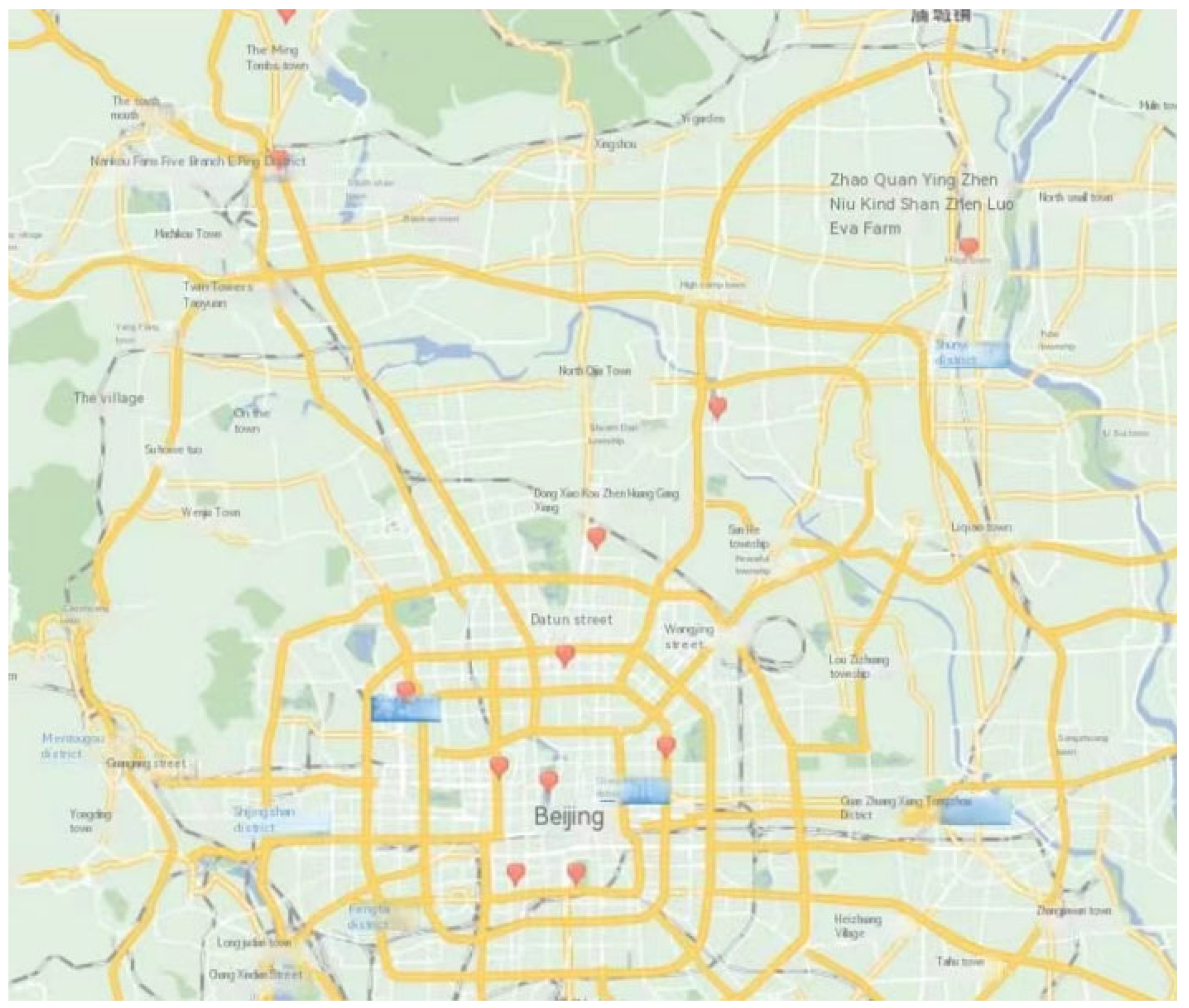
The experimental dataset utilized in this study was obtained from the environmental cloud of Nanjing Yunchuang Big Data Technology Co., LTD. (Nanjing, China) We accessed hourly meteorological records (comprising weather condition, air temperature, felt temperature, air pressure, humidity, rainfall, wind direction, and wind speed) and hourly air quality monitoring data (PM10, CO, SO2, NOx, O3) for Beijing, spanning from 1 January 2016 to 31 December 2016. The air quality monitoring data refer to the hourly data from 12 monitoring locations, resulting in a total of 8784 records for each monitoring point, though some data are missing due to uncontrollable factors. Missing data are mainly missing meteorological data, including missing meteorological data on a certain day and hour or missing wind direction data on a certain day and hour. If the entire meteorological data of a certain hour on a certain day are missing, the data are deleted. If the wind direction data of a certain hour on a certain day are missing, the linear interpolation method is used to complete the data. Thus, the final number of data records used was 8120. The locations of the 12 monitoring points are shown in Figure 1. Text descriptions of weather conditions, wind direction, and wind speed were encoded, as outlined in Table 1, Table 2 and Table 3.
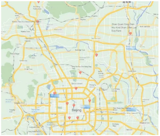
Figure 1.
Locations of 12 air quality monitoring points in Beijing in 2016.

Table 1.
Weather condition attribute coding rules in meteorological data.
Table 2.
Wind attribute coding rules in meteorological data.
Table 3.
Wind power attribute coding rules in meteorological data.
In the endeavor to construct and assess the predictive model, the dataset for each of the 12 monitoring points was partitioned into three categories: a predictive training set, predictive validation set, and a test set. The training set, which is integral to the three modules, comprises records 1 to 7000 from the dataset. The validation set is composed of data records 7001 to 7200, and the test set consists of records 7201 to 8120. Equipped with an Intel(R) Core(TM) i7-8565U CPU (Intel, Santa Clara, CA, USA) at 1.80 GHz, 8 GB of memory, and Windows 10 operating system, we used Python 3.7.8 (Guido van Rossum, Holland) as our programming tool for this experimental setup.
2.2. Framing
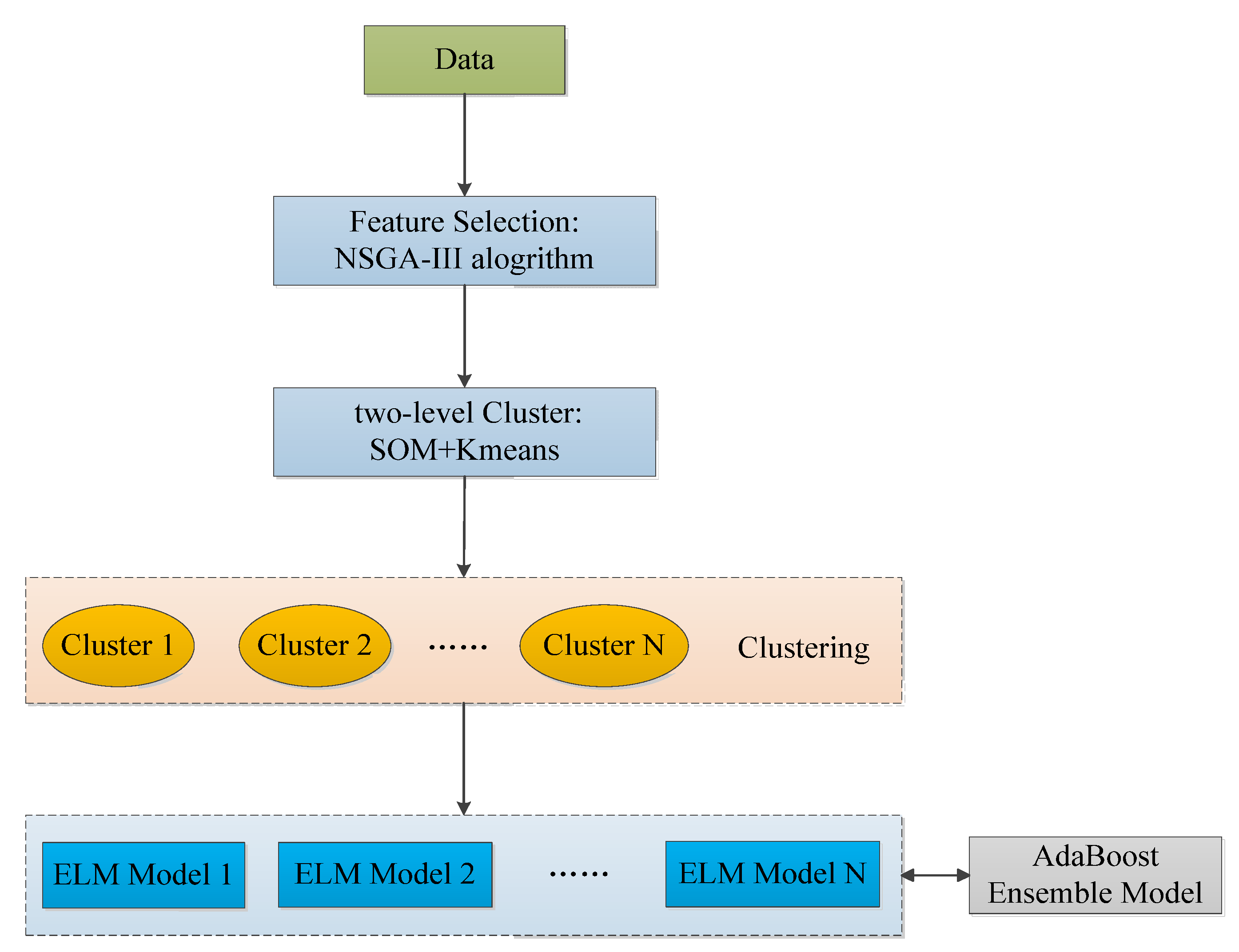
The conceptualized prediction model for PM2.5 concentration, dubbed as NSGA-III-SOM-Kmeans-Elm-Adaboost (NSKEA), is an integrated apparatus that primarily consists of three modules. Its main components are as follows:
- The utilization of NSGA-III for feature selection;
- Implementation of a two-layer clustering method (SOM-Kmeans) to cluster data post feature selection;
- Use the ELM model for the clustered data resulting from each cluster;
- Lastly, integration with AdaBoost is facilitated to realize the prediction of the PM2.5 concentration.
The inner structure of the proposed NSKEA model is conveniently illustrated in Figure 2. Therefore, a detailed investigation aids in understanding the intricate operations of this model.

Figure 2.
The structure of NSKEA algorithm.
2.3. Feature Selection: Multi-Objective Optimization: NSGA-III Algorithm
This study employs meteorological factors (such as air temperature, apparent temperature, air pressure, humidity, rainfall, wind direction, and wind speed) along with other air pollutants (PM10, CO, SO2, NOx, O3) as characteristic data in the feature selection process. It was found that these selected features had a strong correlation with PM2.5.
The aim of feature selection is identifying the optimal feature subset. It enables the elimination of irrelevant or redundant features, thus reducing the count of features, bettering the model’s precision, and decreasing the execution time.
Feature selection methodologies can be categorized into filtering method, wrapping method, and embedding method. Out of these, the wrapping method’s basic approach involves training the model for each feature subset to be selected on the training set. The feature subset is then chosen on the test set, based on the error magnitude.
In our feature selection module, we have taken the approach of the wrapping method, applying the NSGA-III algorithm for multi-objective optimization (MAE, MSE, and SD). It is used to compute the correlation between the predicted results of PM2.5 concentration for each feature and its actual value. Feature selection is performed by setting a specific threshold value.
The NSGA-III algorithm was first introduced by Kalyanmoy Deb and Himanshu Jain in 2014. This algorithm is an enhanced version of the multi-objective algorithm NSGA-II. It abandons the crowding-distance sorting mechanism often used in NSGA-II and introduces a new sorting mechanism based on reference points [26]. The NSGA-III is especially designed to deal with multi-objective optimization issues that have three or more objectives [27]. When compared with the NSGA-II algorithm, the NSGA-III not only significantly reduces the computational complexity but also excels in preserving diversity. This makes it an efficient tool for complex multi-objective optimization tasks.
The basic idea of using the NSGA-III algorithm for feature selection is as follows:
- The primary variables include PM10, CO, SO2, NOx, O3, air temperature, sensible temperature, air pressure, humidity, rainfall, wind direction, wind power, and wind speed, totaling 13 factors
- The focus for prediction is the PM2.5 concentration, identified as our target feature
- The Extreme Learning Machine (ELM) model is used individually with each feature as an input for prediction. Each feature’s predictive capability is assessed and an aggregated prediction is achieved using weighted reconstruction (Equation (1)),
- The evaluation is objective using the NSGA-III algorithm, taking into account the mean square error (MSE), Mean Absolute Error (MAE), and standard deviation (SD). These metrics, outlined in Equation (2) through (4), are deployed to measure the divergence between the predicted results and the actual values accurately,
- To realize multi-objective optimization featuring Mean Absolute Error (MAE), Mean Square Error (MSE), and Standard Deviation (SD), we harness the capabilities of the NSGA-III algorithm. Our strategy embodies an iterative search for a weight-set that concurrently minimizes MAE, MSE, and SD. Given the defined threshold value—, only those features that comply with the condition are selected. This precision-guided approach enables us to optimize feature selection effectively.
2.4. Two-Layer Clustering
Emphasizing the identification of anomalies in multifaceted datasets, we employ clustering algorithms, each providing a unique set of characteristics for the resulting clusters. Herein, we report the use of a two-layer clustering method employing a combination of Self-Organizing Maps (SOM) and K-means algorithms.
Initially, the SOM algorithm is applied to learn the data from the input space, which comprises 12 monitoring points; this serves to excavate similarities among them. Following acquisition of the prototype vector via this initial stage, the K-means algorithm is employed to cluster this vector, further extracting features of the training dataset. Our two-layer clustering methodology not only brings high-dimensional data visualization to fruition but also upholds the topological structure of input space while reducing dataset noise.
SOM, also known as Kohonen maps, are effectively used to visualize and explore data properties, projecting the input space onto a low-dimensional, regular grid prototype. This form of unsupervised learning is utilized to cluster data. Rooted in an uncomplicated concept, this type of neural network, with solely the input and competition layer, uses a “competitive learning” method during training. Each input sample seeks the most compatible node within the competitive layer, referred to as its activation node or “winning neuron” [28]. The parameters of this active node are updated via random gradient descent, while those of the nodes located near to the active node are suitably updated based on their proximity to it.
2.5. Prediction Model
To predict PM2.5 concentration levels, we have established a third module: a predictive model enhanced through ensemble learning methods. Unpackaging the outcomes from the two initial modules, we generate multiple cluster-resultant datasets, each accompanied by its respective ELM predictive model (Equation (5)).
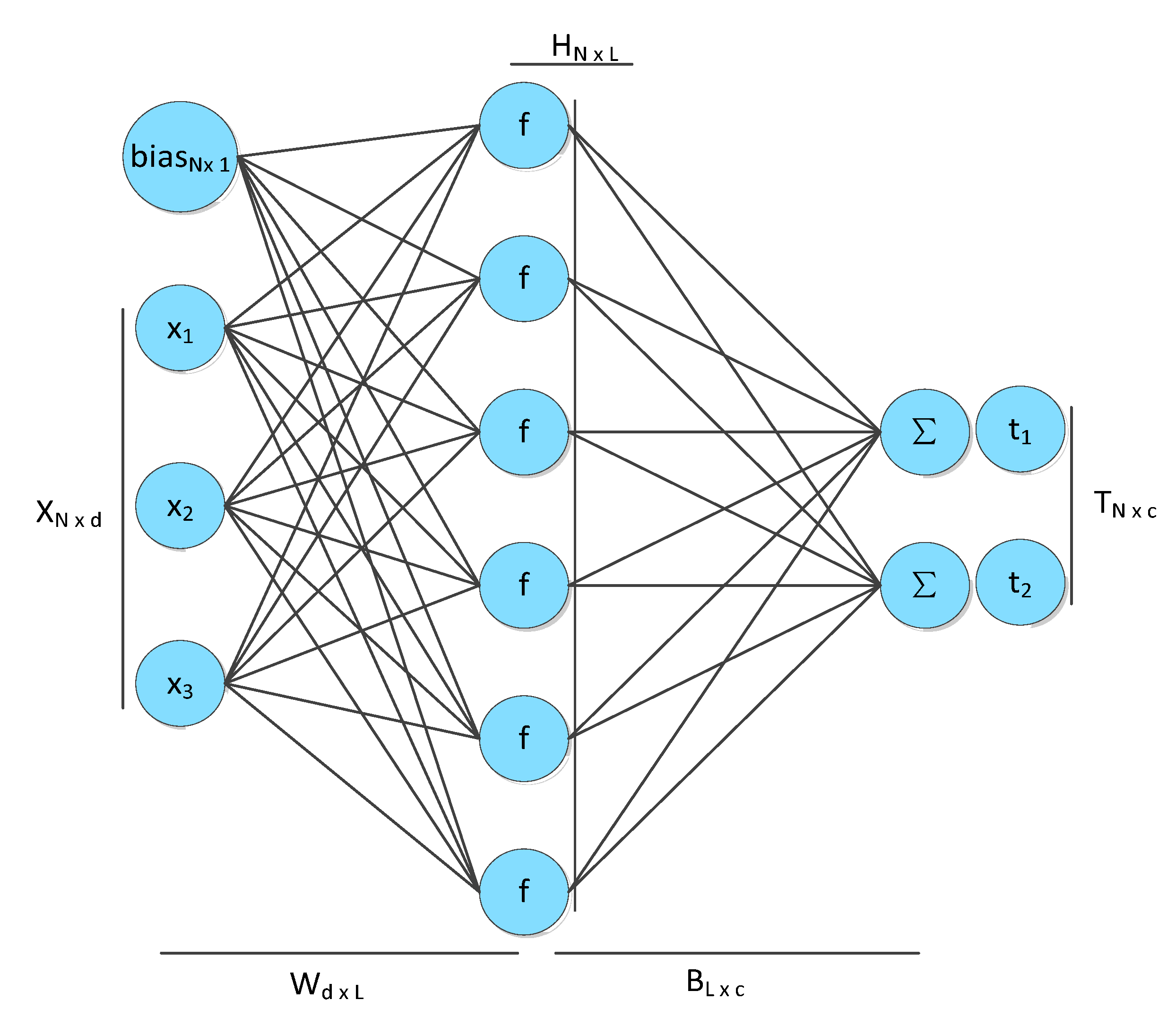
In this context, “” symbolizes the quantity of hidden units, while “” represents the count of training samples. “” designates the th weight vector interlinking the primary hidden layer and the output layer. The th input vector is represented by “”. “” stands for the weight vector connecting the th input layer to the output layer. The activation function is represented by “”. “” signifies a bias vector.
An ELM, a single-hidden-layer feedforward neural network (SLFN), is employed to expedite the training process [29]. This training methodology is notably superior to traditional SLFN algorithms, with ELM selecting random weights for input layers, hidden-layer bias, and output-layer weight, determined through minimization of a loss function—a sum of the training error term and a regular term reflecting the output-layer weight norm [30].
Despite the randomized generation of hidden-layer nodes, ELM preserves the fundamental approximation capacity of the SLFN. This network structure is depicted in Figure 3. ELM provides a rapid learning speed, robust generalization ability, and reduced parameter training dependency. Nonetheless, ELM disadvantages prevail; its exclusive focus on empirical risk inspires an overfitting proclivity remedied by introducing ensemble learning in this study.
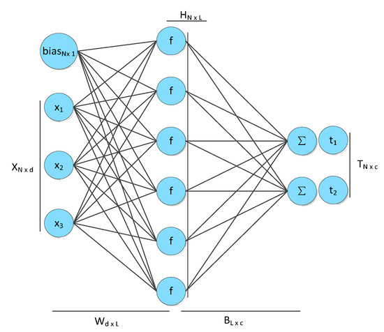
Figure 3.
Network structure of ELM.
Introduced by Yoav Freund and Robert Schapire in 1997, the Adaptive Boosting (AdaBoost) algorithm emerged as an innovative variant of the ensemble learning method, Boosting [31]. The adaptive nature of this algorithm comes to the fore in its weighting strategy; training errors result in increased sample weights, whereas correctly classified samples see a decrease, readying them for training in succeeding basic classifiers. Moreover, with each iterative cycle, a new weak classifier is incorporated into the ensemble until either achieves a predefined minimum error rate or reaches the maximum number of iterations.
The procedure for an AdaBoost ensemble prediction model utilizing an Extreme Learning Machine (ELM) as a base classifier unfolds as follows:
Step 1: Initiate the weight distribution for each ELM base classifier such that each classifier assumes an equal weight of . This process generates the initial weight distribution, denoted as , across the training sample set. The setup is defined by Equation (6).
Step 2: Iterative Process:
- (a)
- From the collection of weak classifiers, identify the classifier with the lowest current error rate. This is designated as the -base classifier, , and calculate its value . The corresponding error and distribution of the weak classifier are enumerated in Equation (7).
- (b)
- Ascertain the weight of the weak classifier within the final classifier ensemble (Equation (8)).
- (c)
- Update the weight distribution (Equation (9)) for the training sample set.
Here, it is essential to note that represents the normalization constant .
Step 3: Compile each weak classifier ELM according to its weight. In the final stage, this integration generates the robust final classifier, (Equations (10) and (11)), which then delivers the predictive output.
3. Case Study
3.1. Evaluation Criteria
To assess the efficacy of the prediction model, we conduct an inclusive evaluation using a threefold metric of MAE, Root Mean Square Error (RMSE), and the index of agreement (IA, a nondimensional and bounded measure of the model prediction error degree with values closer to 1 indicating a better match). The calculated formulae for these parameters can be found in Table 4. Within these formulae, the variables and signify the predicted and observed PM2.5 concentrations, respectively, the variable is the average value of observed PM2.5 concentrations, whereas stands for the total number of predicted values.
Table 4.
Evaluation criteria.
3.2. Experimental Design
3.2.1. The NSGA-III Based Feature Selection Method Analysis
To validate the feasibility and precision of the feature selection method proposed herein, we designed three prediction models for comparative analysis—the NSGA-III-ELM-Adaboost (NEA) model; the single factor-ELM-AdaBoost (SFEA), a unifactorial ensemble model centered solely on PM2.5 concentration features; and the all features-ELM-Adaboost (AFEA) model, an ensemble model incorporating all features. For consistency and to ensure the legitimacy of our comparative results, all three models employ an ELM-Adaboost model and keep the integrated model parameters consistent.
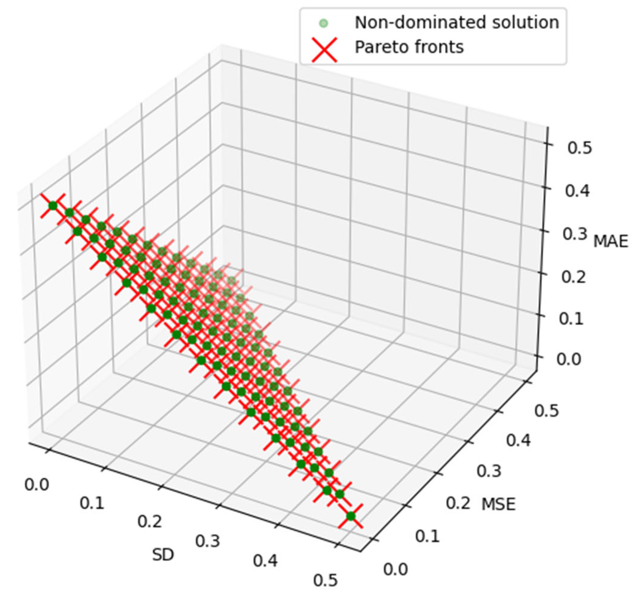
The NEA model’s parameter settings can be found in Table 5. Figure 4 depicts the results of the Pareto fronts and the selected point from the one-step predicted dataset. We chose the intermediate solution of Pareto fronts to harmonize the benefits from the three objective functions. Figure 5 represents the optimal weight results for each feature in a 12-point monitoring dataset. Table 6 presents a comparative analysis of the evaluation indicators from the three prediction models.
Table 5.
Parameter setting of the NSGA-III-ELM-Adaboost model.

Figure 4.
Pareto fronts and the selected solutions of dataset.
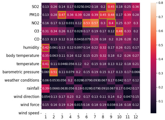
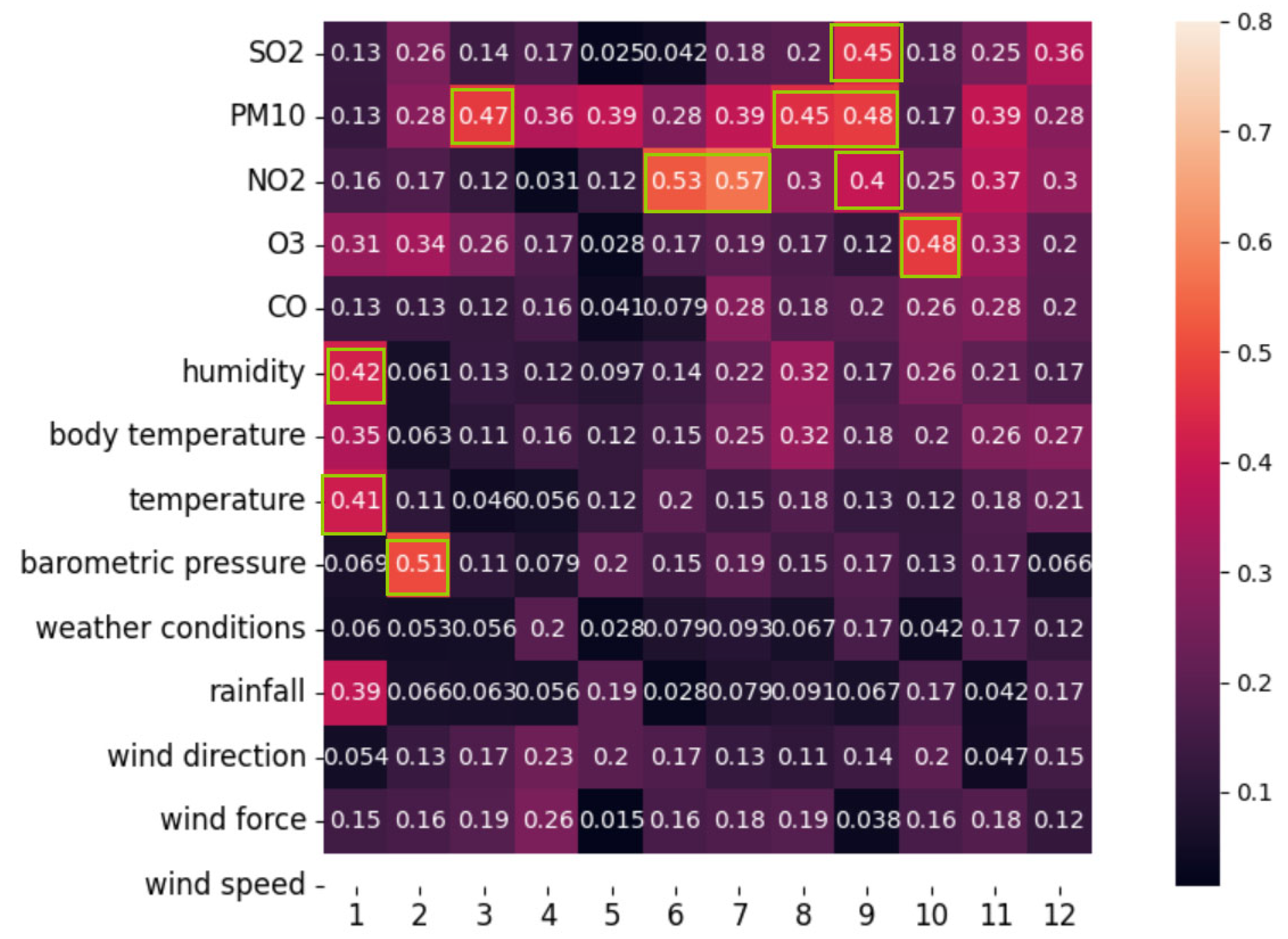
Figure 5.
Optimal weight results for each feature of a dataset of 12 monitoring points.
Table 6.
Comparison of evaluation criteria of six prediction models.
Employing the tenfold cross-validation method, the threshold for the NSGA-III feature selection stage was determined as . Each feature’s weight was compared with this threshold, and those with a weight () equal to or surpassing 0.4 were selected, as exemplified by the results of the 12-point monitoring study (Figure 4). Consequently, seven features—namely SO2, PM10, NO2, O3, humidity, temperature, and barometric pressure—were chosen as the input data for the prediction model.
The experimental evaluations from three distinct models, presented in Table 6, underscore that the NEA predictions at 12 monitoring points are most favorable after feature selection via NSGA-III. This finding substantiates that a feature selection strategy premised on the NSGA-III algorithm can indeed enhance the accuracy of the prediction model.
3.2.2. Ensemble Model Analysis
In this section, we analyze the experimental outcomes of a two-layer clustering method (SOM+Kmeans). As delineated in Section 3.2, the SOM algorithm is initially employed for cluster learning on datasets subject to feature selection, contingent on NSGA-III. This is subsequently followed by using the K-means algorithm to cluster the prototype vector, thus further mining the features of the training dataset.
To critically assess the number of clusters, we utilize evaluation metrics such as F-measure, Accuracy, and Normalized Mutual Information. These indicators range between [0, 1], where a larger value signifies that the clustering outcome is commensurate with expectations.
Table 7 encapsulates the calculation formulas of these three metrics. True Positive (TP) denotes the positive predicted sample count, while True Negative (TN) indicates the negative predicted count. False Positive (FP) represents instances where the predicted class number is wrongly marked as positive, whereas False Negative (FN) refers to samples falsely predicted as negative. Entropy of correct classification is represented as H(U), and H(V) stands for the entropy of results obtained via the algorithm.
Table 7.
Evaluation index of clustering results.
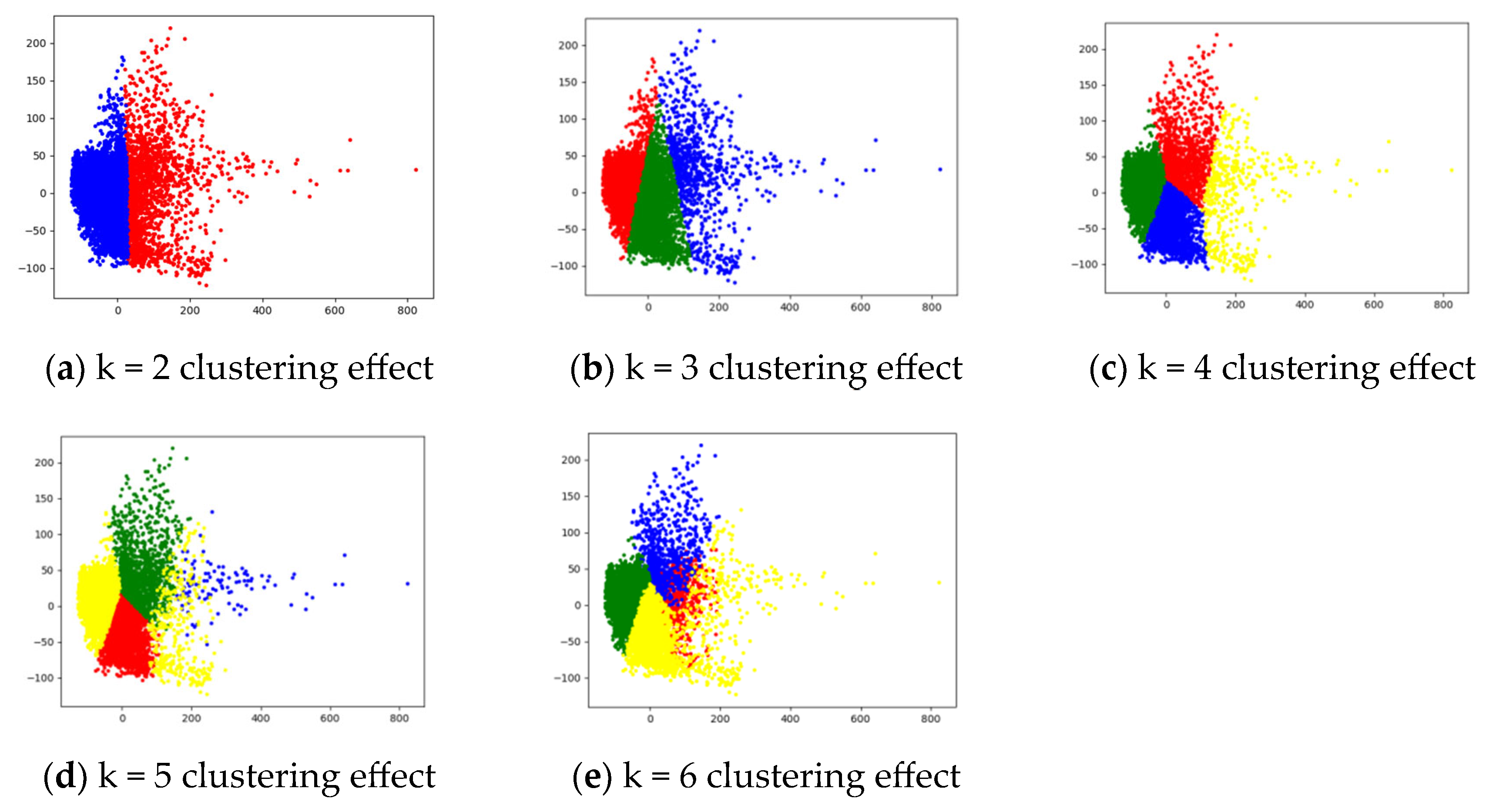
Data collated from three evaluation indicators, for differing cumulative cluster numbers, are presented in Table 8. Figure 6, meanwhile, portrays the variance in clustering efficacy in relation to fluctuating cluster numbers. An impartial analysis of both Table 8 and Figure 5 highlights that the number of clusters yielding the most optimal result across all three indices, and the most conducive clustering effect, when .
Table 8.
Results of three evaluation indexes with different number of clusters.

Figure 6.
Clustering effect under different number of clusters.
3.3. Discussion
In this section, in order to prove the predictive superiority of our forecasting method, five existing air pollution forecasting models (RNN, LSTM, MLR, SVR, and RF) and three models given in 4.2.1 (NEA, SFEA, and AFEA) are compared with the proposed model. All models were tested using the data in Section 2.1, and the average error index data were obtained, as shown in Table 6.
In all comparative experiments, the evaluation index results, as measured by NSKEA at every monitoring point, are identical. Specifically, during the second phase, data from the twelve monitoring points are aggregated, amplifying similarities among these points, to yield a single, unique final prediction result. As can be seen from Table 6, in the experimental dataset, the error evaluation index data of NSKEA algorithm are the smallest, while IA index data are the largest, and the values of MAE, RMSE and IA are 13.418 µg/m3, 21.401 µg/m3 and 0.93, respectively. It shows that the prediction effect of NSKEA algorithm is the best.
By comparing the index data of the NEA, SFEA, and AFEA models in Table 6, it is found that the three indicator data of NEA are the best. This suggests that feature selection within the original dataset positively influences the model’s predictive accuracy, further hinting at a nonlinear relationship existing between the attributes. This highlights the need for machine learning methods to probe deeper into these mutual feature relationships.
When comparing NSKEA, RNN, and LSTM, NSKEA emerged supreme. This suggests that contrasted with standalone models, a comprehensive learning model that dynamically selects the dataset’s beneficial features and adjusts the weak prediction model’s weight ratios using the proposed prediction mechanism, is more efficient. By being adaptable, the predictive model can deliver more accurate PM2.5 concentration forecasts.
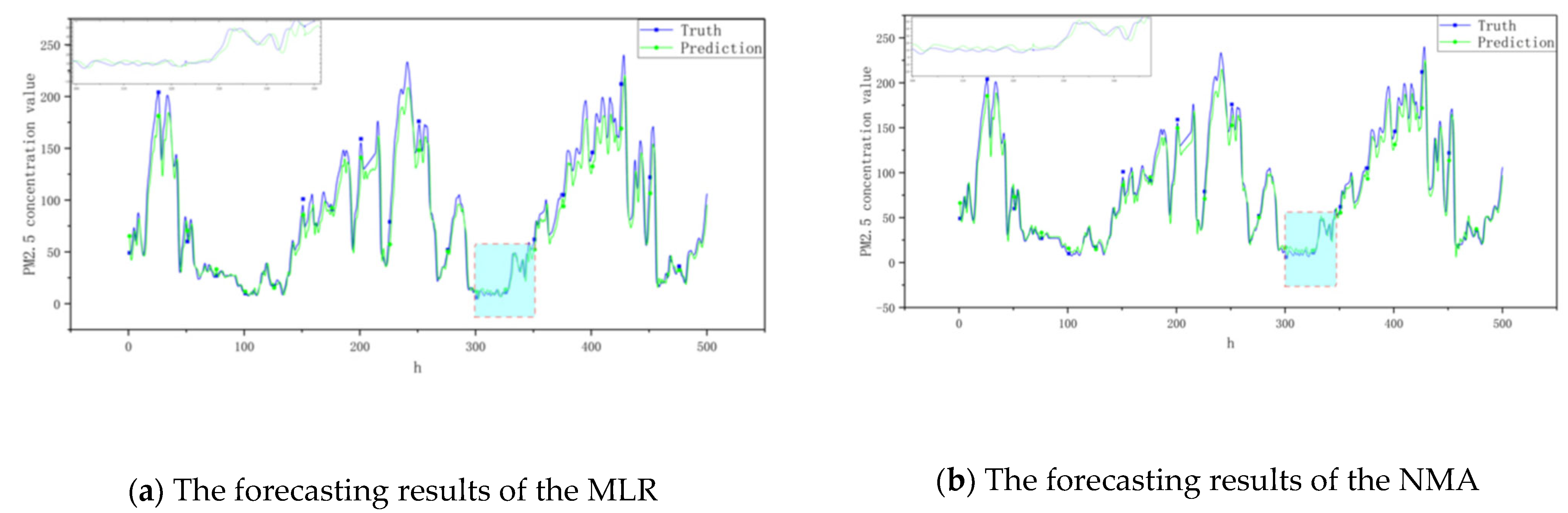
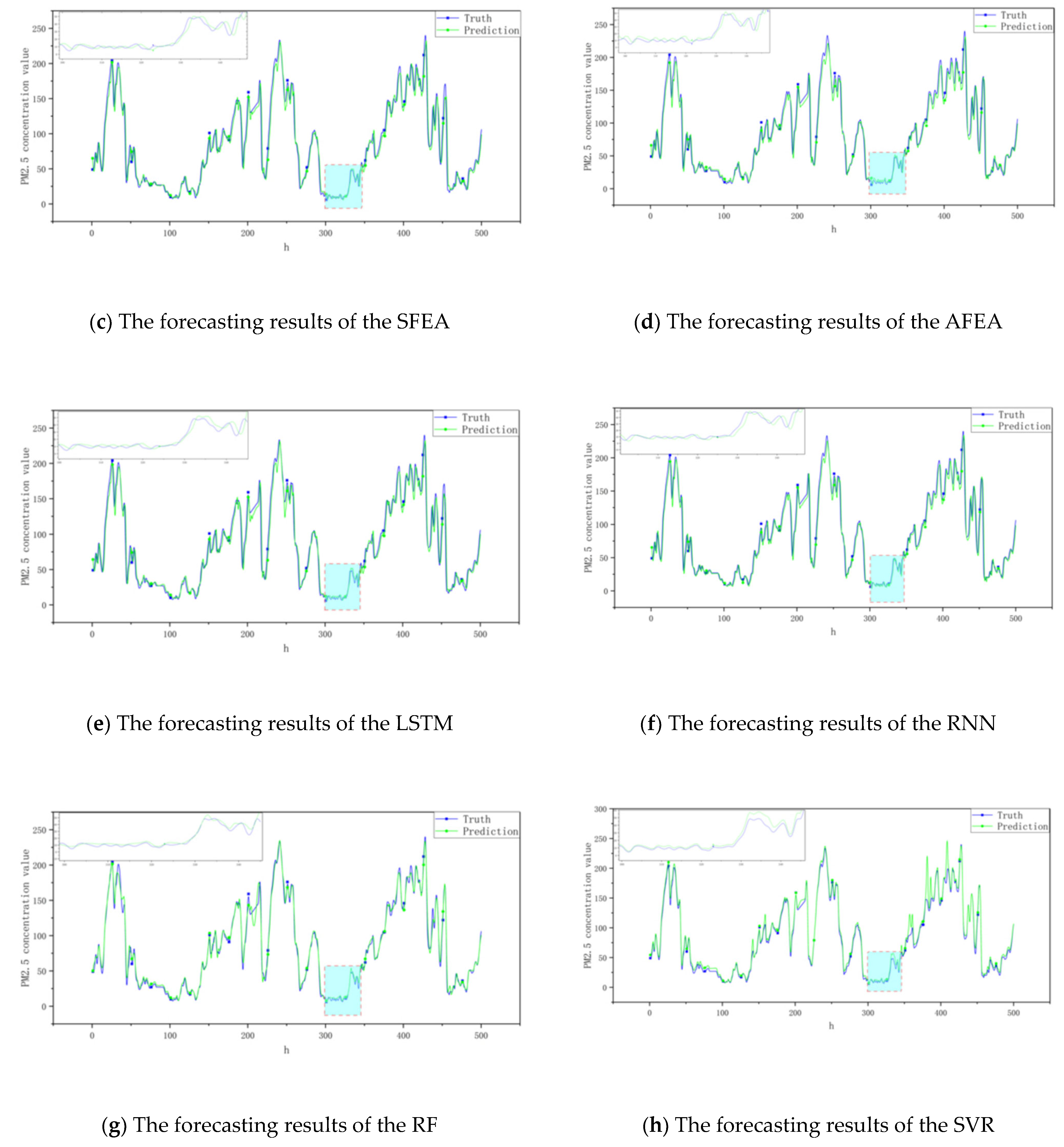
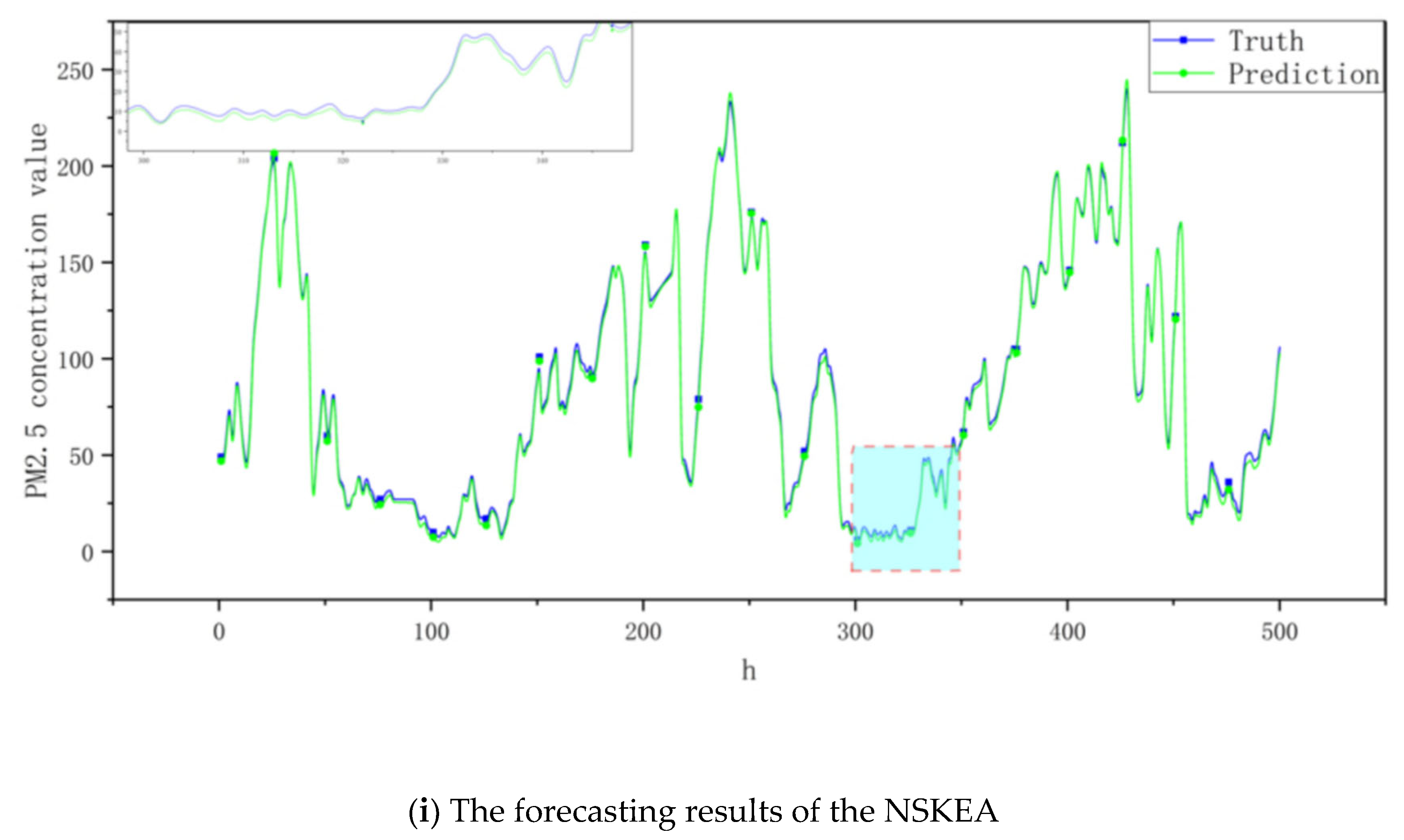
Because of the space limitation of the paper, we only give the prediction results of nine models on the first observation point dataset, as shown in Figure 7. By comparing the observed values and prediction results of each model on the dataset, it can be seen that the prediction results of the NSKEA model are the most consistent with the observed values, and the accuracy rate is 95.6%. Accordingly, the proposed model significantly enhances the overall prediction performance.
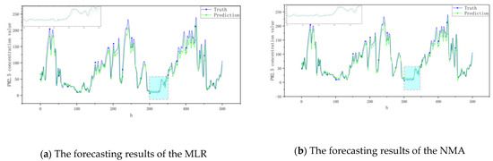
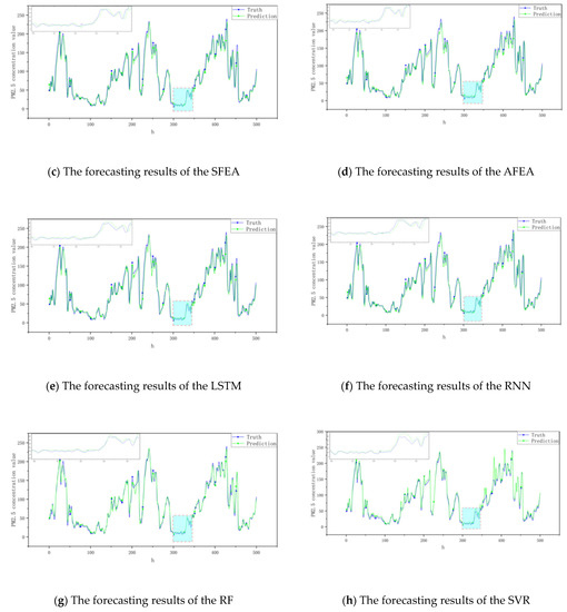
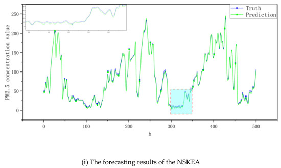
Figure 7.
The prediction results of nine models at the first observation point.
4. Conclusions
Rapid global climate change has led to escalating concerns surrounding air pollution, with adverse effects increasingly infringing upon daily life. As awareness of environmental conditions grows, so too does the demand for improved air quality. This increased societal pressure makes the urgent task of meticulous pollution prevention and control management necessary. Simultaneously, while sustaining rapid economic development, minimizing industrialization’s environmental and climatic impact has emerged as a shared objective sought by global academicians. Therefore, the scientific, accurate monitoring of air quality and pollutant concentrations, alongside understanding the pollution variation laws and environmental impacts of air pollution severity, offers strategic advantages. This knowledge promotes precisely guided pollution control measures and is critical for fostering healthy urban development.
This manuscript introduces a multifactorial model predicting PM2.5 concentration levels within the atmosphere. The described method integrates feature selection, clustering, and ensemble learning techniques to deep-mine original dataset in-house features, thereby augmenting the model’s predictive precision. Key findings from the experimental outcomes highlight:
- (1)
- The model outlined herein enhances PM2.5 concentration prediction accuracy. Demonstrating significant adaptability, the NSKEA model capably mines data, evident in its performance amidst PM2.5 seasonal fluctuations.
- (2)
- Implementing multi-objective optimization for multi-factor feature selection supports enhanced diversity preservation, consequential in advancing the predictive model’s precision.
- (3)
- The study employed the ELM as a weak learner without considering variations in the prediction model in light of diverse basic learners. Future research will explore this area further, focusing on identifying the optimal basic learner to enhance the robustness and accuracy of the integrated predictive model.
Author Contributions
Conceptualization, X.W.; methodology, X.W.; software, X.W. and Q.W.; validation, X.W. and J.Z.; formal analysis, X.W. and Q.W.; resources, X.W. and Q.W.; data curation, X.W. and J.Z.; writing—original draft preparation, X.W.; writing—review and editing, X.W.; project administration, Q.W.; funding acquisition, Q.W. and J.Z. All authors have read and agreed to the published version of the manuscript.
Funding
This research was funded by [the Project of Outstanding Talents in Universities of Anhui Province] grant number [GXYQ2022075], and [the Project of Key Laboratory of Anhui Province] grant number [IBES2021KF07].
Institutional Review Board Statement
Not applicable.
Informed Consent Statement
Not applicable.
Data Availability Statement
Not applicable.
Conflicts of Interest
The authors declare no conflict of interest.
References
- Jamei, M.; Ali, M.; Malik, A.; Karbasi, M.; Sharma, E.; Yaseen, Z.M. Air quality monitoring based on chemical and meteorological drivers: Application of a novel data filteringbased hybridized deep learning model. J. Clean. Prod. 2022, 374, 134011. [Google Scholar] [CrossRef]
- Niu, M.; Wang, Y.; Sun, S.; Li, Y. A novel hybrid decomposition-and-ensemble model based on CEEMD and GWO for short term PM2.5 concentration forecasting. Atmos. Environ. 2016, 134, 168–180. [Google Scholar] [CrossRef]
- Yin, S.; Liu, H.; Duan, Z. Hourly PM2.5 concentration multi-step forecasting method based on extreme learning machine, boosting algorithm and error correction model. Digit. Signal Process. 2021, 118, 103221. [Google Scholar] [CrossRef]
- Ren, C.R.; Xie, G. Prediction of PM2.5 concentration level based on random forest and meteorological parameters. Comput. Eng. Appl. 2019, 55, 213–220. [Google Scholar]
- Hong, K.Y.; Pinheiro, P.O.; Weichenthal, S. Predicting global variations in outdoor PM2.5 concentrations using satellite images and deep convolutional neural networks. arXiv 2019, arXiv:1906.03975v1. [Google Scholar]
- Wu, X.X.; Zhang, C.; Zhu, J.; Zhang, X. Research on PM2.5 concentration prediction based on the CE-AGA-LSTM model. Appl. Sci. 2022, 12, 7009. [Google Scholar] [CrossRef]
- Pruthi, D.; Liu, Y. Low-cost nature-inspired deep learning system for PM2.5 forecast over Delhi, India. Environ. Int. 2022, 166, 107373. [Google Scholar] [CrossRef]
- Zaini, N.; Ean, L.W.; Ahmed, A.N.; Malek, M.A.; Chow, M.F. PM2.5 forecasting for an urban area based on deep learning and decomposition method. Sci. Rep. 2022, 12, 17565. [Google Scholar] [CrossRef]
- Li, W.L.; Jiang, X.C. Prediction of air pollutant concentrations based on TCN-BiLSTM-DMAttention with STL decomposition. Sci. Rep. 2023, 13, 4665. [Google Scholar] [CrossRef]
- Zhou, Y.L.; Chang, F.J.; Chang, L.C.; Kao, I.F.; Wang, Y.S. Explore a deep learning multi-output neural network for regional multi-step-ahead air quality forecasts. J. Clean. Prod. 2019, 209, 134–145. [Google Scholar] [CrossRef]
- Hu, S.; Liu, P.F.; Qiao, Y.X.; Wang, Q.; Zhang, Y.; Yang, Y. PM2.5 concentration prediction based on WD-SA-LSTM-BP model: A case study of Nanjing city. Environ. Sci. Pollut. Res. 2022, 29, 70323–70339. [Google Scholar] [CrossRef] [PubMed]
- Huang, J.; Zhang, F.; Du, Z.H.; Liu, R.Y.; Cao, X.P. Hourly concentration prediction of PM2.5 based on RNN-CNN ensemble deep learning model. J. Zhejiang Univ. (Sci. Ed.) 2019, 46, 370–379. [Google Scholar]
- Liu, X.L.; Tan, W.A.; Tang, S. A Bagging-GBDT ensemble learning model for city air pollutant concentration prediction. In Proceedings of the IOP Conference Series: Earth and Environmental Science, Gothenburg, Sweden, 8–12 October 2019. [Google Scholar]
- Liu, H.; Yang, R. A spatial multi-resolution multi-objective data-driven ensemble model for multi-step air quality index forecasting based on real-time decomposition. Comput. Ind. 2021, 125, 103387. [Google Scholar] [CrossRef]
- Liu, B.; Tan, X.H.; Jin, Y.Q.; Yu, W.W.; Li, C.Y. Application of RR-XGBoost combined model in data calibration of micro air quality detector. Sci. Rep. 2021, 11, 15662. [Google Scholar] [CrossRef] [PubMed]
- Joharestani, M.; Cao, C.X.; Ni, X.L.; Bashir, B.; Joharestani, S. PM2.5 Prediction Based on Random Forest, XGBoost, and Deep Learning Using Multisource Remote Sensing Data. Atmosphere 2019, 10, 373. [Google Scholar] [CrossRef]
- Wei, L.X.; Zhang, L.Y.; Wang, H. Impact analysis and simulation study of air pollution and meteorological conditions in Baoding city. Environ. Dev. 2018, 30, 162–163. [Google Scholar]
- Liu, T.; Wu, M.P.; Zhang, K.D.; Liu, Y.; Zhong, J. Correlation Analysis and Control Scheme Research on PM2.5. Appl. Mech. Mater. 2014, 590, 888–894. [Google Scholar] [CrossRef]
- Zeng, J.; Wang, M.E.; Zhang, H.X. Correlation between atmospheric PM2.5 concentration and meteorological factors during summer and autumn in Beijing, China. J. Appl. Ecol. 2014, 25, 2695–2699. [Google Scholar]
- Wei, Y.Y.; Chen, Z.Z.; Zhao, C.; Chen, X.; He, J.H.; Zhang, C.Y. A time-varying ensemble model for ship motion prediction based on feature selection and clustering methods. Ocean Eng. 2023, 270, 113659. [Google Scholar] [CrossRef]
- Redkar, S.; Mondal, S.; Joseph, A.; Hareesha, K.S. A machine learning approach for drug-target interaction prediction using wrapper feature selection and class balancing. Mol. Inform. 2020, 39, 1900062. [Google Scholar] [CrossRef]
- Wu, H.P.; Liu, H.; Duan, Z. PM2.5 concentrations forecasting using a new multi-objective feature selection and ensemble framework. Atmos. Pollut. Res. 2020, 11, 1187–1198. [Google Scholar] [CrossRef]
- Got, A.; Moussaoui, A.; Zouache, D. Hybrid filter-wrapper feature selection using whale optimization algorithm: A multi-objective approach. Expert Syst. Appl. 2021, 183, 115312. [Google Scholar] [CrossRef]
- Han, F.; Chen, W.T.; Ling, Q.H.; Han, H. Multi-objective particle swarm optimization with adaptive strategies for feature selection. Swarm Evol. Comput. 2021, 62, 100847. [Google Scholar] [CrossRef]
- Vesanto, J.; Alhoniemi, E. Clustering of the self-organizing map. IEEE Trans. Neural Netw. 2000, 11, 586–600. [Google Scholar] [CrossRef] [PubMed]
- Deb, K.; Jain, H. An evolutionary many-objective optimization algorithm using reference point-based nondominated sorting approach, Part I: Solving problems with box constraints. IEEE Trans. Evol. Comput. 2014, 18, 577–601. [Google Scholar] [CrossRef]
- Fei, P.; Li, Z.; Zhu, D.; Yu, X. Multi-objective multi-learner robot trajectory prediction method for IoT mobile robot systems. Electronics 2022, 11, 2094. [Google Scholar]
- Wang, Y.K.; Chen, X.B. A joint optimization QSAR model of fathead minnow acute toxicity based on a radial basis function neural network and its consensus modeling. RSC Adv. 2020, 10, 21292–21308. [Google Scholar] [CrossRef] [PubMed]
- Wei, Y.Y.; Chen, Z.Z.; Zhao, C.; Chen, X.; He, J.H.; Zhang, C.Y. A threestage multi-objective heterogeneous integrated model with decompositionreconstruction mechanism and adaptive segmentation error correction method for ship motion multi-step prediction. Adv. Eng. Inform. 2023, 56, 101954. [Google Scholar] [CrossRef]
- Yang, X.T.; Bao, Z.X.; Wang, G.Q.; Liu, C.S.; Jin, J.L. Trends and changes in hydrologic cycle in the Huanghuaihai river basin from 1956 to 2018. Water 2022, 14, 2148. [Google Scholar] [CrossRef]
- Freund, Y.; Schapire, R.E. A decision-theoretic generalization of on-line learning and an application to boosting. J. Comput. Syst. Sci. 1997, 55, 119–139. [Google Scholar] [CrossRef]
Disclaimer/Publisher’s Note: The statements, opinions and data contained in all publications are solely those of the individual author(s) and contributor(s) and not of MDPI and/or the editor(s). MDPI and/or the editor(s) disclaim responsibility for any injury to people or property resulting from any ideas, methods, instructions or products referred to in the content. |
© 2023 by the authors. Licensee MDPI, Basel, Switzerland. This article is an open access article distributed under the terms and conditions of the Creative Commons Attribution (CC BY) license (https://creativecommons.org/licenses/by/4.0/).