Article

Study on Spatial and Temporal Distribution Characteristics of the Cooking Oil Fume Particulate and Carbon Dioxide Based on CFD and Experimental Analyses

1
Faculty of Maritime and Transportation, Ningbo University, Ningbo 315000, China
2
Fotile Group Ningbo Fotile Kitchenware Co., Ltd., Ningbo 315336, China
3
Healthy & Intelligent Kitchen Engineering Research Center of Zhejiang Province, Ningbo 315204, China
*
Author to whom correspondence should be addressed.
Atmosphere 2023, 14(10), 1522; https://doi.org/10.3390/atmos14101522
Submission received: 14 July 2023 / Revised: 1 August 2023 / Accepted: 2 August 2023 / Published: 30 September 2023
(This article belongs to the Special Issue Health and Environmental Effects of Particulate Matter)

Abstract

:
The cooking oil fume particulate (COFP) produced by indoor cooking can harm human health seriously, and therefore requires urgent monitoring and optimization. In this paper, the kitchen cooking simulation process was established by using computational fluid dynamics (CFD) based on the fluid dynamics theory. Combined with the user defined function (UDF), the spatial and temporal distributions of COFP and carbon dioxide (CO2) during the cooking process were simulated and analyzed, respectively. Both simulation results were verified using experimental data. Moreover, this paper introduces a COFP concentration correlation function that utilizes the spatiotemporal correlation between COFP and CO2 concentrations during the cooking process. The function is based on the spatiotemporal distribution of CO2 concentration. By comparing it with traditional calculations, the proposed function is shown to achieve a remarkable 70% improvement in efficiency and maintain an accuracy rate exceeding 90%. This enables the rapid analysis and control of COFP concentration through monitoring and analyzing CO2 levels in the kitchen.

1. Introduction

With the speedy development of modern industry and the rapid progress of urbanization, air pollution has become an increasingly severe environmental problem [1,2]. Among them, particulate matter (PM) has been recognized for its harm to human health as one of the main pollutants [3]. Such particles may lead to respiratory diseases, cardiovascular diseases, and other health problems, causing significant economic and social burdens worldwide [4]. It was reported that humans spend about 70% to 90% of their total activity time indoors [5]. However, indoor environments can be seriously polluted by activities such as cooking in the kitchen and smoking. In the enclosed and small space of the kitchen, frequent high-temperature cooking processes can generate a large amount of cooking oil fume particulate (COFP), exacerbating indoor pollution [6]. Therefore, analyzing and controlling the temporal and spatial distribution characteristics of COFP in kitchen cooking environments has become an important research area for protecting human health and improving indoor air quality.
The movement, settling, and diffusion of fine particles in indoor environments are influenced by various factors, including heat sources, ventilation conditions, and fresh air systems [7]. To investigate the concentration distribution of indoor particulate matter, researchers have conducted various experimental tests. For example, Wang used environmental scanning electron microscopy (ESM) and other technologies to study the emission characteristics of ultrafine particles (UFP) during residential solid fuel combustion [8]. Xiang measured the UFP concentration during cooking processes in the kitchen, living room, and bedroom in different environments by using the P-Trak condensation nucleus counter [9]. In addition, Zhou further developed a new quantitative indoor particle matter prediction model based on the monitoring results of particle concentration changes in the hospital outpatient hall using the LD-6S multi-functional laser particle analyzer [10]. However, there are some difficulties in monitoring particulate matter such as the limited monitoring range, high experimental costs, etc. In recent years, with the development of computer technology, more and more numerical simulation studies have been used to simulate the transport, diffusion, and settling mechanisms of fine particles in indoor environments [11]. Currently, computational fluid dynamics (CFD) has become a widely used method in the study of indoor particle matter diffusion, as it can effectively reflect the motion and distribution of indoor particle matter [12]. The Lagrangian method or Eulerian method can be used for gas–particle two-phase coupling calculation [13]. The Lagrangian approach is a method of discretizing particles individually, and the motion trajectory of each particle is obtained by solving the Reynolds average Navier–Stokes (RANS) over the entire flow region. This method can also be referred to as the Lagrangian Discrete Random Walk (DRW) model [14]. The Eulerian method assumes that particles are a continuous medium and establishes a particle concentration transport equation based on the mass conservation equation. The method is also known as the Drift Flux (DF) model, which assumes the particles to be a continuous medium and establishes the particle concentration transport equation based on the mass conservation equation [15]. Recent studies have shown that the DRW model can predict the diffusion of indoor particle matter very well [16]. But its accuracy is lower in the places near the boundary and/or close to the wall. The DF model has been used to study the impact of particle dispersion in both indoor and outdoor environments, but its settlement rate is mostly based on the empirical value or sometimes even ignored. Currently, a sound framework for monitoring and predicting indoor particle matter emissions has not yet been established, partially due to the significant computational resources and time required for conducting gas–particle two-phase coupled numerical simulations. There are some challenges in developing such a framework and to implement corresponding computer simulations.
In summary, this paper focuses on an experimental kitchen and monitors the COFP and carbon dioxide (CO2) produced during indoor cooking processes. A numerical simulation process for COFP and CO2 was established by using CFD. The reliability of the simulation process was verified and confirmed by comparing the experimental results and simulation results. Furthermore, in view of the difficulty in monitoring COFP and the long computation time of computer simulations for COFP, this paper focuses on exploring the correlation between COFP and CO2 in the space near the human body. A relationship function between the concentrations of COFP and CO2 is established to reduce the cost of monitoring and analysis of COFP.

2. Experimental Testing

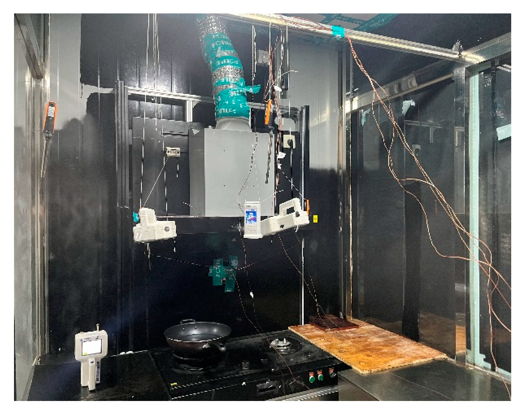
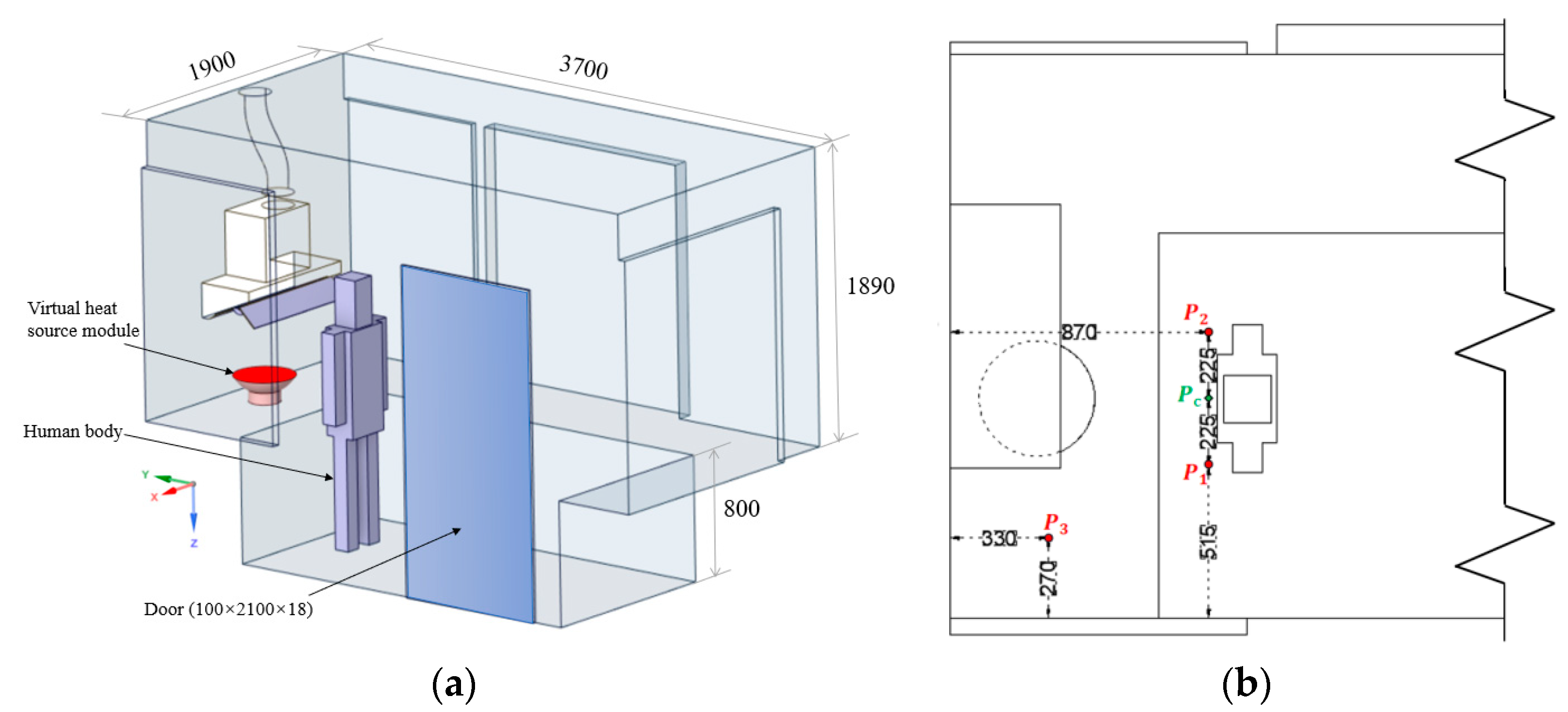
2.1. Experimental Kitchen Layout and Test Parameters

Figure 1 shows a fully enclosed transparent experimental kitchen with a stove height of 800 mm. The distance between the range hood and the stove is 750 mm. The dimensions of the doors are 2100 mm and 1000 mm for length and width, respectively, and all four door gaps are 18 mm in width. The diameter of the pot bottom is 390 mm, and the distance between the human body and the stove is 200 mm.
The Handheld3016 model is selected as the particle counter, which features six particle size standard channels (0.3, 0.5, 1.0, 3.0, 5.0, 10.0). It operates in pumping sampling mode with a flow rate of 0.1 ft3/min and it exhibits a typical accuracy of less than 10%. The ST8310A model is selected to record CO2 concentrations, which offers a measurement range of 0 to 3000 ppm with a resolution of 1 ppm. The Handheld3016 and the ST8310A were used to monitor the concentrations of COFP and CO2. Measurement points P 1 , P 2 , P 3 ,   a n d   P c are located at heights of 1600 mm, 1600 mm, 1060 mm, and 1650 mm above the ground, respectively. The specific locations are shown in Figure 2b. The test object of this experiment is fried potato strips. A total of seven tests were conducted, and the testing parameters are shown in Table 1. The air in the immediate vicinity of the human face has a direct impact on respiration and overall human health, making it a crucial local air zone. To ensure precise calculations for this important area, the COFP monitoring points P 1 and P 2 and the CO2 monitoring point P c are strategically placed within this local air region. The experimental data collected from these monitoring points serves as a direct benchmark for validating the accuracy of the calculations within this specific air zone. It is worth noting that the accuracy of the calculation for this vital local air domain is not indirectly inferred through the verification of other monitoring points. Additionally, the COFP monitoring point P 3 is positioned on the left panel to ensure the simulation calculations maintain accuracy within the broader calculation domain.
To establish a general rule of the experimental data, the paper carefully planned the process of heating, cooking, and cooling the shredded potatoes. The total time for this process was set at 3 min, equivalent to 270 s. To avoid the uncertainty of the experiment, the process was repeated 8 times. Additionally, to account for any potential experimental accidents, a fault tolerance time of 90 s was included before the start of the experiment. Hence, the total experimental duration was set as 2250 s.

2.2. Test Results and Analysis

Figure 3 depicts the experimental testing process, while Figure 4 displays the data of COFP at each monitoring point. Figure 3 shows the experimental testing flowchart, and Figure 4 presents the data for each monitoring point of COFP, where both COFP concentration and CO2 concentration exhibit significant fluctuations. Starting from the third period, the concentration variations at different monitoring points tend to follow a similar pattern. The COFP concentration values of monitoring points P 1 and P 2 are similar, located at the same height on both sides of the face. The peak value is reached after cooking for 90 s and is about 70 μ g / m 3 . The fluctuation range is greater than that of the concentration measured at the stove. The variation of COFP concentration at monitoring point P 3 on the stove is affected by the particle settling rate, resulting in a time lag in its peak concentration, which is approximately 40 μ g / m 3 . The CO2 concentration at monitoring point P c in front of the face shows a regular variation pattern with a bimodal phenomenon, and its peak value is approximately 920 ppm. The bimodal phenomenon is attributed to errors in the data acquisition process, which includes systematic and human errors. Systematic errors may arise from instrument inaccuracies, although these errors are typically small and have minimal impact on the overall results. On the other hand, human errors play a more significant role in this experiment. The first peak occurs within the 120 to 150 s timeframe during the cooking process and is primarily caused by the CO2 emissions generated from the cooking activity. This initial peak is expected and deserves particular attention during analysis. The second peak, observed between 180 and 240 s, is independent of the cooking process. It is predominantly influenced by human activities occurring after cooking, such as people moving around, which can disrupt air circulation and lead to a temporary increase in CO2 levels. Additionally, the human body itself emits carbon dioxide, as breathing releases a higher concentration of this gas.

3. Numerical Calculation

3.1. Numerical Method

The governing equation for the continuous phase consists of the continuity equation, momentum conservation equation, and energy conservation equation. This equation describes the variation of flow physical quantities such as velocity, temperature, etc., with respect to time. It is applicable to flow processes characterized by non-constant flow, indicating that the flow conditions change over time.
Mass conservation equation:
ρ t + · ρ U = 0
Momentum conservation equation:
ρ u i t + · ρ U u i = · μ g r a d u i + S i p x i
Energy conservation equation:
ρ T t + · ρ U T = · K C p g r a d T + S T
where x i is the space coordinate, U , u i is the velocity vector, U is the combined velocity, u i is the partial velocity of the Cartesian coordinate system, i = x , y , z , t is the time, ρ is the fluid density, p is the pressure on the fluid element, μ is the dynamic viscosity coefficient, T is the instantaneous temperature, C p is the specific heat capacity at constant pressure, and K is the heat transfer coefficient.
The governing equation of the discrete phase is based on the Euler–Lagrange method, and the particle motion distribution is obtained by tracking the orbits of several particles [17]. In the Lagrange coordinate system, the force equilibrium equation of particles is established:
d u p i d τ = 1 τ p C D R e p 24 u i u p i + g i ρ p ρ ρ p + F i
Drag coefficient:
C D = 24 R e p 1 + b 1 R e p b 2 + b 3 R e p b 4 + R e p
Relative Reynolds number:
R e p = ρ d p u i u p i μ
where τ p is the relaxation time of the particle, ρ p is the density of the particle, ρ is the density of the fluid, u p i is the particle velocity component in the i direction, u i is the fluid velocity component in the i direction, g i is the gravitational acceleration component in the i direction, b i is a constant, defining the form factor ϕ = s / S , where s is the surface area of the volume ball of the same size as the particle, S is the actual surface area of the particle, μ is the viscosity coefficient of the fluid molecules, and F i is saffman lift force, thermophoresis force, and other forces.
The transient CFD simulation in this study was performed by using Fluent software. The governing equations were discretized numerically using the finite volume method, and the velocity–pressure coupling problem was solved by using the SIMPLE algorithm. In order to study the behavior of COFP and CO2, the k-e standard turbulence model was used in this paper, and calculations were performed using a combination of the discrete phase model for particle trajectories and the species transport model.
The k-e standard model is an eddy viscosity model (EVM) that is based on semi-empirical formulas and summarized accordingly. The model has been widely tested and applied in engineering and scientific research [18]. To improve the issue of abrupt velocity and temperature gradients in the vicinity of walls during calculations, the k-e turbulence model combined with the standard wall function method is used in this study. This method requires strict control of the grid size at the wall to ensure higher computational accuracy. Therefore, the formula for the height of the first layer of grid is used as follows:
y = y + μ V t ρ
V t = τ w ρ
τ w = 0.5 C f ρ v 2
where y is the first layer grid height, y + is the dimensionless number, μ is the dynamic viscosity, V t is the velocity of the grid closest to the wall, ρ is the air density, τ w is the wall shear force, and C f is the coefficient of wall friction, which can be expressed as follows,
C f = 0.058 R e 0.2
R e = ρ v l μ
A P = π l 2 / 4 π l = l / 4
where R e is the dimensionless number that represents the flow of a fluid, v is the velocity of air, l is the characteristic length, A is the cross-sectional area, and P is the cross-sectional perimeter.
In the present study, Fluent Meshing was used to generate a polyhedral unstructured mesh for the computational model. The initial value of non-dimensional y + was set to 30 mm, and the first layer height of the boundary layer was calculated as 4.27 mm.
To mitigate the impact of the grid model on the unsteady calculation results, a grid sensitivity analysis is conducted on the number of grids in the kitchen simulation. Three different grid configurations are considered: 600,000 grids, 1,340,000 grids, and 3,150,000 grids. The particle concentrations above the human head at coordinates (0.2, 0.8, 0.8) is compared, and the results are presented in Figure 5. The comparison indicates a noticeable difference between the 600,000-grid and 1,340,000-grid configurations, while the disparity between the 1,340,000-grid and 3,150,000-grid configurations is relatively small. Based on the goal of enhancing computational efficiency, the configuration with 1,340,000 grids is selected for the unsteady simulation. Three layers of boundary layer meshes were generated using a growth rate of 1.2, and the total number of meshes in the computational domain is 1.35 million, giving a mesh quality index of 0.225 (greater than the required value of 0.15). The maximum skewness is 0.84, which meets the requirement of being less than 0.9. The mesh of the computational domain for the experimental kitchen is shown in Figure 6.

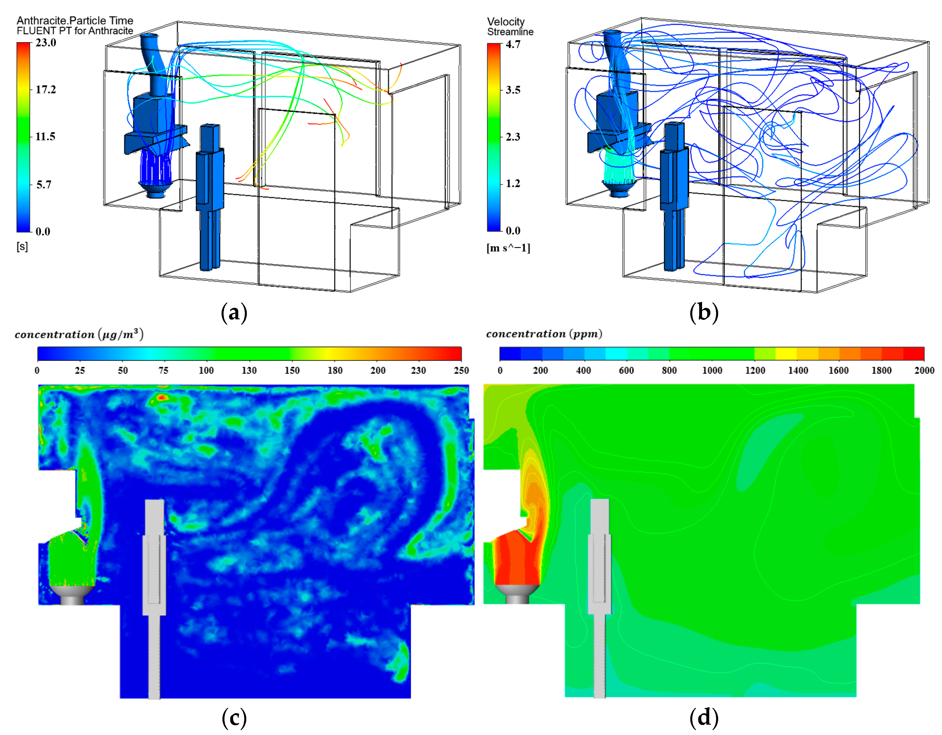
3.2. Simulation Process of COFP and CO2

In the present study, we utilized the temperature data measured at 300 locations above the cooking pot and established the following virtual cooking heat source mode through a self-developed UDF program, and the test data and comparison between test data and simulation results are shown in Figure 7.
T ( x , y , z , t ) f l   0 t < 30 ,   200 t < 300 2 t 3 + f l 20   30 t < 45 8 t 135 + f l + 198 27   45 t < 180 9 t 10 + f l + 180   180 t < 200
f l = 3 x 210 2 + y 1560 2 9409 + 317
V t = 1.5   0 t < 180 3 40 x + 15   180 t < 200 0   200 t < 300
where T ( x , y , z , t ) is the change in temperature over time along the longitudinal direction, f l is the change in temperature along the transverse coordinate, and V t is the velocity of change over time.
In addition, the above model is also used to simulate and calculate the concentrations of COFP and CO2 under the same operating conditions. The parameters of the computational material model employed are given in Table 2 [19]. The total simulation time is 300 s [20]. Based on the test data, the initial temperature of the computational domain is set to 301 K, the speed of the COFP at the surface of the pot is 1.5 m/s, the door gap adopts the equilibrium pressure boundary, and the outlet of the COFP is set as a negative pressure boundary. The details are shown in Table 3. In the computational model described in this study, the human body surface is used as a heat source with a heat flux of 58.12   W / m 2 , while other walls are treated as adiabatic boundaries. For the cooking pot surface, a virtual cooking heat source model is employed.
Depending on the characteristics of the research subject, it is necessary to adjust the physical model and corresponding boundary conditions to ensure the applicability and accuracy of the model. In this study, we use the discrete particle trajectory model to simulate COFP [9]. The model is based on the Euler–Lagrange framework, which can describe the interaction between discrete and continuous phases. It tracks the motion trajectories of multiple particles to obtain information about their distribution and movement. In this study, the total mass flow rate of particles is set to be 2.8 × 10⁻⁸ kg/s [21,22] and the particle diameter is 10 × 10−6 m (PM10) [23]. The particles are uniformly introduced into the calculation domain in the form of a source during the cooking process. The particles can be captured by the human face and arms, while the door cracks and the fume outlet serve as the escape routes for the particles. All other walls are considered as the surfaces where the particles bounce back. In addition, the component transport model that can describe the diffusion and transport behavior of CO2 for the simulation calculation of cooking CO2 is adopted. Within the calculation domain, the initial temperature is 301 K, and the initial concentration of CO2 is 600.21 ppm. The emission of CO2 from cooking noodles depends on the state of the gas stove switch, as shown in Figure 8.

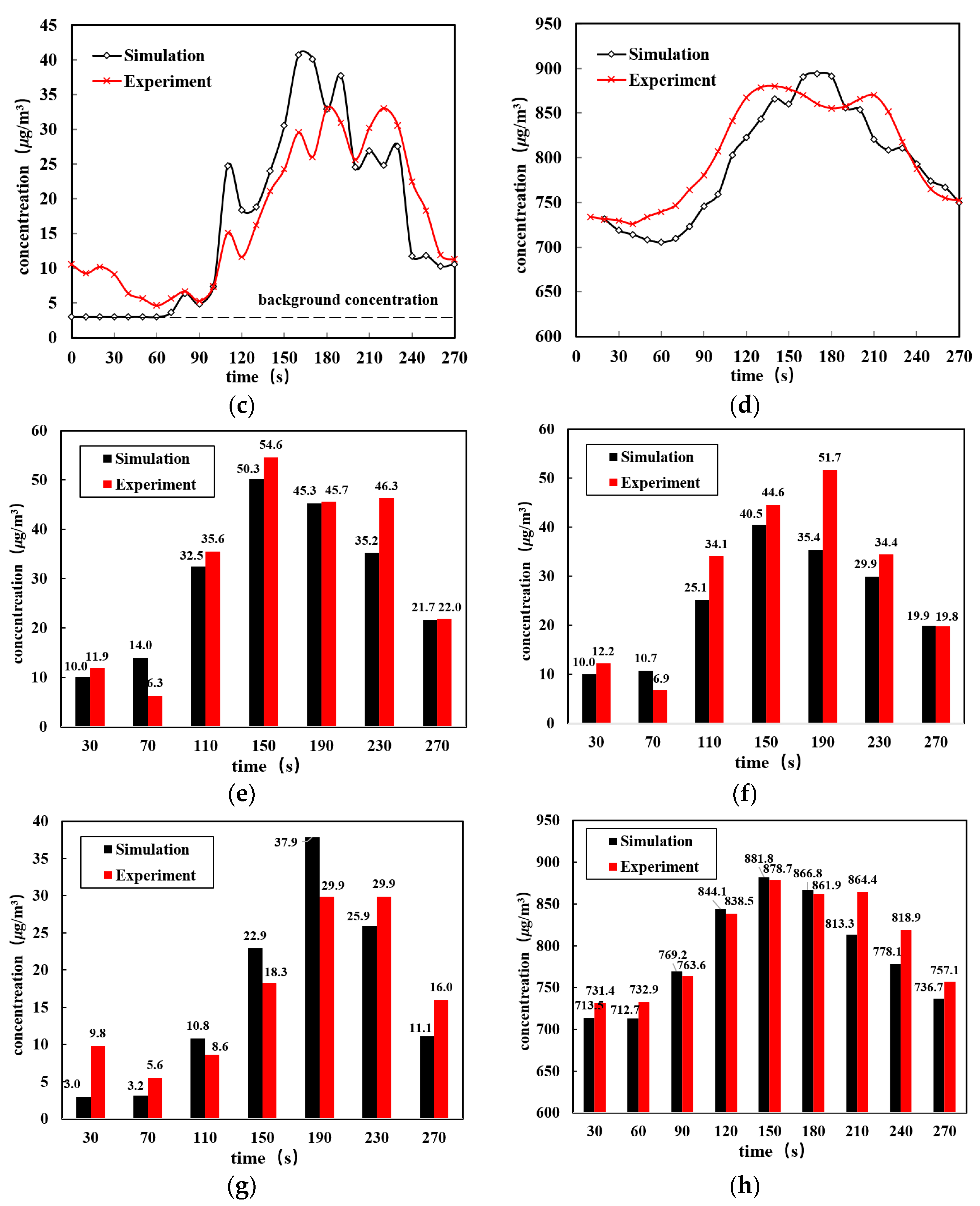
4. Comparison and Analysis of Simulation and Testing

This article processed and analyzed the experimental data and simulation data based on the instrument principles. As can be seen from Figure 9, the simulation results of COFP concentration and CO2 concentration are basically consistent with the experimental results. It can be found that the change in these two pollutants significantly increases from 90 s to 150 s after cooking starts by observing the curves of particle concentration and CO2 concentration over time, which may have a more significant impact on human health.
Within 40 s after the cooking process ended, the experimenters conducted disruptive behaviors such as tidying up and preparing for the next cooking session, which may have a negative impact on the consistency between experimental data and simulation data, thus introducing errors. By observing the concentration histogram of COFP, it is evident that during this period of time, due to the experimenter’s actions, particles on the right side of the face were blown towards the left. Based on the observations of the concentration histogram of COFP, it is apparent that there was a discernible displacement of particles towards the left side of the face during the specific time interval due to the actions of the experimenter. This behavior resulted in the simulated value of P 1 on the right side being higher than the experimentally measured value, while the simulated value of P 2 on the left side was lower than the experimentally measured value.

5. Study on the Substitutability of COFP

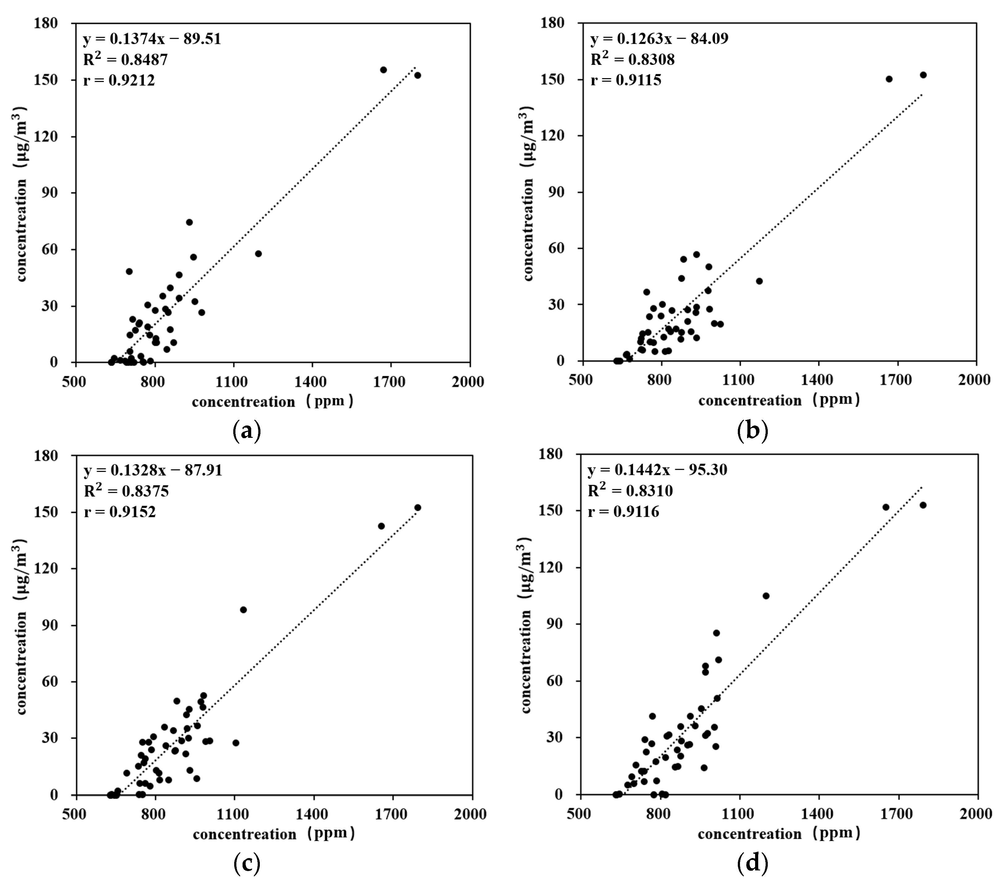
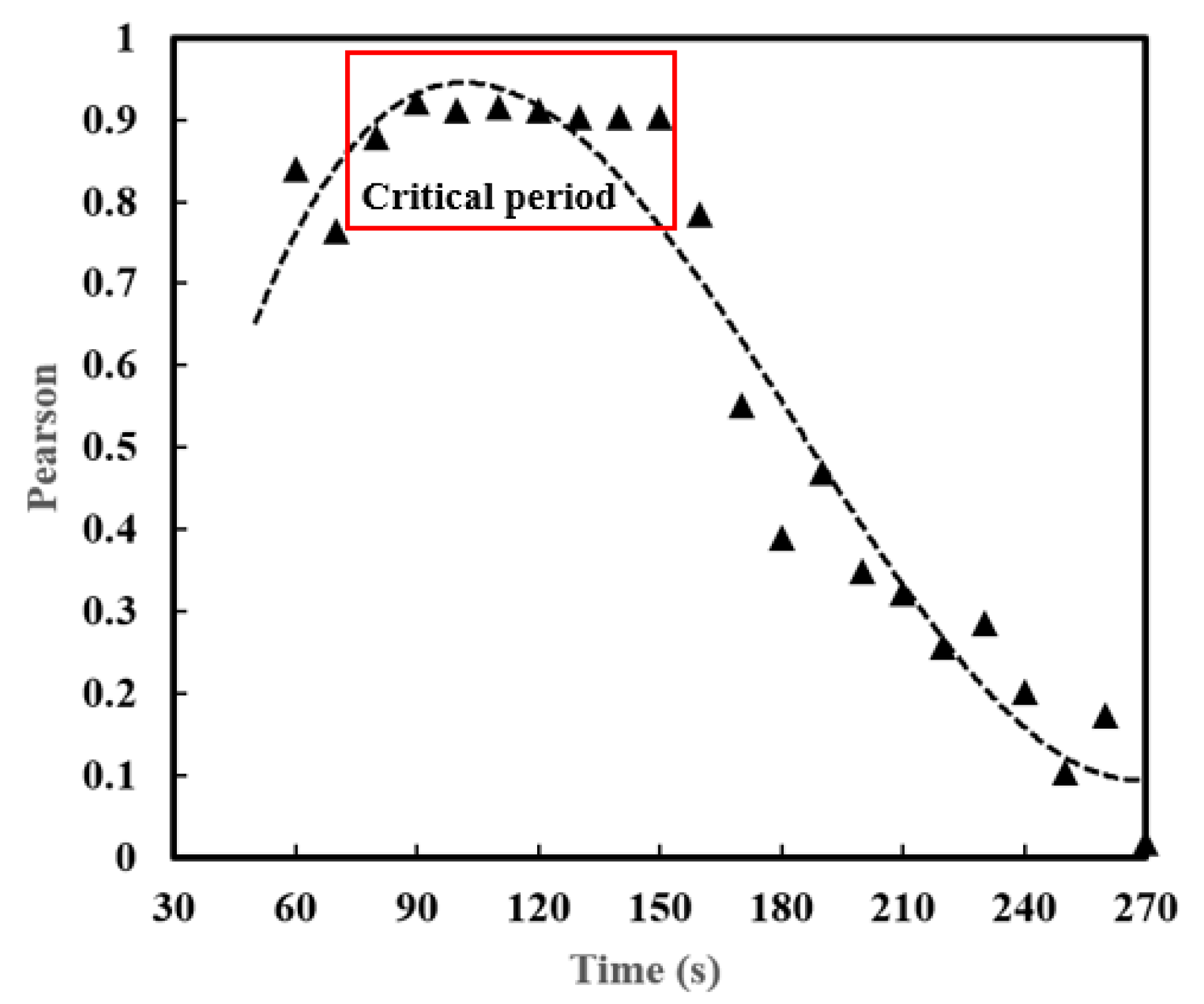
5.1. Analysis of the Correlation between COFP and CO2

It is essential to study particles during the cooking process, but there are certain limitations in the experimental testing [24]. To begin with, due to the temporal and spatial variations experienced by particles during the cooking process, single-point monitoring is insufficient for providing a comprehensive understanding of their overall changes. Secondly, specialized equipment and technical support are required because of the high level of experimental complexity and expense involved in particle research. Although numerical calculations can effectively reduce the cost of simulating COFP, this method requires a large amount of computer resources and time, and it cannot achieve efficient and rapid analysis and control.
Based on the simulation results of this study, it can be observed in Figure 10 that the smaller the gas continuous phase velocity, the longer the particle discrete phase retention time and this results in similar concentration distribution characteristics of CO2 and COFP generated during cooking [25]. Furthermore, we also found that the computer resources required for simulating cooking processes using CO2 were lower compared to simulating COFP (Table 4), resulting in a 70% increase in efficiency. Consequently, this study utilized numerical calculation methods to investigate the spatial distribution characteristics of CO2 and COFP during cooking, thus exploring the feasibility of using CO2 as a substitute for COFP.
According to the testing and simulation results, it was shown that the concentration of COFP and CO2 rapidly rose and peaked during the period of 90 to 150 s after the start of cooking, with a significant increase in amplitude. This indicates that the impact of these two pollutants on human health may be more pronounced during this time period. Therefore, it would be interesting to carry out a correlation analysis between the distribution of COFP concentration around the human body and the CO2 concentration distribution during the critical period of cooking (Figure 11).
To further investigate the spatial correlation between COFP and CO2, we extracted the data from 48 monitoring points during the critical period. These monitoring points were located in close proximity to the human body, spaced 400 units apart from each other, with distances of 400, 800, 1200, and 1600 units from the ceiling. Their specific locations are detailed in Figure 12. Firstly, a scatter plot of the COFP concentration and CO2 concentration is generated using the extracted data and followed by conducting correlation analysis using Pearson correlation [26]. Subsequently, a linear regression analysis using the least square method is employed to fit the COFP concentration and CO2 concentration under the same operational conditions [27], that is,
r = i = 1 n x i x ¯ y i y ¯ i = 1 n x i x ¯ 2 i = 1 n y i y ¯ 2
where r is the Pearson correlation coefficient, and x ¯ and y ¯ are the mean values of the data, respectively.

5.2. Correlation Analysis Results

The correlation between COFP and CO2 concentrations are analyzed by using the data obtained from Figure 13 and Figure 14. From the figures, it is evident that there is a noticeable correlation between the concentration of COFP and CO2 over time. This correlation exhibits a pattern of initially increasing and then decreasing, and is closely tied to cooking activities. Once cooking ceases, the concentration distributions of COFP and CO2 tend to differentiate due to their distinct sedimentation rates and diffusion characteristics. Thus, COFP and CO2 gradually segregate in the air as time elapses, leading to varying concentration distributions across different regions. To be more specific, it is found in Figure 13 that cooking activities exerted an influence on the generation and movement trajectories of both pollutants during the critical period. The results demonstrate a strong correlation (Pearson correlation coefficient (r > 0.9) between the concentrations of COFP and CO2 in the ambient air surrounding the human body under the same heat flow conditions. This suggests that there exists a linear relationship between the concentrations of COFP and CO2. The linear regression equation can be used to fit this relationship, with a high coefficient of determination (R2 > 0.8), indicating that the regression model can explain over 80% of the variance in the data. Therefore, within a specific time period, this study suggests that the concentration distribution of COFP during cooking can be partially reflected by measuring the distribution of CO2 concentration around the human body. This method has a certain degree of feasibility and application prospect, which is of great significance for the research in air pollution and indoor environment monitoring, as well as related fields.

5.3. The Relationship Functions

One of the main objectives of this study is to achieve rapid analysis and control of COFP concentration through low-cost CO2 analysis and monitoring. To this end, we construct a relationship function between COFP concentration and CO2 concentration during the critical period (90~150 s) using the coefficient weighted averaging method (Equation (10)). Subsequently, the final relationship function between the two is obtained (Equation (11)) by correcting the temporal variations of COFP concentration and CO2 concentration in the space near the human body.
a = i n a i r i i n r i
y = 0.136 x 93
By using the relationship function between COFP concentration and CO2 concentration, we can correct the simulated results of CO2 concentration during cooking and obtain the modified distribution characteristics of C O F P c o 2 concentration. In order to verify the rationality of the relationship function, a comparative analysis of the simulated results of COFP and C O F P c o 2 under the same conditions is conducted. The corresponding results are shown in Table 5, which indicate that the absolute error between the two simulated results is less than 5 μ g / m 3 and the corresponding accuracy exceeds 90% under the same conditions, which demonstrates that the relationship function is reliable and can be used to predict the concentration of COFP by predicting the concentration of CO2.

6. Conclusions

This study employed a combined method of Fluent CFD analysis and experimental testing to deeply investigate the spatiotemporal distribution characteristics of COFP and CO2 generated during a kitchen cooking process. On this basis, a relationship function is constructed between them by analyzing the correlation between CO2 and COFP. The simulated results of CO2 are obtained from the relationship function, which can replace the simulated results of COFP with an accuracy of over 90%. The specific contents of this paper include three aspects:
(1)
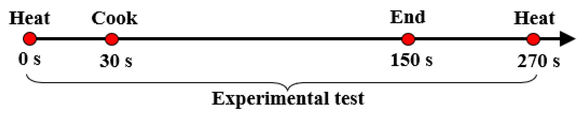
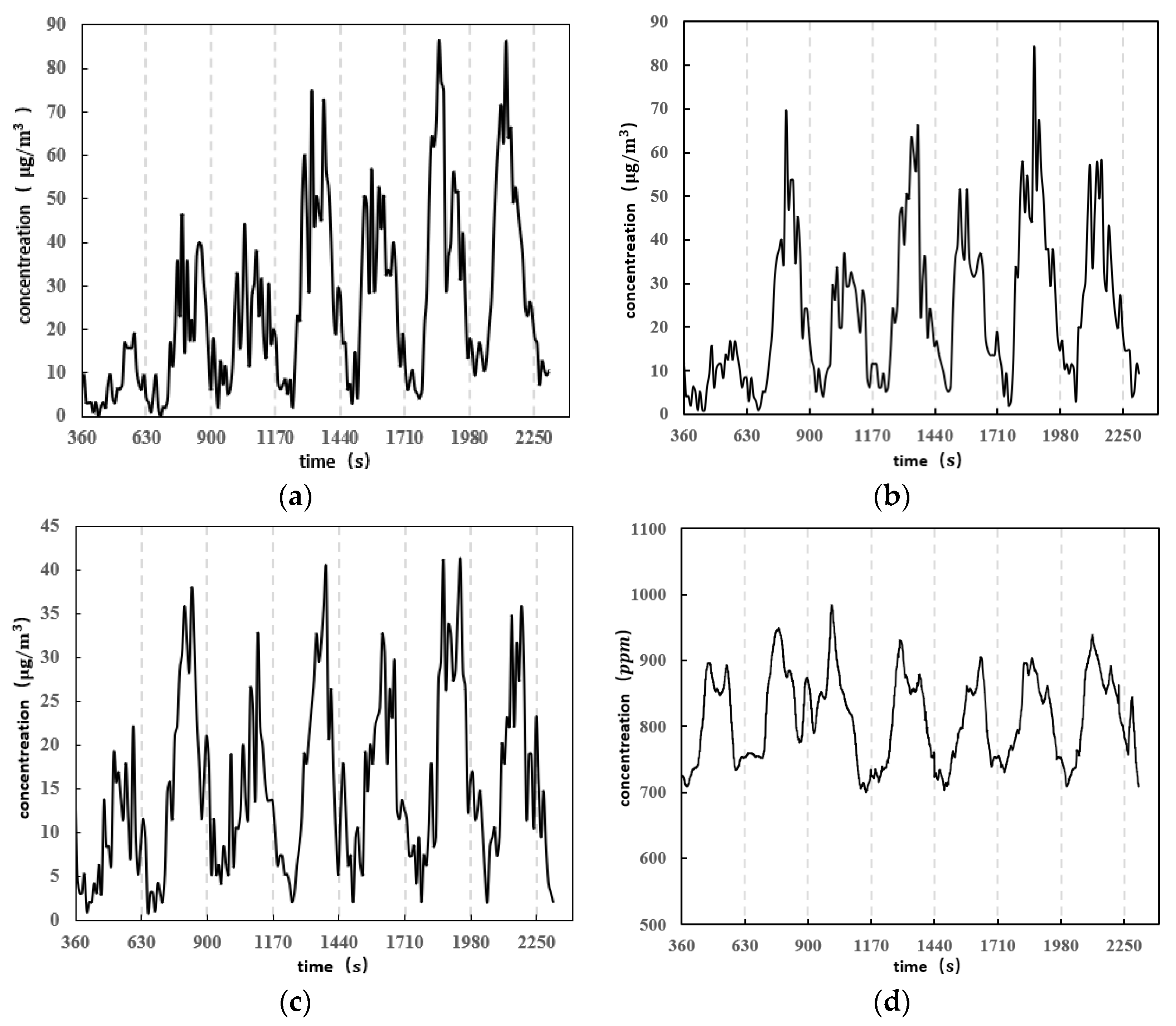
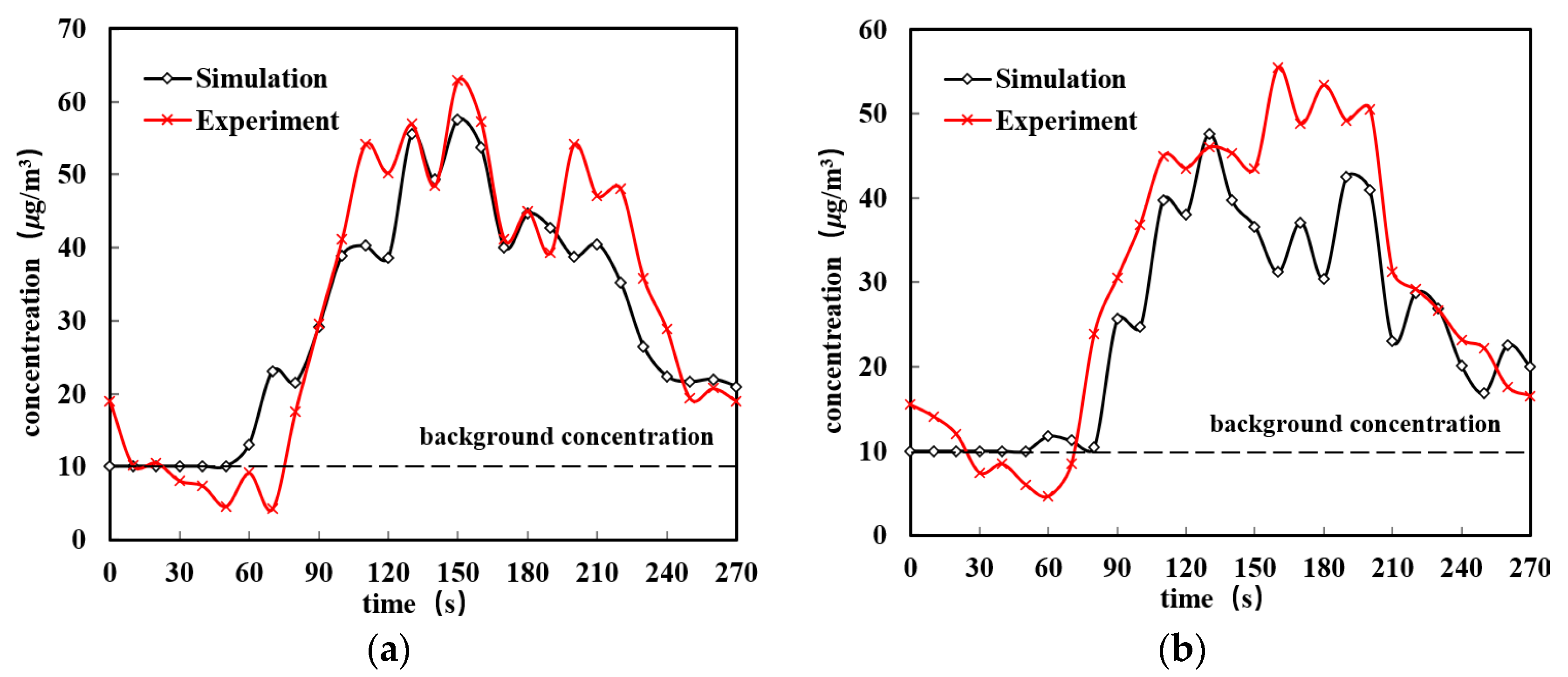
A kitchen experiment testing platform was set up to monitor and collect the concentrations of COFP and CO2 during multiple identical cooking processes. By organizing and analyzing the experimental data, it was found that the concentrations of COFP and CO2 would sharply increase after 90 s of cooking and reach their peak at the end of the cooking process (150 s). Moreover, the time of concentration peak was observed to be delayed with the decrease in spatial height.
(2)
We utilized the same kitchen grid model and developed simulation processes for COFP and CO2 during cooking through the discrete phase model and the species transport model. The boundary conditions were built by using UDF to simulate the movement and diffusion of COFP and CO2 under the same operating conditions. The reliability of the numerical simulation process was validated by comparing the simulation results with experimental data.
(3)
We propose a method for evaluating and controlling COFP concentration using low-cost CO2 analysis and monitoring technology. Firstly, Pearson correlation theory and the linear fitting method were used to analyze and organize the data. The results showed that there was a strong correlation (r > 0.9) between the concentration of COFP and CO2 concentration during the critical cooking period (90~150 s), and more than 80% of the variability could be explained by the linear model. Based on this, the coefficient-weighted averaging method was used to construct a relationship function between COFP concentration and CO2 concentration. The CO2 simulation correction result obtained from this can replace the COFP simulation result with an accuracy of over 90%, leading to an increased computation efficiency of 70%.

Author Contributions

M.D. conducted numerical simulation calculations in the cooking environment, S.Z. conducted data processing and analysis, J.W. conducted on-site testing of the cooking environment, F.Y. conducted experimental testing design, and Z.C. drafted a manuscript. All contributors who do not meet the criteria for authorship should be listed in an acknowledgements section. All authors have read and agreed to the published version of the manuscript.

Funding

This research received no external funding.

Institutional Review Board Statement

Not applicable.

Informed Consent Statement

Informed consent was obtained from all subjects involved in the study. Written informed consent has been obtained from the patient(s) to publish this paper.

Data Availability Statement

Information and data used in the study will be provided upon reasonable request.

Acknowledgments

We would like to thank the Zhejiang Province Public Welfare Technology Application Research Project (LGG22E080020) and 2025 Major Programs on Science Technology Innovation of Ningbo (2020Z06) for their support for this research.

Conflicts of Interest

The authors declare that they have no known competing financial interest or personal relationships that could have appeared to influence the work reported in this paper.

References

  1. Leikauf, G.D.; Kim, S.H.; Jang, A.S. Mechanisms of ultrafine particle-induced respiratory health effects. Exp. Mol. Med. 2020, 52, 329–337. [Google Scholar] [CrossRef] [PubMed]
  2. Xue, T.; Han, Y.; Fan, Y.; Zheng, Y.; Geng, G.; Zhang, Q.; Zhu, T. Association between a Rapid Reduction in Air Particle Pollution and Improved Lung Function in Adults. Ann. Am. Thorac Soc. 2021, 18, 247–256. [Google Scholar] [CrossRef] [PubMed]
  3. Wong, Y.J.; Shiu, H.Y.; Chang, J.H.; Ooi, M.C.G.; Li, H.H.; Homma, R.; Nik Sulaiman, N.M. Spatiotemporal impact of COVID-19 on Taiwan air quality in the absence of a lockdown: Influence of urban public transportation use and meteorological conditions. J. Clean. Prod. 2022, 365, 132893. [Google Scholar] [CrossRef] [PubMed]
  4. Kumar, S.; Jain, M.K. Interrelationship of Indoor Particulate Matter and Respiratory Dust Depositions of Women in the Residence of Dhanbad City, India. Environ. Sci. Pollut. Res. Int. 2022, 29, 4668–4689. [Google Scholar] [CrossRef]
  5. Tong, X.; Ho, J.M.W.; Li, Z.; Lui, K.H.; Kwok, T.C.Y.; Tsoi, K.K.F.; Ho, K.F. Prediction model for air particulate matter levels in the households of elderly individuals in Hong Kong. Sci. Total Environ. 2020, 717, 135323. [Google Scholar] [CrossRef] [PubMed]
  6. Shupler, M.; Hystad, P.; Birch, A.; Chu, Y.L.; Jeronimo, M.; Miller-Lionberg, D.; Brauer, M. Multinational prediction of household and personal exposure to fine particulate matter (PM2.5) in the PURE cohort study. Environ. Int. 2022, 159, 107021. [Google Scholar] [CrossRef] [PubMed]
  7. Kim, Y.; Shin, D.; Hong, K.J.; Lee, G.; Kim, S.B.; Park, I.; Hwang, J. Prediction of indoor PM2.5 concentrations and reduction strategies for cooking events through various IAQ management methods in an apartment of South Korea. Indoor Air 2022, 32, e13173. [Google Scholar] [CrossRef] [PubMed]
  8. Wang, D.; Li, Q.; Shen, G.; Deng, J.; Zhou, W.; Hao, J.; Jiang, J. Significant ultrafine particle emissions from residential solid fuel combustion. Sci. Total Environ. 2020, 715, 136992. [Google Scholar] [CrossRef]
  9. Xiang, J.; Hao, J.; Austin, E.; Shirai, J.; Seto, E. Characterization of cooking-related ultrafine particles in a US residence and impacts of various intervention strategies. Sci. Total Environ. 2021, 798, 149236. [Google Scholar] [CrossRef]
  10. Zhou, Y.; Yang, G. A predictive model of indoor PM2.5 considering occupancy level in a hospital outpatient hall. Sci. Total Environ. 2022, 844, 157233. [Google Scholar] [CrossRef]
  11. Lai, A.C.K.; Chen, F.Z. Comparison of a new Eulerian model with a modified Lagrangian approach for particle distribution and deposition indoors. Atmos. Environ. 2007, 41, 5249–5256. [Google Scholar] [CrossRef] [PubMed]
  12. Kim, H.; Kang, K.; Kim, T. CFD Simulation Analysis on Make-up Air Supply by Distance from Cookstove for Cooking-Generated Particle. Int. J. Environ. Res. Public Health 2020, 17, 7799. [Google Scholar] [CrossRef]
  13. Zhao, B.; Yang, C.; Yang, X.; Liu, S. Particle dispersion and deposition in ventilated rooms: Testing and evaluation of different Eulerian and Lagrangian models. J. Build. Environ. 2007, 43, 388–397. [Google Scholar] [CrossRef]
  14. Gao, N.P.; Niu, J.L.; Perino, M.; Heiselberg, P. The airborne transmission of infection between flats in high-rise residential buildings: Particle simulation. Build. Environ. 2009, 44, 402–410. [Google Scholar] [CrossRef] [PubMed]
  15. Hong, B.; Qin, H.; Jiang, R.; Xu, M.; Niu, J. How Outdoor Trees Affect Indoor Particulate Matter Dispersion: CFD Simulations in a Naturally Ventilated Auditorium. Int. J. Environ. Res. Public Health 2018, 15, 2862. [Google Scholar] [CrossRef]
  16. Tan, H.; Wong, K.Y.; Othman, M.H.D.; Kek, H.Y.; Wahab, R.A.; Ern, G.K.P.; Lee, K.Q. Current and potential approaches on assessing airflow and particle dispersion in healthcare facilities: A systematic review. Environ. Sci. Pollut. Res. Int. 2022, 29, 80137–80160. [Google Scholar] [CrossRef] [PubMed]
  17. Abdolzadeh, M.; Alimolaei, E.; Pustelnik, M. Numerical simulation of airflow and particle distributions with floor circular swirl diffuser for underfloor air distribution system in an office environment. Environ. Sci. Pollut. Res. Int. 2019, 26, 24552–24569. [Google Scholar] [CrossRef] [PubMed]
  18. Chen, R.; You, X.Y. Effects of chef operation on oil fume particle collection of household range hood. Environ. Sci. Pollut. Res. Int. 2020, 27, 23824–23836. [Google Scholar] [CrossRef]
  19. Chen, Z.; Xin, J.; Liu, P. Air quality and thermal comfort analysis of kitchen environment with CFD simulation and experimental calibration. J. Build. Environ. 2020, 172, 106691. [Google Scholar] [CrossRef]
  20. Wong, K.Y.; Tan, H.; Nyakuma, B.B.; Kamar, H.M.; Tey, W.Y.; Hashim, H.; Kuan, G. Effects of medical staff’s turning movement on dispersion of airborne particles under large air supply diffuser during operative surgeries. Environ. Sci. Pollut. Res. Int. 2022, 29, 82492–82511. [Google Scholar] [CrossRef]
  21. Zhao, Y.; Zhao, B. Emissions of air pollutants from Chinese cooking: A literature review. Build. Simul. 2018, 11, 977–995. [Google Scholar] [CrossRef]
  22. Zhao, Y.; Chen, C.; Zhao, B. Emission characteristics of PM2.5-bound chemicals from residential Chinese cooking. Build. Environ. 2019, 149, 623–629. [Google Scholar] [CrossRef]
  23. Lai, A.C.K.; Ho, Y.W. Spatial concentration variation of cooking-emitted particles in a residential kitchen. J. Build. Environ. 2008, 43, 871–876. [Google Scholar] [CrossRef]
  24. Chang, T.J.; Hsieh, Y.F.; Kao, H.M. Numerical investigation of airflow pattern and particulate matter transport in naturally ventilated multi-room buildings. Indoor Air 2006, 16, 136–152. [Google Scholar] [CrossRef] [PubMed]
  25. Shen, H.; Hou, W.; Zhu, Y.; Zheng, S.; Ainiwaer, S.; Shen, G.; Tao, S. Temporal and spatial variation of PM2.5 in indoor air monitored by low-cost sensors. Sci. Total Environ. 2021, 770, 145304. [Google Scholar] [CrossRef] [PubMed]
  26. Jung, C.C.; Lin, W.Y.; Hsu, N.Y.; Wu, C.D.; Chang, H.T.; Su, H.J. Development of Hourly Indoor PM2.5 Concentration Prediction Model: The Role of Outdoor Air, Ventilation, Building Characteristic, and Human Activity. Int. J. Environ. Res. Public Health 2020, 17, 5906. [Google Scholar] [CrossRef] [PubMed]
  27. Cho, S.; Lee, G.; Park, D.; Kim, M. Study on Characteristics of Particulate Matter Resuspension in School Classroom through Experiments Using a Simulation Chamber: Influence of Humidity. Int. J. Environ. Res. Public Health 2021, 18, 2856. [Google Scholar] [CrossRef]
Figure 1. Experimental kitchen.
Atmosphere 14 01522 g001
Figure 2. Geometric model and arrangement of monitoring points (all dimension units are mm). (a) Geometric model; (b) arrangement of monitoring points.
Atmosphere 14 01522 g002
Figure 3. Experimental testing process.
Atmosphere 14 01522 g003
Figure 4. Variation of concentration of COFP and CO2 with time. (a) P1; (b) P2; (c) P3; (d) Pc.
Atmosphere 14 01522 g004
Figure 5. Grid sensitivity analysis.
Atmosphere 14 01522 g005
Figure 6. Mesh of the computational domain.
Atmosphere 14 01522 g006
Figure 7. Test data and comparison between test data and simulation results. (a) Temperature test data; (b) curve of temperature data comparison over time; (c) wind speed test data; (d) curve of wind speed data comparison over time.
Atmosphere 14 01522 g007
Figure 8. Variation of concentration of CO2 sources with time.
Atmosphere 14 01522 g008
Figure 9. Comparison of simulation results and experimental results. (a) Curve of P 1 data comparison over time; (b) curve of P 2 data comparison over time; (c) curve of P 3 data comparison over time; (d) curve of P c data comparison over time; (e) histogram of P 1 data comparison over time; (f) histogram of P 2 data comparison over time; (g) histogram of P 3 data comparison over time; (h) histogram of P c data comparison over time.
Atmosphere 14 01522 g009aAtmosphere 14 01522 g009b
Figure 10. COFP and CO2 streamlines and distribution characteristics. (a) Streamlines of PM10; (b) streamlines of CO2; (c) distribution of PM10; (d) distribution of CO2.
Atmosphere 14 01522 g010
Figure 11. Experiment process.
Atmosphere 14 01522 g011
Figure 12. Arrangement monitoring points.
Atmosphere 14 01522 g012
Figure 13. Correlation between COFP concentration and CO2 concentration at different time points. (a) 90 s; (b) 100 s; (c) 110 s; (d) 120 s; (e) 130 s; (f) 140 s; (g) 150 s; (h) 180 s.
Atmosphere 14 01522 g013aAtmosphere 14 01522 g013b
Figure 14. Pearson correlation coefficient change over time.
Atmosphere 14 01522 g014
Table 1. Test parameters.
Parameters
Initial temperature at the center of the pot surface (°C)200
Heating time (s)30
Temperature to which the center of the pot surface is heated (°C)230~240
Weight of potatoes (g)300 ± 2
Weight of sunflower oil (g)14.5 ± 0.5
Stirring methodlower right, down, left (clockwise)
Interval between stirring (s)1
Cooking time (s)120
Cooling time (s)120
Testing cycle (s)270
Testing time (s)2250 – 270 – 90 = 1890
Table 2. Material parameters.
L i q u i d   P r o e r t y
A i r d e n s i t y   ( g / m 3 ) 1.225
A i r t h r m a l c o n d u c t i v i t y   ( W / m · K ) 0.0242
A i r v i s c o s i t y   ( k g / m · s ) 1.7894 × 10⁻⁵
C O 2 d e n s i t y   ( k g / m 3 ) 1.7878
C O 2 t h r m a l c o n d u c t i v i t y   ( W / m · K ) 0.0145
C O 2 v i s c o s i t y   ( k g / m · s ) 1.37 × 10⁻⁵
S o l i d p r o e r t y
S o l i d d e n s i t y   ( k g / m 3 ) 950
S o l i d t h e r m a l c o n d u c t i v i t y   ( W / m · K ) 0.33
S o l i d d i a m e t e r   ( m ) 1 × 10⁻⁵
Table 3. Boundary conditions for CFD simulation.
BoundaryBoundary ConditionValue
Virtual heat source moduleVelocity inlet Surface   temperature :   T   ( x , y , z , t )
Velocity :   V   ( t )
Range hood outletPressure outletSurface temperature: 293 K
Pressure: −5.7 Pa
Door gapPressure inletSurface temperature: 298 K
Pressure: 0.0 Pa
Human bodyWall (heat source)Heat: 16 W/m2
Table 4. Computer and calculation parameters.
Computer Parameter
ProcessorDual-core processor
CPU core48
Thread96
Calculation parameter
Calculation MethodParallel Computing
Thread36
Simulated Cooking COFP Time240 h
Simulated Cooking CO2 Time72 h
Table 5. Comparison of average data of 48 points in space near human body.
Work ConditionCOFP
( μ g / m 3 )
C O F P C O 2
( μ g / m 3 )
Absolute Error
( μ g / m 3 )
Relative Error
95 s23.9824.290.311.29%
105 s28.9227.15−1.77−6.12%
115 s27.5029.341.846.69%
125 s33.6930.61−3.08−9.14%
135 s31.0831.710.632.01%
145 s34.3933.55−0.85−2.46%
Disclaimer/Publisher’s Note: The statements, opinions and data contained in all publications are solely those of the individual author(s) and contributor(s) and not of MDPI and/or the editor(s). MDPI and/or the editor(s) disclaim responsibility for any injury to people or property resulting from any ideas, methods, instructions or products referred to in the content.

