Article

CO2, CH4, and CO Emission Sources and Their Characteristics in the Lamto Ecological Reserve (Côte d’Ivoire)

by
Dro Touré Tiemoko
1,2,*,
Fidèle Yoroba
2,3,
Komenan Benjamin Kouassi
2,3,
Adama Diawara
2,3,
Kouakou Kouadio
2,3,
Francois-Xavier Djezia Bella Bouo
1,
Assi Louis Martial Yapo
2,4,
Abraham Kouman
3 and
Michel Ramonet
5
1
Equipe de la Physique pour l’Environnement, Laboratoire de Physique Fondamentale et Appliquée, Université Nangui Abrogoua, Abidjan 02 BP 801, Côte d’Ivoire
2
Geophysical Station of Lamto (GSL), N’Douci BP 31, Côte d’Ivoire
3
Laboratoire des Structures de la Matière, de l’Environnement et de l’Énergie Solaire (LASMES), Université Felix Houphouët-Boigny, UFR SSMT, Abidjan 22 BP 582, Côte d’Ivoire
4
Department of Sciences and Technology, University Alassane Ouattara, Bouaké 01 BPV 108, Côte d’Ivoire
5
Laboratoire des Sciences du Climat et de l’Environnement (LSCE), IPSL, CEA-CNRS UVSQ, Université Paris-Saclay, Orme des Merisiers, 91191 Gif-sur-Yvette, France
*
Author to whom correspondence should be addressed.
Atmosphere 2023, 14(10), 1533; https://doi.org/10.3390/atmos14101533
Submission received: 29 July 2023 / Revised: 11 September 2023 / Accepted: 14 September 2023 / Published: 6 October 2023
(This article belongs to the Section Climatology)

Abstract

:
CO2, CH4, and CO are the most critical atmospheric gases in terms of their impact on the radiative system, air quality, and health. This work provides information on the direction of source areas and potential sources of emissions and shows many aspects of these gases by a statistical analysis using bivariate polar diagrams and local weather conditions (e.g., temperature, wind speed, and wind direction), recorded at the Lamto station (LTO, 6°31′ N and 5°2′ W) in Côte d’Ivoire over the 2014–2018 period. The results show that the main regions contributing to the high concentrations of CH4 (>1925 ppb) and CO2 (>420 ppm) in the great dry season (GDS), great wet season (GWS), short dry season (SDS), and short wet season (SWS) are the north and north-west sectors of Lamto. In these directions, CH4 and CO2 concentrations are associated with wind speeds less than 6 m.s−1, due to the influences of local sources as emissions resulting from the degradation of organic matter submerged during the impoundment of the Taabo dam, and/or human activities linked to the practice of intensive agriculture. In addition, the high concentrations of CO (>350 ppb) are observed in GDS in the north, north-west, north-east, and east sectors for wind speeds less than or equal to 9 m.s−1, due to the influences of both local and distant sources. The correlation coefficients between CH4 and CO and between CH4 and CO2 are positive and significant in all sectors. However, those calculated between CO2 and CO have showed both low and high values in all seasons.

1. Introduction

In atmospheric science, the study of the relationships between CO2, CH4, and CO and meteorological parameters on the one hand, and correlation and comparison techniques on the other hand, are very useful. These techniques allow for identifying and characterizing the various sources of these gases [1] and controlling trends through their emission. Moreover, to better distinguish these emission sources, it is necessary to characterize their spatial and temporal distributions. For this purpose, analyzing the wind speed and direction at small and large scales, as well as turbulence and atmospheric stability responsible for the dispersion of the gaseous compounds, is important. The emission processes of these gases are also dependent on ambient (or local) weather conditions because they are influenced by short-wave radiation, temperature, humidity, etc. [2,3,4].
The correlation between pairs of gases also leads to characterizing emission sources rather than studying slopes from regression diagrams [5]. Indeed, Manoli et al. [6] underlined that the analyses derived from the use of simple and static slopes could not be suitable in many situations. In addition, some simple analysis techniques (e.g., boosted regression trees, concentration weighted trajectory (CWT), etc.) and identifications (e.g., non-parametric wind regression (NWR), potential source contribution function (PSCF)) are used and provide important information on sources that are difficult to characterize. The modeling of the receivers is also used very frequently because it takes into account several aspects, for example, the radiative and boundary layer processes, etc.
This modeling technique has the advantage of identifying and characterizing the emission sources of CO2, CH4, and CO. However, given the complexity of some boundary layer processes such as convection and/or turbulence, the air quality models sometimes have a difficulty in providing information that allows for better identifying and characterizing emission sources. As a result, in situ data analysis remains one of the most adequate approaches. Some studies [7,8,9] have shown that through an innovative technique application on in situ data, this approach allows for collecting more information. One of these techniques is to statistically analyze the atmospheric concentration levels of species by clustering footprints calculated with the FLEXPART model [10,11,12]. This technique allows (1) for characterizing the role of long-range atmospheric transport of air masses and quantifying its impact on the variability of synoptic, seasonal, and interannual signals of atmospheric species and (2) establishing source–receptor relationships. Applying this approach on CO2, CH4, and CO concentrations measured at Lamto over the 2014–2018 period, Tiemoko et al. [12] have shown that high concentrations of these species were observed when the air masses coming exclusively from north-east and North Africa transited through some West African countries (Ghana, Togo, Benin, Nigeria, Niger, Burkina-Faso). These authors have shown that these continental emissions explain ~40%, ~74%, and ~66% of the variances of CO2, CH4, and CO, respectively. The results of this study have led to specific conclusions and highlighted the impacts of distant emission sources. However, in order to explain the totality of the CO2, CH4, and CO variances on the site, it is also necessary to take into account the local impacts such as those resulting from the presence of the Taabo hydroelectric dam near the Lamto station. Indeed, Rosa and Schaeffer. [13], Galy-Lacaux et al. [14,15], and Delmas et al. [16] pointed out that these emissions have proven to be significant in a tropical environment.
These facts here show the necessity of using another innovative technique, which is the bivariate polar diagram [17,18] through the package Openair [19] for the R programming environment. This bivariate method, which takes into account the local meteorological conditions, in particular, wind speed and direction, is effective to determine potential emission directions of the gases and their correlations between each wind sector. It is now widely used by a large part of the scientific community for the air quality and climate change studies [20]. These applications have shown good results in the determination study of the potential emission sources of gases [21,22] and atmospheric pollutants [23,24].
This study aims to analyze the temporal relationships existing between local meteorological parameters and CO2, CH4, and CO, which are known for their significant contributions to radiative forcing [25]. Therefore, we will determine the dominant sources and identify the trends of their variations, as well as the probable causes of the high concentrations measured sometimes at the LTO station over the 2014–2018 period, using the Openair package functions in the R environment.
This work is structured as follows: Section 2 describes the study area, data, and methods used. Section 3 presents the results and discussion. Finally, we conclude and provide some perspectives on future improvements of the work.

2. Material Data and Method
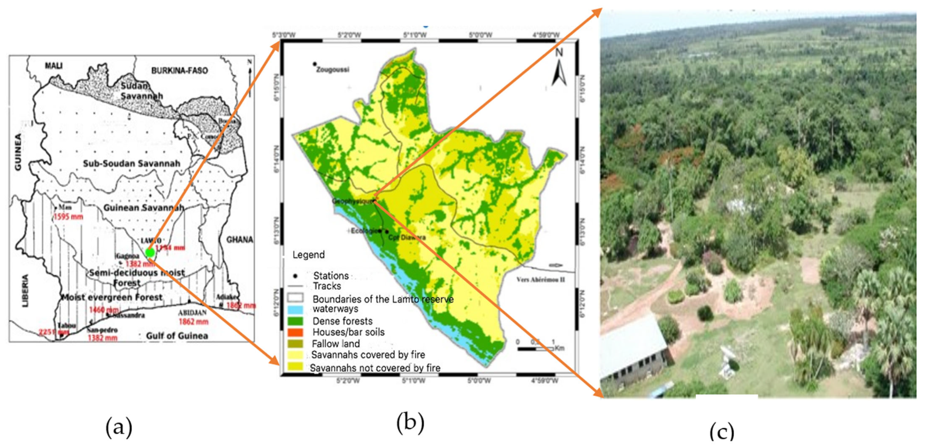
2.1. Study Area

The region of Lamto (5°2′ W and 6°13′ N, Figure 1) is in an equatorial transition climate [26]. Indeed, to simplify, Devineau [27] underlines that the rainfall regime at Lamto is governed by a struggle influence between the monsoon in the south and harmattan in the north. In the confluence area, the moist air (i.e., monsoon) is more or less depressed under the hot and dry air mass (i.e., harmattan). The delimitation zone at the ground between these two air masses is the intertropical front (FIT) and it is inclined from south to north. This front moves from south to north and from north to south during the year in relation to the thermal equator [28] and, at Lamto, it provides a rainfall regime of four seasons (i.e., two rainy seasons and two dry seasons).
The great wet season is from March to July (GWS), while the short wet season is from September to November (SWS). Then, the great dry season appears from December to February (GDS), while the short dry season (SDS) is confined to August. The mean annual rainfall amount and temperature are 1200 mm and 27 °C, respectively. The vegetation is mainly wet savannah (80% of the area) and forest (20% of the area). Anthropogenic activities are those related to agriculture, fishing, and livestock farming. The Lamto region is influenced by annual passes of bush fires destroying about 80% of the aboveground biomass [29].

2.2. Data

The meteorological parameters (ground-base observation), such as temperature and wind speed and direction, as well as CO2, CH4, and CO concentrations used in this work were measured simultaneously over the 2014–2018 period at Lamto. CO2, CH4, and CO concentrations were measured using the CRDS_Picarro_G2401 instrument. This instrument model, based on cavity ring-down spectroscopy, has linear and stable responses, and it is recognized for its high accuracy in measuring the molar fractions of CO2 (ppm), CH4 (ppb) and CO (ppb). At Lamto, CRDS shows accuracies below 0.1 ppm, 0.5 ppb, and 16 ppb for CO2, CH4, and CO measurements, respectively (see Tiemoko et al. [4,12]).
Continuous measurements are calibrated to the international reference scale of the World Meteorological Organization (WMO) using six calibration tanks from the Laboratory of Climate and Environmental Sciences (LSCE). The air analyzed is taken continuously at the top of a 50 m tower. The measuring system, data processing, and calibration strategy are explained by Tiemoko et al. [4,12].

2.3. Methods

2.3.1. Bivariate Polar Plots

Bivariate polar diagrams show how a concentration of a gas varies with both wind speed and direction in polar coordinates [18]. These diagrams have shown their performance in a variety of situations, such as characterization of airport sources and characteristics of dispersion in “canyon” streets (i.e., streets subject to atmospheric releases from traffic) [19]. Wind direction and speed can be very important in discriminating various sources of emission [30]. The diagrams use a useful graphical technique that can provide directional information on sources as well as concentration dependence on wind speed or temperature from polar coordinates [20].
To simplify, the bivariate polar diagrams are constructed in the following way: First, the wind speed, wind direction, and concentrations data are divided into classes of wind speed and direction, and mean concentrations calculated for each class. The wind components are explained by Equation (1):
u = u ¯ sin ( 2 π θ ) ;           v = u ¯ cos ( 2 π θ )
where u ¯ is the mean hourly wind speed and θ is the mean wind direction in degrees with origin of 90° E.

2.3.2. Bivariate CPF Methodology

The conditional probability function (CPF) [31] analyzes the impacts of point sources from different directions and wind speeds. It estimates the probability so that the measured concentration exceeds a fixed threshold for a given wind sector [31,32,33] while determining the direction of the source zones that significantly affect the receptor site [34]. In this study, four wind sectors (i = 90 degrees) were chosen and the threshold values were fixed at the 75th percentile over the entire study period in the four seasons of the Lamto rainfall regime. Here, the threshold percentile choice takes into account the distribution of concentrations as a function of wind speed and direction, and the trend of CO2, CH4 and CO species obtained at Lamto area by Tiemoko et al. [12] over the 2014–2018 period. The CPF function is defined by:
    C P F Δ θ   = m Δ θ / C X n Δ θ
where m   Δ θ is the number of samples or the number of exceeded pollution threshold in the wind sector Δθ, the concentration C is greater than or equal to a threshold value X, and n Δ θ is the total number of samples or the total number of hourly data from the same wind sector Δθ.

3. Results and Discussion

3.1. Local Meteorology

The wind regime (Figure 2) shows a predominance of south and south-west wind sectors during the GWS, SDS, and SWS seasons over the 2014–2018 period. The presence of these winds from the south and south-west sectors shows the significant influence of the monsoon flow in the region. However, in GDS season, the predominant winds are observed in three different sectors (i.e., south, south-west, and north-west). In contrast, Lamto does not show predominant winds in the northeastern sector, where the highest wind speed values are available. North-east winds are characteristic of the harmattan flow in the GDS season [35,36]. Winds from the southwestern sector are the majority and their frequency of occurrence is about 27%.
To compare quantitatively the variation in wind speed over the four seasons, statistics including the hourly average, minimum and maximum values of wind speed are presented in Table 1. The average hourly small-scale wind speeds observed are 2.48, 2.49, 2.55, and 2.21 m. s−1 in GDS, GWS, SDS, and SWS, respectively, indicating the existence of relatively weak advection conditions affecting the Lamto area. Indeed, Adler et al. [37] during the DACCIWA (dynamics–aerosol–chemistry–cloud interactions in West Africa) ground-based field campaign emphasize that advection conditions are considered weak when the average wind speed is inferior to 3 m. s−1. The maximum wind speed was 11.15 m.s−1 in GWS, which was 4%, 15%, and 20% higher than in GDS, SDS, and SWS, respectively. The minimum wind speed was quite similar for all four seasons.
Figure 3 shows the average diurnal cycle of temperature (a), wind speed (b), and wind direction (c) during the four seasons of rain regime (GDS, GWS, SDS, and SWS) over the 2014–2018 period at Lamto. Temperature shows pronounced seasonal diurnal cycles with average amplitudes of ~9.3 °C, 6.6 °C, 5.1 °C, and 6.6 °C in GDS, GWS, SDS, and SWS, respectively (see Table 2). These amplitude values indicate that during GDS, the temperature variations are significantly larger than the other three seasons, which show almost similar diurnal variations. Thus, the high magnitude value observed during the GDS could be due to the fact that this season is subject to favorable conditions for the rapid increase (fires) and decrease (harmattan) in temperature on a diurnal scale. During all the seasons, the average hourly minimum temperature was observed in the early morning (05:00 to 06:00 local time), while the maximum value in the early afternoon (14:00 to 16:00 local time). Moreover, diurnal cycles of wind speed (Figure 3b) show two significant peaks at around 9:00 am and 7:00 pm and minimum values in the early morning (6:00 am to 8:00 am local time) and in the afternoon (1:00 pm to 3:00 pm local time) during the different seasons. The wind speed minimum is in phase with the temperature minimum, while the wind speed maximum occurs about 3 h after the afternoon temperature maximum. As for the amplitude values (Table 2), we observe low and quasi-similar average values, indicating a less significant change from one season to another in wind speed on a diurnal scale. Since the diurnal cycles of wind speed and temperature are quite pronounced during the different seasons, it was evident that the trend of day and night data of CO2 and CH4 that is highly dependent on these environmental parameters at an hourly scale, would be significantly different. In Figure 3c, it clearly appears that the diurnal cycle of wind direction in GDS is well pronounced (Table 2), similar to temperature (Figure 3a). During this season, the minimum value of wind direction is reached between 00:00 and 02:00 local time, which is associated with an average direction between 150 and 162° (south-east), while the maximum observed between 15:00 and 17:00 local time is associated with an average direction between 250° and 260° (south-west). However, GWS, SDS, and SWS show diurnal cycles of wind direction that vary very little from one time of day to another and from one season to another.

3.2. CPF and Bivariate Polar Plots

3.2.1. CH4

Figure 4 shows polar diagrams with two variables (i.e., temperature and wind direction, wind speed and wind direction) and the CPF of CH4 during the four seasons of the rainfall regime (i.e., GDS, GWS, SDS, and SWS) at Lamto. Figure 4a shows that high values of concentrations of CH4 (>1850 ppb) come from the northwestern and northeastern sectors with agricultural areas and the Taabo hydroelectric dam, except for the SDS season for which concentrations are below 1850 ppb. These concentrations are highest during the GDS season, coinciding with the bushfire regime in the region. However, it should be noted that fires in tropical forests tend to produce more carbon monoxide (CO) and CH4 per unit of fuel burned [38]. Frequency and severity of droughts accentuate the occurrence of fire events, and emit large amounts of CH4 into the atmosphere due to incomplete burning of forest biomass [39,40]. During the year, high concentration values are associated with wind speeds less than 6 m.s−1. In addition, the CPF function (Figure 3c) indicates that only 25% of the concentration values above 1906 ppb come mainly from sources of the north-west sector in GWS and SWS, and from all directions in GDS. These emission sources of CH4 are local (i.e., wind speed is <6 m.s−1) and are related to the anthropogenic activities above-mentioned. In the GDS season, these emissions are partly related to harmattan wind fluxes. These winds blow from north to south carrying desert dust [35,36,41] and polluted air masses due to Sahelian biomass fires [41,42]. Tiemoko et al. [12] showed that these harmattan winds in the GDS season significantly contributed to the increased CH4 concentration and explained ~64% of its variance. In addition, the heat maps of CH4 concentrations (Figure 4b) show that the significant concentration values during all seasons (>1970 ppb in GDS, >1925 ppb in GWS, >1850 ppb in SDS, and >1950 ppb in SWS) are recorded in the north-west direction with temperature values between 20 °C and 26 °C. However, at the diurnal scale, a lack of clear and significant correlation between temperature and CH4 concentrations is found. These observations highlight the complexity of the relationships between these two variables. Indeed, Figure 4 shows variable effects of temperature from one season to another. The distributions of the significant values of CH4 concentrations are in no way related to any particular variations in temperature.

3.2.2. CO2

Figure 5a,b show two-dimensional polar views of the CO2 concentrations recorded at Lamto, as a function of wind speed (Figure 5a) and temperature (Figure 5b). Figure 5a shows that the lowest molar fractions of CO2 are recorded in SDS, which is in accordance with the general annual cycle observed in the work of Tiemoko et al. [4] (see Figure 5a of Tiemoko et al. [4]). On the other hand, the significant CO2 concentration values (>420 ppm) are recorded in the GDS, GWS, and SWS seasons, and in the north and north-west directions. In these directions, significant concentration values are associated with wind speeds less than 6 m.s−1, which reflect the influences of local emission sources [41]. A similar study [43] has pointed out that the lower the wind speeds (~5 m.s−1), the higher the concentrations recorded are from local sources. Furthermore, in terms of the contribution of long-range transport, Tiemoko et al. [12] pointed out that continental air flows explain 40% of the variance in CO2 concentration. These different results show that the local and regional influences on air quality in the Lamto region are predominantly from the north, north-east, and north-west sectors, suggesting the main directions of local and regional emission sources. In Figure 4b, it appears clearly that the variations in CO2 concentrations depend on temperature variations in all directions and in all seasons. In addition, significant CO2 concentration values (≥415 ppm) are associated with areas where the temperature is below 27 °C. These observations highlight the effects of the atmospheric boundary layer (ABL) and the photosynthesis and respiration activities of the vegetation in the CO2 concentration levels. Indeed, for low temperatures generally at night, dispersed CO2 plumes are brought down to ground level in stable atmospheric conditions under a contracted boundary layer, which induces an accumulation of emissions from local sources. On the other hand, during the day, the high temperatures contribute to diluting the CO2 concentration levels under an unstable and dilated boundary layer. These observations are also shown in the work of Gu et al. [44] and Tiemoko et al. [3]. Tiemoko et al. [4] reached the same conclusion in the Lamto area over the 2008–2018 period. They observed a strong contrast between daily and nighttime values of CO2. Indeed, these authors showed that the temperature is one of the main factors influencing the carbon dioxide produced by vegetation. This influence is significant on the seasonal concentration and its diurnal variation. The conditional probability function (Figure 5c) shows that the over threshold value at the 75th percentile is 423 ppm. These over thresholds come mainly from sources in the north-west (GDS, GWS, and SWS), north-east (GWS, SWS, and SDS), and south-east (SDS) sectors, corroborating the previous results.

3.2.3. CO

Figure 6a,b show two-dimensional polar distributions of CO concentrations recorded at Lamto, as a function of temperature (Figure 6b) and wind direction (Figure 6a). Thermal maps for CO (Figure 6b) show high concentration values (>225 ppb) in GDS and GWS seasons. In GWS, these significant values are associated with temperatures above 32 °C, while low concentration values (<225 ppb) are related to temperatures below 32 °C. This indicates that the temperature is positively correlated with CO in this season. These observations were also observed from March 12th to April 1st, 2009 in central Christchurch in the middle of the east coast of the Southern Island of New Zealand [45]. This positive correlation between temperature and CO could be attributed to the influences of agricultural activities (i.e., burning) in the area that have an impact on local meteorology. Furthermore, in GDS, significant CO concentrations are observed for all temperature ranges, which would indicate the domestic heating influence and combustion by biomass fires during the season. Indeed, GDS represents the great dry season at Lamto and, in this period, fire regimes are particularly intense [4,26]. In addition, the highest concentrations (>375 ppb) come from the north, north-east, east, and east-south sectors. In SWS and SDS seasons, CO concentrations are below 200 ppb for all temperature ranges. These observations could result from the inactivity of potential CO emission sources. The velocity and wind direction maps (Figure 6a) associated with CO concentrations indicate that the significant concentration values in GDS (>350 ppb) come from the north, north-west, north-east, and east sectors despite the greater wind advection (i.e., prevailing winds) in the south and south-west directions (Figure 2). However, these high concentrations are observed for wind speeds between 1 m.s−1 and 9 m.s−1. These observations suggest the existence of two types of sources. Local sources characterized by wind velocities below 6 m.s−1 and regional sources for wind velocities above 6 m.s−1. Regional sources are probably associated with a harmattan flow plume carrying polluted air masses over long distances, as explained in Section 3.2.1 in the case of CH4 [4]. These concentration hot spots in the GDS season are consistent with those observed in the north-west direction for CH4 and CO2. This suggests that active emission sources in GDS are similar. In addition, CO concentrations vary very slightly depending on the characteristics of the wind (i.e., wind speed and direction) in the SDS and SWS seasons. The significant CO concentrations in GWS season are between 225 and 300 ppb in the south, north, and north-west directions and have a similar distribution to that of GDS. In addition, the seasonal probability function (Figure 6c) at the 75th percentile threshold shows that in GDS and SDS, the high CO concentrations (≥265 ppb) have very significant contributions in the north-west, north-east, and east-south directions. These different seasonal orientations could be due to the seasonal changes in wind fields [46]. On the other hand, GWS and SWS seasons do not contribute to the 75th percentile threshold of CO concentration levels, which is explained by the fact that anthropogenic activities (e.g., agricultural burns, bush fires), which are considered the main source of emissions of CO, are dormant during this period of the year.

3.3. Correlation Statistic

In this work, the correlation statistic is very useful to characterize the behavior of CH4, CO2, and CO gas concentrations emitted in the atmosphere. Similar emission sources or gases that undergo similar chemical and/or physical transformations in the atmosphere present high and significant correlation values [1]. In addition, Fu et al. [47] emphasized the importance of correlation statistics in assessing the intensity of regional emissions of air pollutants and greenhouse gas emissions. Moreover, this method allows for the assessment of concentration exchange levels in source–receptor relationships in the observation areas [12,47,48].
The model applied here is the weighted Pearson correlation (R) [49] spatialized by polar diagrams. Polar diagrams allow for a simple and more robust analysis of correlations with respect to scatter plots. Indeed, these polar diagrams take into account the local meteorology by providing several correlation values that depend on the climatic variable’s behavior used (for example, wind speed and direction).
Figure 7a shows the polar diagram of the correlations between CH4 and CO obtained as a function of wind speed and direction. The concentrations of CH4 and CO show high and significant correlations (R ≥ 0.8; p-value < 0.001) in all directions in GDS and in the north-east, south-east, and south-west directions in the GWS and SWS seasons. These high and significant correlations show that CH4 emissions are due to a sum of contributions from various active sources (e.g., livestock, garbage, etc.) alongside biomass combustion that are present in the same season and areas. They are established for wind speeds lower than 10 m.s−1 in GDS and 12 m.s−1 in GWS season. This indicates that CH4 and CO emission sources are both local and distant [4,12]. In SWS season, these high and significant correlations are mainly observed for wind speeds higher than 4 m.s−1. On the other hand, the very low correlations (R < 0.4) are observed during GDS in the northern direction for wind speeds of ~10 m.s−1, in the north-west and north-east directions in GWS season, for wind speeds of ~2 m.s−1, ~4 m.s−1, and ~9 m.s−1, in the west, north, and south-east directions during SWS season, for wind speeds of ~4 m.s−1 and ~5 m.s−1. In SDS, very low correlations are mainly observed for wind speeds below 6 m.s−1 in the west, north-east, east, and north-west directions. However, CH4 emission sources in the north-west sector come from wetlands due to the Taabo hydroelectric dam and Bandama river, whereas those in the north, north-east, south-east, and east sectors could come mainly from combustion products. The positive and significant correlations observed between CO and CH4 at Lamto region, a rural humid savannah area, are believed to be attributable to anthropogenic emissions.
Figure 7b shows the correlations between CO2 and CO concentrations estimated as a function of wind speed and direction. We observe (Figure 7b) overall low, but significant (R < 0.5; p-value < 0.001) correlation values between CO2 and CO in all sectors during the GDS and SWS seasons. In GWS season, we observe correlation values are between 0.5 and 0.6 in all directions. However, the correlation values obtained for the SDS season are all non-significant, indicating the absence of values in the diagram. We recall that this method only presents the correlation values when the significance is greater than 95 percent (i.e., p-value < 0.05). CO2 and CO emissions in the north-west directions in GDS, and in the north-east directions in GWS and SWS seasons come from both near and far sources, while those in SDS are mostly local. Moreover, these correlation variations could be due to the effects of the emission/absorption binomial, which controls the CO2 concentration levels, unlike those of CO. These observations are also shown in the work of Tiemoko et al. [4,12] with correlation values oscillating between 0.21 and 0.63, indicating the influence of terrestrial biosphere fluxes on the atmospheric CO2 level. Indeed, CO2 concentrations in the atmosphere may vary due to the biosphere absorption, while CO molecules can be removed by the reaction with OH radical [50]. Therefore, the variations of CO2 and CO concentrations in the atmosphere are due to different processes. Most recently, Tiemoko et al. [4] highlighted a strong monthly variability of the CO2/CO ratio in Lamto from 2008 to 2018 with maximum and minimum values of around 0.15 ppm/ppb in June and 0.01 ppm/ppb in January, respectively. The amplitude between these values is 0.14 ppm/ppb or 93.33% deviation. This high amplitude associated with the additional effects of temperature and wind speed and direction can explain the different correlation variations between CO2 and CO.
Figure 7c shows the polar diagram of the correlations between CO2 and CH4 obtained as a function of wind speed and direction. The correlations are positive, high, and significant (R > 0.8; p-value < 0.001)) in the north-west, south-west, and south-east sectors in GDS, in the north-east sector in GWS, and finally in the east-north-west sectors in SDS and SWS seasons. These significant correlations in the different directions cannot be clearly explained. However, some studies [51,52] have pointed out that global CO2 and CH4 measurements in some sites show significant mixing rates of both gases at high latitudes during winter in the northern hemisphere, and then decrease towards the equator. Indeed, due to the persistent latitude gradients, mixing air mass from these different latitudes generates positive correlations between CH4 and CO2 [51]. Moreover, the seasonal amplitude values (~13.60 ppm for CO2 and ~75 ppb for CH4) calculated in the work of Tiemoko et al. [4] over the 2008–2018 period would indicate that these emissions are the result of local sources rather than advection of air mass from higher or lower latitudes. These sources, although local, could be of anthropogenic origin. The significant correlation values calculated in all seasons are associated with both low (<6 m.s−1) and high (>6 m.s−1) wind speeds. However, the low correlations obtained for wind speeds less than 6 m.s−1 would result from the effect of CO2 absorption by the biosphere on the one hand, and/or of the CH4 emissions from wetlands on the other hand. Thus, the causes of low correlations calculated for wind velocities greater than 6 m.s−1 remain unknown. It should be noted that the air masses analyzed can sometimes cross several areas (cf. work by Tiemoko et al. [12]), and therefore some of the causes of the correlation’s variations could be related to these regions. For example, Touré et al. [36] showed that air masses from Sahelian regions containing dust can reach the Gulf of Guinea. Also, the atmospheric circulation in the lower layers in West Africa shows a predominance of harmattan flow [12,28,53] from the north and north-east towards the coastal regions of the Gulf of Guinea (e.g., Lamto region) during the GDS season. These air mass cross-regions are considered as relatively important sources of CO2 and CH4 high emissions (see Figure 8 in [54]).

4. Conclusions

Time series of atmospheric CO2, CH4 and CO concentrations recorded at Lamto over the 2014–2018 period were analyzed by a statistical approach using bivariate polar diagrams and associated CPFs taking into account local meteorological parameters (i.e., temperature and wind speed and direction). The significant CO, CO2, and CH4 concentration values appear systematically in GDS season. The preferred sectors of significant concentrations are west-north-east directions for CH4 with wind speeds less than 6 m.s−1 during the year. These emission sources are local and related to human activities. Also, the CPF function indicates that 25% of these concentration values come mainly from north-west sector sources associated with temperature between 20 °C and 26 °C. However, there is no clear and significant correlation between temperature and CH4 concentration levels.
On the other hand, CO2 concentration variations show a certain dependence on temperature variations in all directions and seasons. This highlights the combined effects of the boundary layer and biospheric activities on changes in CO2 concentrations. Significant concentration values are associated with wind speeds below 6 m.s−1, reflecting the influence of local sources.
The CPF shows that concentration over thresholds at the 75th percentile vary significantly from one season to another and come mainly from sources in the north-west (for GDS, GWS, and SWS seasons), in the north-east (for GWS, SWS, and SDS seasons), and south-east (for SDS season) directions. In addition, thermal maps for CO show that high concentrations during GWS season are associated with temperatures above 32 °C and low concentration values are related to temperatures below 32 °C. The significant concentrations in GDS mainly come from the north, north-east, east, and south-east directions with wind speeds between 1 m.s−1 and 9 m.s−1. The emission sources are both local and regional, and the large-scale impact is the incursion of the harmattan flow that carries polluted air masses from long distances. Correlation coefficients calculated between pairs of gases show very significant correlations (≥0.8) between CH4 and CO in all directions in GDS season, and in the north-east, south-east, and south-west directions in GWS and SWS seasons for wind speeds less than 10 m.s−1 (for GDS) and less than 12 m.s−1 (for GWS). These correlations indicate a similarity between the CO and CH4 emission sources in all sectors. These emission sources are both local and regional. On the other hand, CO and CO2 concentrations show very significant correlations in the north-west directions in GDS, and in the north-east in GWS and SWS seasons. However, in SDS, the correlations are low and the emission sources are mainly local. Furthermore, the positive and significant correlations (>0.8) calculated between CO2 and CH4 are present in the north-west, south-west, and south-east sectors in GDS, in the north-east sector in GWS, and finally in the east-north-west sectors in SDS and SWS seasons. These correlation values are associated with both low (<6 m.s−1) and high (>6 m.s−1) wind speeds, while low correlations are obtained for wind speeds above 6 m.s−1. In addition, bivariate polar plot methods that take into account the local meteorological variables, particularly wind speed and direction, are certainly effective in determining the directions of gas emission, but wind analysis cannot be directly associated with a distance in order to correctly locate the sources. Thus, the implementation of other methods to determine the distance between the receiver (i.e., measurement point) and the transmitter (i.e., source) would improve interpretations and better affect the location of local sources.

Author Contributions

Conceptualization, D.T.T., F.Y. and M.R.; methodology, D.T.T., F.Y. and K.B.K.; software, D.T.T.; validation, F.Y. and K.B.K.; formal analysis, D.T.T.; investigation, D.T.T.; data curation, M.R.; writing—original draft preparation, D.T.T.; writing—review and editing, F.Y., F.-X.D.B.B., A.L.M.Y., A.D., K.B.K., K.K. and A.K.; supervision, A.D. and M.R. All authors have read and agreed to the published version of the manuscript.

Funding

This research was funded by a doctoral internship at LSCE-France and at the Lamto Geophysics station.

Acknowledgments

The authors are grateful to the Geophysical Station of Lamto and the “Laboratoire des Sciences du Climat et de l’Environnement” (LSCE-Paris) for their technical support.

Conflicts of Interest

The authors declare no conflict of interest.

References

  1. Grange, S.K.; Lewis, A.C.; Carslaw, D.C. Source Apportionment Advances Using Polar Plots of Bivariate Correlation and Regression Statistics. Atmos. Environ. 2016, 145, 128–134. [Google Scholar] [CrossRef]
  2. Mai, B.; Deng, X.; Liu, X.; Li, T.; Guo, J.; Ma, Q. The Climatology of Ambient CO2 Concentrations from Long-Term Observation in the Pearl River Delta Region of China: Roles of Anthropogenic and Biogenic Processes. Atmos. Environ. 2021, 251, 118266. [Google Scholar] [CrossRef]
  3. Tiemoko, D.T.; Yoroba, F.; Diawara, A.; Kouadio, K.; Kouassi, B.K.; Yapo, A.L.M. Understanding the Local Carbon Fluxes Variations and Their Relationship to Climate Conditions in a Sub-Humid Savannah-Ecosystem during 2008-2015: Case of Lamto in Cote d’Ivoire. Atmos. Clim. Sci. 2020, 10, 186–205. [Google Scholar] [CrossRef]
  4. Tiemoko, T.D.; Ramonet, M.; Yoroba, F.; Kouassi, K.B.; Kouadio, K.; Kazan, V.; Kaiser, C.; Truong, F.; Vuillemin, C.; Delmotte, M.; et al. Analysis of the Temporal Variability of CO2, CH4 and CO Concentrations at Lamto, West Africa. Tellus B Chem. Phys. Meteorol. 2021, 73, 1863707. [Google Scholar] [CrossRef]
  5. Statheropoulos, M.; Vassiliadis, N.; Pappa, A. Principal Component and Canonical Correlation Analysis for Examining Air Pollution and Meteorological Data. Atmos. Environ. 1998, 32, 1087–1095. [Google Scholar] [CrossRef]
  6. Manoli, E.; Voutsa, D.; Samara, C. Chemical Characterization and Source Identification/Apportionment of Fine and Coarse Air Particles in Thessaloniki, Greece. Atmos. Environ. 2002, 36, 949–961. [Google Scholar] [CrossRef]
  7. Donnelly, A.; Misstear, B.; Broderick, B. Application of Nonparametric Regression Methods to Study the Relationship between NO2 Concentrations and Local Wind Direction and Speed at Background Sites. Sci. Total Environ. 2011, 409, 1134–1144. [Google Scholar] [CrossRef]
  8. Malby, A.R.; Whyatt, J.D.; Timmis, R.J. Conditional Extraction of Air-Pollutant Source Signals from Air-Quality Monitoring. Atmos. Environ. 2013, 74, 112–122. [Google Scholar] [CrossRef]
  9. Petit, J.-E.; Favez, O.; Albinet, A.; Canonaco, F. A User-Friendly Tool for Comprehensive Evaluation of the Geographical Origins of Atmospheric Pollution: Wind and Trajectory Analyses. Environ. Model. Softw. 2017, 88, 183–187. [Google Scholar] [CrossRef]
  10. Henne, S.; Klausen, J.; Junkermann, W.; Kariuki, J.M.; Aseyo, J.O.; Buchmann, B. Representativeness and Climatology of Carbon Monoxide and Ozone at the Global GAW Station Mt. Kenya in Equatorial Africa. Atmos. Chem. Phys. 2008, 8, 3119–3139. [Google Scholar] [CrossRef]
  11. Ncipha, X.G.; Sivakumar, V.; Malahlela, O.E. The Influence of Meteorology and Air Transport on CO2 Atmospheric Distribution over South Africa. Atmosphere 2020, 11, 287. [Google Scholar] [CrossRef]
  12. Tiemoko, D.T.; Yoroba, F.; Paris, J.-D.; Diawara, A.; Berchet, A.; Pison, I.; Riandet, A.; Ramonet, M. Source–Receptor Relationships and Cluster Analysis of CO2, CH4, and CO Concentrations in West Africa: The Case of Lamto in Côte d’Ivoire. Atmosphere 2020, 11, 903. [Google Scholar] [CrossRef]
  13. Rosa, L.P.; Schaeffer, R. Greenhouse Gas Emissions from Hydroelectric Reservoirs. Ambio 1994, 23, 164–165. [Google Scholar]
  14. Galy-Lacaux, C.; Delmas, R.; Kouadio, G.; Richard, S.; Gosse, P. Long-Term Greenhouse Gas Emissions from Hydroelectric Reservoirs in Tropical Forest Regions. Glob. Biogeochem. Cycles 1999, 13, 503–517. [Google Scholar] [CrossRef]
  15. Galy-Lacaux, C.; Delmas, R.; Jamber, C.; Dumestre, J.-F.; Labroue, L.; Richard, S.; Gosse, P. Gaseous Emissions and Oxygen Consumption in Hydroelectric Dams: A Case Study in French Guiana. Glob. Biogeochem. Cycles 1997, 11, 471–483. [Google Scholar] [CrossRef]
  16. Delmas, R.; Galy-Lacaux, C.; Richard, S. Emissions of Greenhouse Gases from the Tropical Hydroelectric Reservoir of Petit Saut (French Guiana) Compared with Emissions from Thermal Alternatives. Glob. Biogeochem. Cycles 2001, 15, 993–1003. [Google Scholar] [CrossRef]
  17. Carslaw, D.; Beevers, S.; Ropkins, K.; Bell, M. Detecting and Quantifying Aircraft and Other On-Airport Contributions to Ambient Nitrogen Oxides in the Vicinity of a Large International Airport. Atmos. Environ. 2006, 40, 5424–5434. [Google Scholar] [CrossRef]
  18. Uria-Tellaetxe, I.; Carslaw, D.C. Conditional Bivariate Probability Function for Source Identification. Environ. Model. Softw. 2014, 59, 1–9. [Google Scholar] [CrossRef]
  19. Carslaw, D.C.; Ropkins, K. Openair—An R Package for Air Quality Data Analysis. Environ. Model. Softw. 2012, 27–28, 52–61. [Google Scholar] [CrossRef]
  20. Szulecka, A.; Oleniacz, R.; Rzeszutek, M. Functionality of Openair Package in Air Pollution Assessment and Modeling—A Case Study of Krakow. Environ. Nat. Resour. 2017, 28, 22–27. [Google Scholar] [CrossRef]
  21. Boon, A.; Broquet, G.; Clifford, D.J.; Chevallier, F.; Butterfield, D.M.; Pison, I.; Ramonet, M.; Paris, J.D.; Ciais, P. Analysis of the Potential of near Ground Measurements of CO2 and CH4 in London, UK for the Monitoring of City-Scale Emissions Using an Atmospheric Transport Model. Atmos. Chem. Phys. 2016, 16, 6735–6756. [Google Scholar] [CrossRef]
  22. Buchholz, R.R.; Paton-Walsh, C.; Griffith, D.W.T.; Kubistin, D.; Caldow, C.; Fisher, J.A.; Deutscher, N.M.; Kettlewell, G.; Riggenbach, M.; Macatangay, R.; et al. Source and Meteorological Influences on Air Quality (CO, CH4 & CO2) at a Southern Hemisphere Urban Site. Atmos. Environ. 2016, 126, 274–289. [Google Scholar] [CrossRef]
  23. Bae, M.-S.; Schwab, J.J.; Chen, W.-N.; Lin, C.-Y.; Rattigan, O.V.; Demerjian, K.L. Identifying Pollutant Source Directions Using Multiple Analysis Methods at a Rural Location in New York. Atmos. Environ. 2011, 45, 2531–2540. [Google Scholar] [CrossRef]
  24. Munir, S.; Habeebullah, T.M.; Mohammed, A.M.F.; Morsy, E.A.; Rehan, M.; Ali, K. Analysing PM2.5 and Its Association with PM10 and Meteorology in the Arid Climate of Makkah, Saudi Arabia. Aerosol Air Qual. Res. 2017, 17, 453–464. [Google Scholar] [CrossRef]
  25. GIEC. Changement Climatique 2014: Rapport De Synthèse; Contribution Des Groupes De Travail I, II Et III au Cinquième Rapport D’évaluation du Groupe D’Experts Intergouvernemental Sur L’évolution du Climat [Sous la Direction De L’équipe De Rédaction Principale; Pachauri, R.K., Meyer, L.A., Eds.; GIEC: Geneva, Switzerland, 2014; p. 161. [Google Scholar]
  26. Diawara, A.; Yoroba, F.; Kouadio, K.Y.; Kouassi, K.B.; Assamoi, E.M.; Diedhiou, A.; Assamoi, P. Climate Variability in the Sudano-Guinean Transition Area and Its Impact on Vegetation: The Case of the Lamto Region in Côte d’Ivoire. Adv. Meteorol. 2014, 2014, 831414. [Google Scholar] [CrossRef]
  27. Devineau, J.-L. Etude Quantitative des Forêts-Galeries de Lamto (Moyenne Côte d’Ivoire). Ph.D. Thesis, Université Pierre et Marie Curie-Paris VI, Paris, France, 1975. [Google Scholar]
  28. Louvet, S. Modulations Intrasaisonnières de la Mousson d’Afrique de l’Ouest et Impacts sur les Vecteurs du Paludisme à Ndiop (Sénégal): Diagnostics et Prévisibilité. Ph.D. Thesis, Université de Bourgogne, Dijon, France, 2008. [Google Scholar]
  29. Nacro, H.B. Le Feu de Brousse, Un Facteur de Reproduction Des Écosystèmes de Savanes à Dominance Herbacées à Lamto (Côte d’Ivoire). Rev. CAMES-Sér. A 2003, 2, 49–54. [Google Scholar]
  30. Carslaw, D.C.; Beevers, S.D. Characterising and Understanding Emission Sources Using Bivariate Polar Plots and K-Means Clustering. Environ. Model. Softw. 2013, 40, 325–329. [Google Scholar] [CrossRef]
  31. Ashbaugh, L.L.; Malm, W.C.; Sadeh, W.Z. A Residence Time Probability Analysis of Sulfur Concentrations at Grand Canyon National Park. Atmos. Environ. 1985, 19, 1263–1270. [Google Scholar] [CrossRef]
  32. Tong, L.; Zhang, J.; Xiao, H.; Cai, Q.; Huang, Z.; Zhang, H.; Zheng, J.; He, M.; Peng, C.; Feng, J.; et al. Identification of the Potential Regions Contributing to Ozone at a Coastal Site of Eastern China with Air Mass Typology. Atmos. Pollut. Res. 2017, 8, 1044–1057. [Google Scholar] [CrossRef]
  33. Zhou, S.; Davy, P.K.; Huang, M.; Duan, J.; Wang, X.; Fan, Q.; Chang, M.; Liu, Y.; Chen, W.; Xie, S.; et al. High-Resolution Sampling and Analysis of Ambient Particulate Matter in the Pearl River Delta Region of Southern China: Source Apportionment and Health Risk Implications. Atmos. Chem. Phys. 2018, 18, 2049–2064. [Google Scholar] [CrossRef]
  34. Vellingiri, K.; Kim, K.-H.; Lim, J.-M.; Lee, J.-H.; Ma, C.-J.; Jeon, B.-H.; Sohn, J.-R.; Kumar, P.; Kang, C.-H. Identification of Nitrogen Dioxide and Ozone Source Regions for an Urban Area in Korea Using Back Trajectory Analysis. Atmos. Res. 2016, 176–177, 212–221. [Google Scholar] [CrossRef]
  35. Rodríguez, S.; Alastuey, A.; Alonso-Pérez, S.; Querol, X.; Cuevas, E.; Abreu-Afonso, J.; Viana, M.; Pérez, N.; Pandolfi, M.; De La Rosa, J. Transport of Desert Dust Mixed with North African Industrial Pollutants in the Subtropical Saharan Air Layer. Atmos. Chem. Phys. 2011, 11, 6663–6685. [Google Scholar] [CrossRef]
  36. Touré, N.E.; Konaré, A.; Silué, S. Intercontinental Transport and Climatic Impact of Saharan and Sahelian Dust. Adv. Meteorol. 2012, 2012, 157020. [Google Scholar] [CrossRef]
  37. Adler, B.; Babić, K.; Kalthoff, N.; Lohou, F.; Lothon, M.; Dione, C.; Pedruzo-Bagazgoitia, X.; Andersen, H. Nocturnal Low-Level Clouds in the Atmospheric Boundary Layer over Southern West Africa: An Observation-Based Analysis of Conditions and Processes. Atmos. Chem. Phys. 2019, 19, 663–681. [Google Scholar] [CrossRef]
  38. De Souza Maria, L.; Rossi, F.S.; Costa, L.M.D.; Campos, M.O.; Blas, J.C.G.; Panosso, A.R.; Silva, J.L.D.; Silva Junior, C.A.D.; La Scala, N., Jr. Spatiotemporal Analysis of Atmospheric XCH4 as Related to Fires in the Amazon Biome during 2015–2020. Remote Sens. Appl. Soc. Env. 2023, 30, 100967. [Google Scholar] [CrossRef]
  39. Anderson, L.O.; Ribeiro Neto, G.; Cunha, A.P.; Fonseca, M.G.; Mendes De Moura, Y.; Dalagnol, R.; Wagner, F.H.; De Aragão, L.E.O.E.C. Vulnerability of Amazonian Forests to Repeated Droughts. Philos. Trans. R. Soc. B Biol. Sci. 2018, 373, 20170411. [Google Scholar] [CrossRef]
  40. Basso, L.S.; Marani, L.; Gatti, L.V.; Miller, J.B.; Gloor, M.; Melack, J.; Cassol, H.L.G.; Tejada, G.; Domingues, L.G.; Arai, E.; et al. Amazon Methane Budget Derived from Multi-Year Airborne Observations Highlights Regional Variations in Emissions. Commun. Earth Environ. 2021, 2, 246. [Google Scholar] [CrossRef]
  41. Nho, E.-Y.; Ardouin, B.; Le Cloarec, M.F.; Ramonet, M. Origins of 210Po in the Atmosphere at Lamto, Ivory Coast: Biomass Burning and Saharan Dusts. Atmos. Environ. 1996, 30, 3705–3714. [Google Scholar] [CrossRef]
  42. Capes, G.; Johnson, B.; McFiggans, G.; Williams, P.I.; Haywood, J.; Coe, H. Aging of Biomass Burning Aerosols over West Africa: Aircraft Measurements of Chemical Composition, Microphysical Properties, and Emission Ratios. J. Geophys. Res. 2008, 113, D00C15. [Google Scholar] [CrossRef]
  43. Morgan, L. Estimation des Emissions de Gaz A Effet de Serre a Différentes Echelles en France a l’aide d’observations de Haute Précision. Ph.D. Thesis, Université Paris Sud-Paris XI, Paris, France, 2012. [Google Scholar]
  44. Gu, H.; Yu, Z.W.; Xu, D.W.; Huang, Y.; Zheng, L.; Ma, J. Seasonal Dynamics of Carbon Dioxide Concentration and Its Influencing Factors in Urban Park Green Spaces in Northeast China. Nat. Environ. Pollut. Technol. 2018, 17, 329–337. [Google Scholar]
  45. Pattinson, W.; Kingham, S.; Longley, I.; Salmond, J. Potential Pollution Exposure Reductions from Small-Distance Bicycle Lane Separations. J. Transp. Health 2017, 4, 40–52. [Google Scholar] [CrossRef]
  46. Sultan, B.; Janicot, S. La Variabilité Climatique En Afrique de l’Ouest Aux Échelles Saisonnière et Intra-Saisonnière. I: Mise En Place de La Mousson et Variabilité Intra-Saisonnière de La Convection. Sci. Chang. Planétaires Sécheresse 2004, 15, 321–330. [Google Scholar]
  47. Fu, X.W.; Zhang, H.; Lin, C.-J.; Feng, X.B.; Zhou, L.X.; Fang, S.X. Correlation Slopes of GEM/CO, GEM/CO2, and GEM/CH4 and Estimated Mercury Emissions in China, South Asia, the Indochinese Peninsula, and Central Asia Derived from Observations in Northwestern and Southwestern China. Atmos. Chem. Phys. 2015, 15, 1013–1028. [Google Scholar] [CrossRef]
  48. Tohjima, Y.; Kubo, M.; Minejima, C.; Mukai, H.; Tanimoto, H.; Ganshin, A.; Maksyutov, S.; Katsumata, K.; Machida, T.; Kita, K. Temporal Changes in the Emissions of CH4 and CO from China Estimated from CH4/CO2 and CO/CO2 correlations Observed at Hateruma Island. Atmos. Chem. Phys. 2014, 14, 1663–1677. [Google Scholar] [CrossRef]
  49. Canty, A.; Ripley, B.D. Boot: Bootstrap R (S-Plus) Functions. 2022. Available online: https://cran.r-project.org/web/packages/boot/citation.html (accessed on 15 June 2023).
  50. Bechara, J. Impact de la Mousson sur la Chimie Photo Oxydante en Afrique de l’Ouest. Ph.D. Thesis, Université Paris-Est, Paris, France, 2009. [Google Scholar]
  51. Conway, T.J.; Steele, L.P.; Novelli, P.C. Correlations among Atmospheric CO2, CH4 and CO in the Arctic, March 1989. Atmos. Environ. Part A 1993, 27, 2881–2894. [Google Scholar] [CrossRef]
  52. Steele, L.P.; Fraser, P.J.; Rasmussen, R.A.; Khalil, M.A.K.; Conway, T.J.; Crawford, A.J.; Gammon, R.H.; Masarie, K.A.; Thoning, K.W. The Global Distribution of Methane in the Troposphere. J. Atmos. Chem. 1987, 5, 125–171. [Google Scholar] [CrossRef]
  53. Yoroba, F.; Diawara, A.; Kouadio, K.Y.; Schayes, G.; Assamoi, A.P.; Kouassi, K.B.; Kouassi, A.A.; Toualy, E. Analysis of the West African Rainfall Using a Regional Climate Model. Int. J. Environ. Sci. Technol. 2011, 1, 1339–1349. [Google Scholar]
  54. Van Der Werf, G.R.; Randerson, J.T.; Giglio, L.; Van Leeuwen, T.T.; Chen, Y.; Rogers, B.M.; Mu, M.; Van Marle, M.J.E.; Morton, D.C.; Collatz, G.J.; et al. Global Fire Emissions Estimates during 1997–2016. Earth Syst. Sci. Data 2017, 9, 697–720. [Google Scholar] [CrossRef]
Figure 1. (a) Localization map of the Lamto region of Côte d’Ivoire (5°2′ W and 6°13′ N). The green point indicates the location of Lamto, numbers in red are the mean annual precipitation (1962–1997) of some synoptic stations, and the types of vegetation are located from north to south. (b) Spatial distribution of land occupations. (c) Zoom image on the vegetation of Lamto (Adapted from Tiemoko al. [12]).
Atmosphere 14 01533 g001
Figure 2. Seasonal wind increases over the 2014–2018 period at Lamto. GDS, GWS, SDS, and SWS are the great wet, the great dry, the short wet, and the short dry seasons, respectively. Colors indicate the wind speed scale.
Atmosphere 14 01533 g002
Figure 3. Seasonal diurnal cycles of (a) temperature, (b) wind speed, and (c) wind direction measured at Lamto (LTO) over the 2014–2018 period. Vertical bars represent standard deviation.
Atmosphere 14 01533 g003
Figure 4. Seasonal bivariate polar plots showing the influence of wind speed (m.s−1) (a), temperature (°C) (b), and CPF plots (c) of CH4 concentrations over the 2014–2018 period at Lamto.
Atmosphere 14 01533 g004aAtmosphere 14 01533 g004b
Figure 5. Seasonal bivariate polar plots showing the influence of wind speed (m.s−1) (a), temperature (°C) (b), and CPF plots (c) of CO2 concentrations over the 2014–2018 period at Lamto.
Atmosphere 14 01533 g005
Figure 6. Seasonal bivariate polar plots showing the influence of wind speed (m.s−1) (a), temperature (°C) (b), and CPF plots (c) of CO concentrations over the 2014–2018 period at Lamto.
Atmosphere 14 01533 g006
Figure 7. Polar diagram of the correlations between CH4 and CO (a), CO2 and CO (b), and CO4 and CH4 (c) over the 2014–2018 period at Lamto.
Atmosphere 14 01533 g007aAtmosphere 14 01533 g007b
Table 1. Wind data statistics for the four seasons GDS, GWS, SDS, and SWS.
SeasonsWind Speed (m.s−1)
AverageMinimumMaximum
GDS2.480.2110.84
GWS2.490.1511.15
SDS2.550.269.36
SWS2.210.238.35
Table 2. Diurnal seasonal amplitudes of temperature and wind speed during the four seasons (GDS, GWS, SDS, and SWS) of the rainfall regime in Lamto over the 2014–2018 period.
SeasonsDiurnal Amplitude
Temperature (°C)Wind Speed (m. s−1)
GDS9.301.26
GWS6.631.52
SDS5.091.65
SWS6.551.34
Disclaimer/Publisher’s Note: The statements, opinions and data contained in all publications are solely those of the individual author(s) and contributor(s) and not of MDPI and/or the editor(s). MDPI and/or the editor(s) disclaim responsibility for any injury to people or property resulting from any ideas, methods, instructions or products referred to in the content.

