Projection of Future Climate Change and Its Influence on Surface Runoff of the Upper Yangtze River Basin, China

Abstract
:1. Introduction
2. Materials and Methods
2.1. Research Area
2.2. Data
2.3. Methods
2.3.1. Statistical Downscaling Model
2.3.2. Mann–Kendall Trend Test
2.3.3. Modified Mann–Kendall Trend Test
2.3.4. Random Forest Regression Algorithm
- (1)
- Randomly sample the training dataset with dropout and construct a sub-training dataset with the same capacity as the training dataset;
- (2)
- Use the sub-training sample set to train a CART regression tree model. In the training process, it is necessary to randomly select some features from all feature sets and then select the optimal features according to the minimum mean square error principle;
- (3)
- Repeat steps (1) and (2) to generate multiple CART regression trees to form a forest;
- (4)
- The mean value of the prediction results of all CART regression trees is taken as the final prediction result of random forest.
2.3.5. Multiple Regression Model
3. Results
3.1. Climate Change during Historical Periods
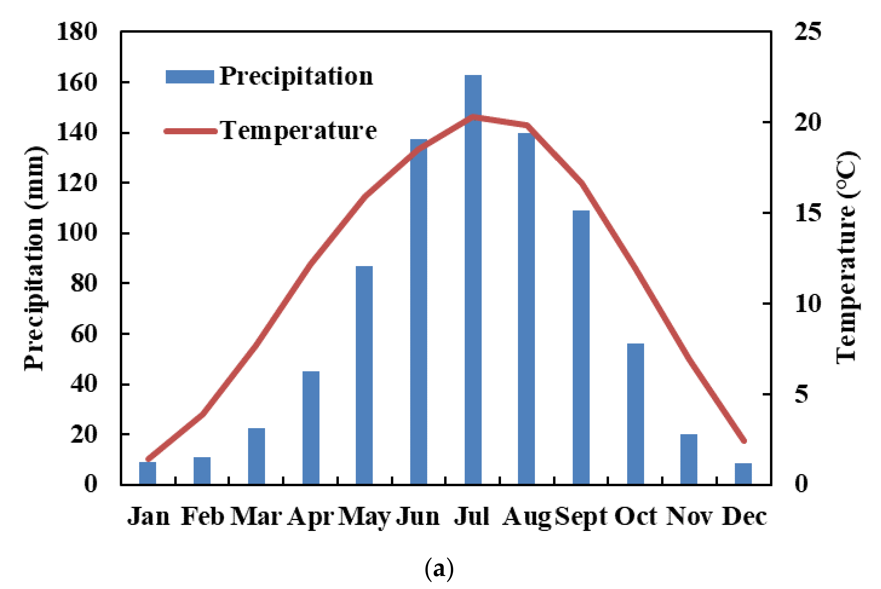
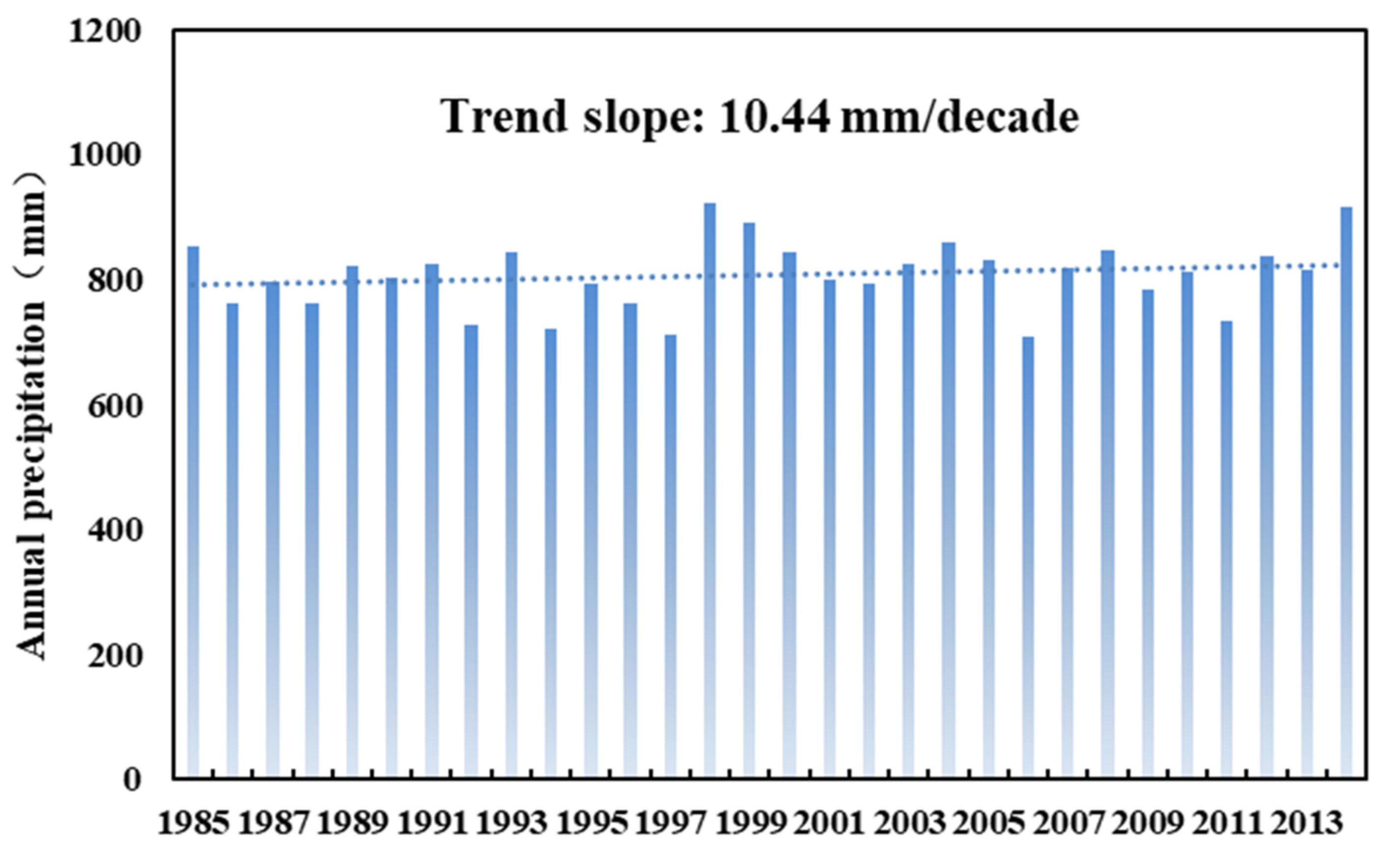
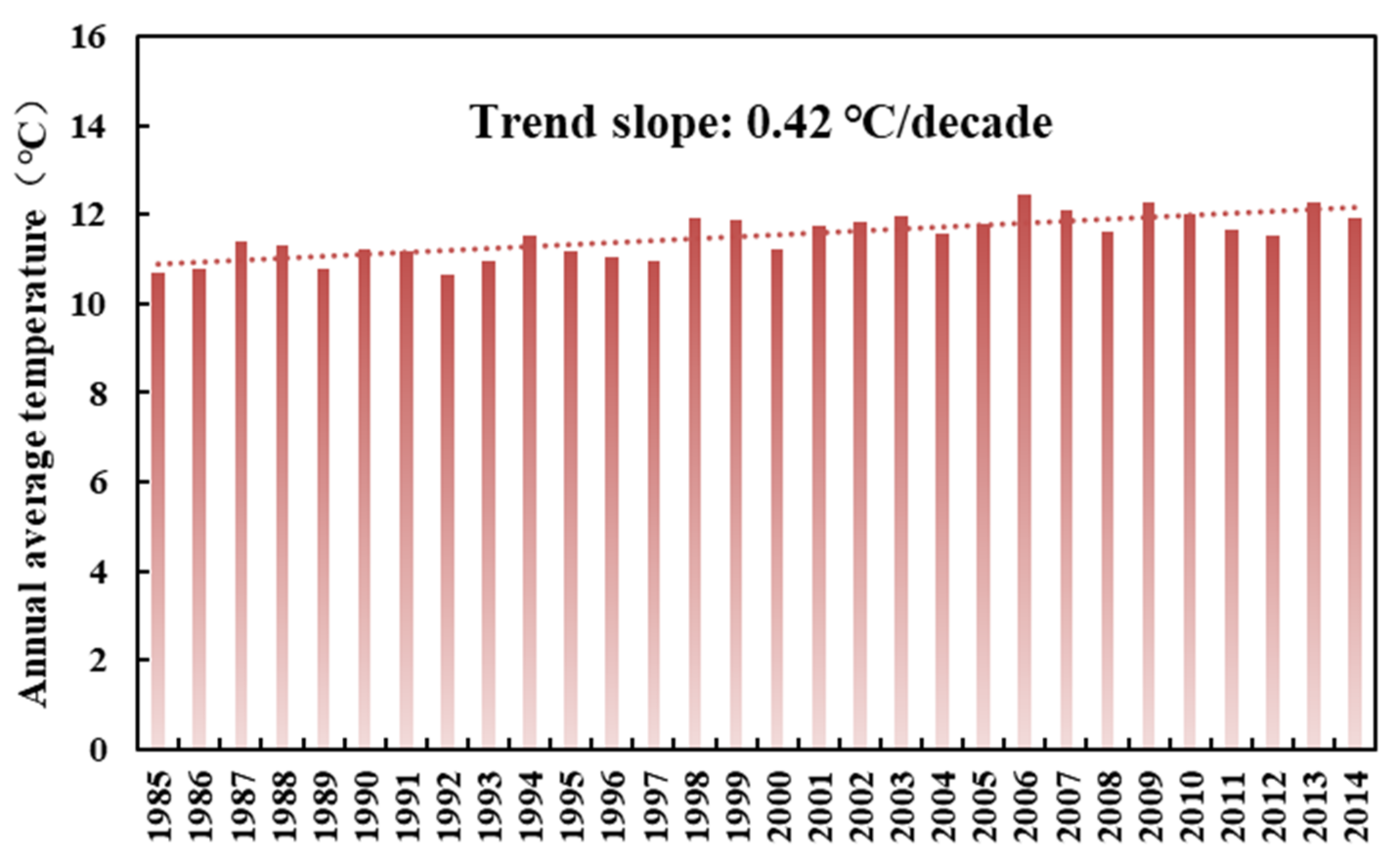
3.1.1. Temporal Variation Patterns of Precipitation and Temperature
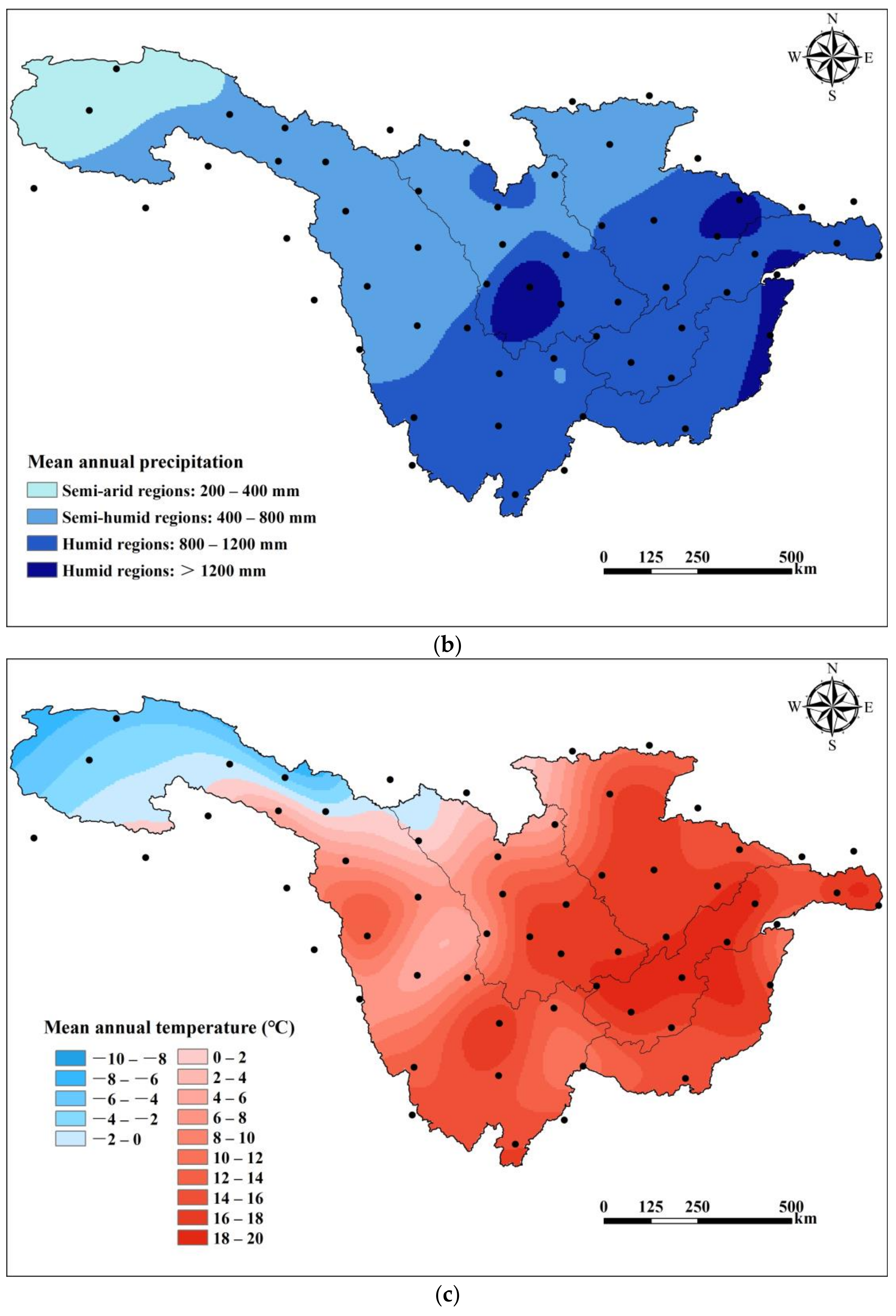
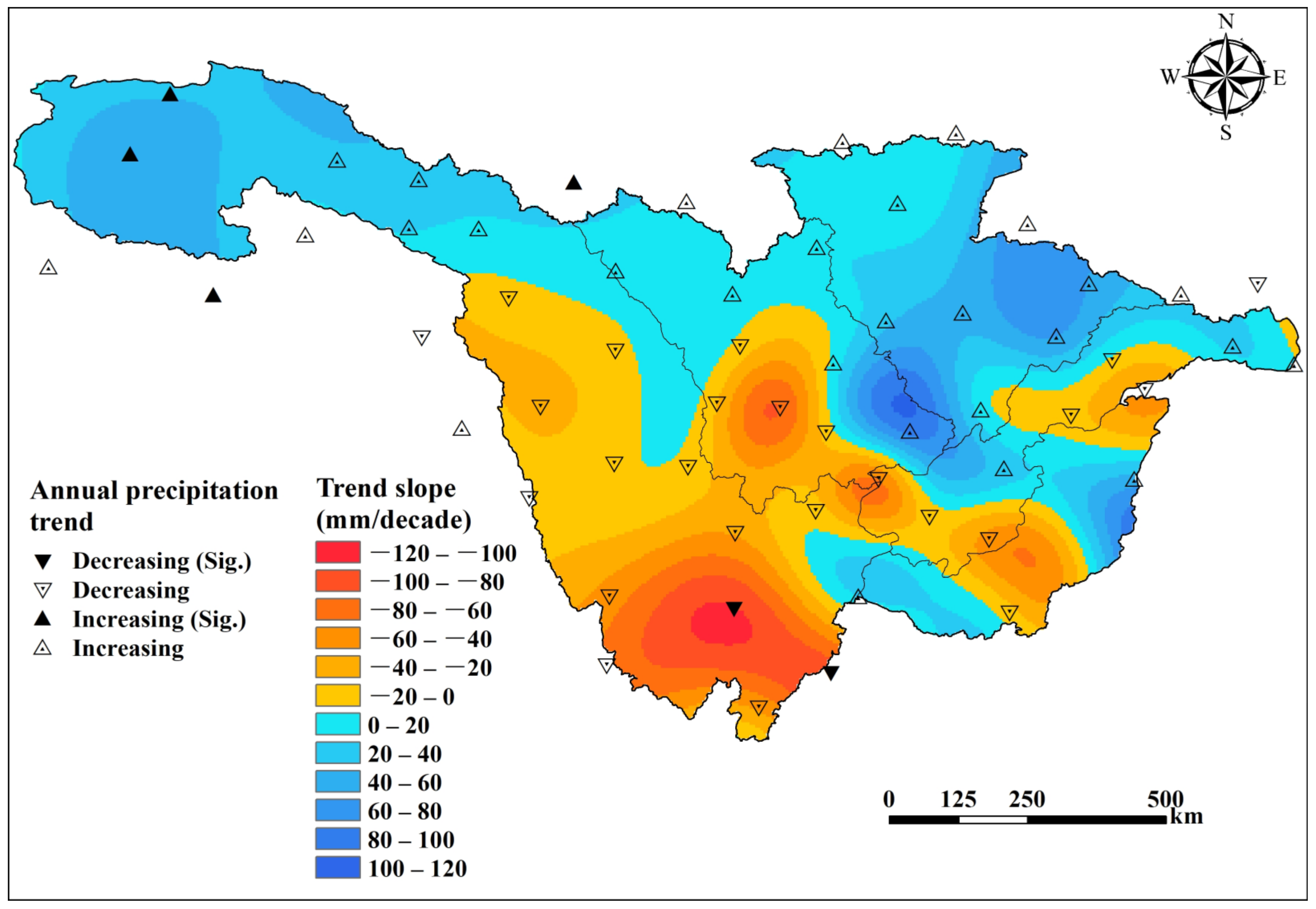
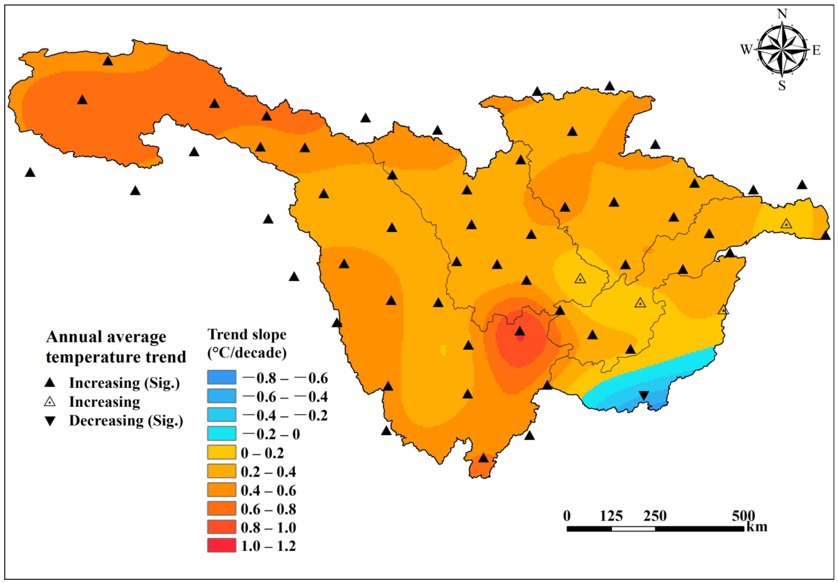
3.1.2. Spatial Variation Patterns of Precipitation and Temperature
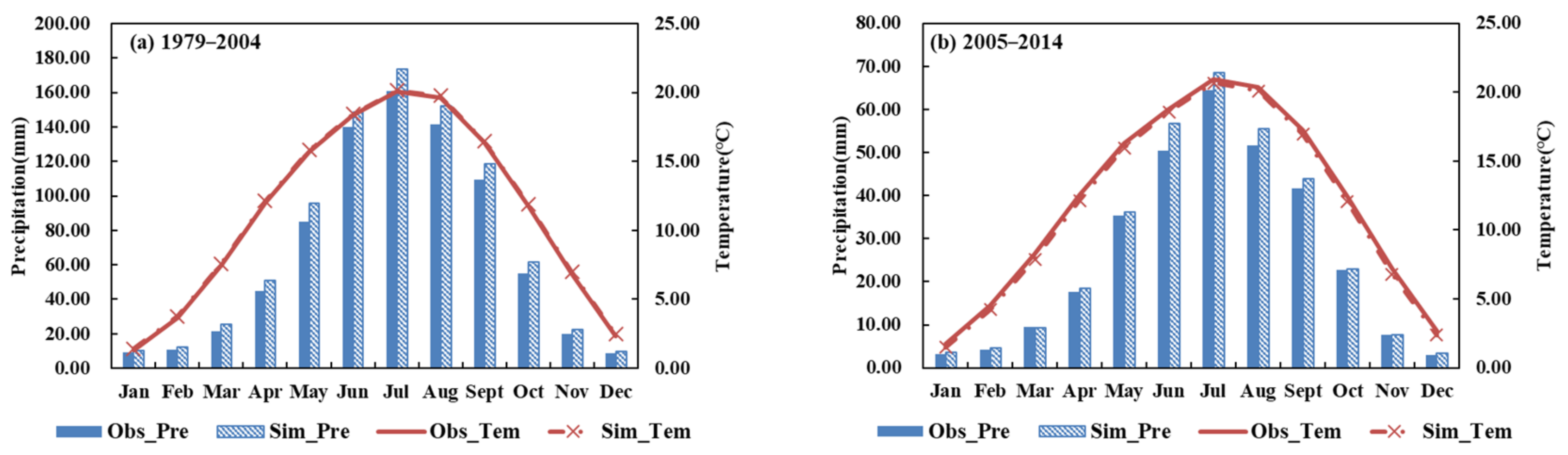
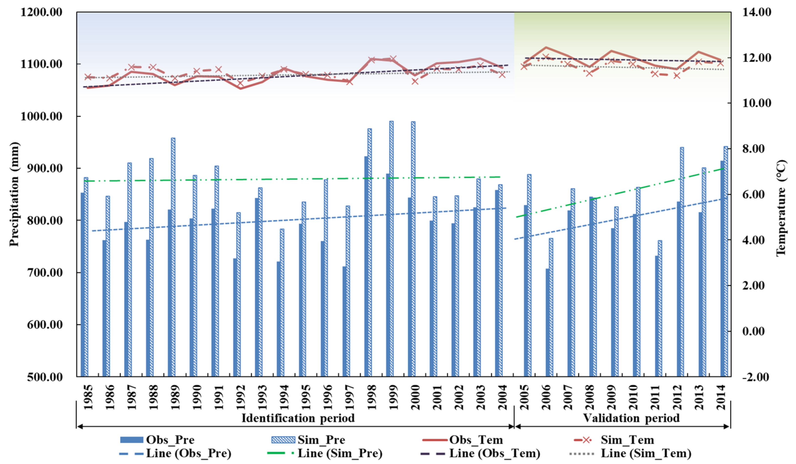
3.2. Identification and Verification of Statistical Downscaling Model
3.3. Future Climate Change in the Upper Yangtze River Basin
3.3.1. Temporal Variation Patterns of Future Precipitation and Temperature
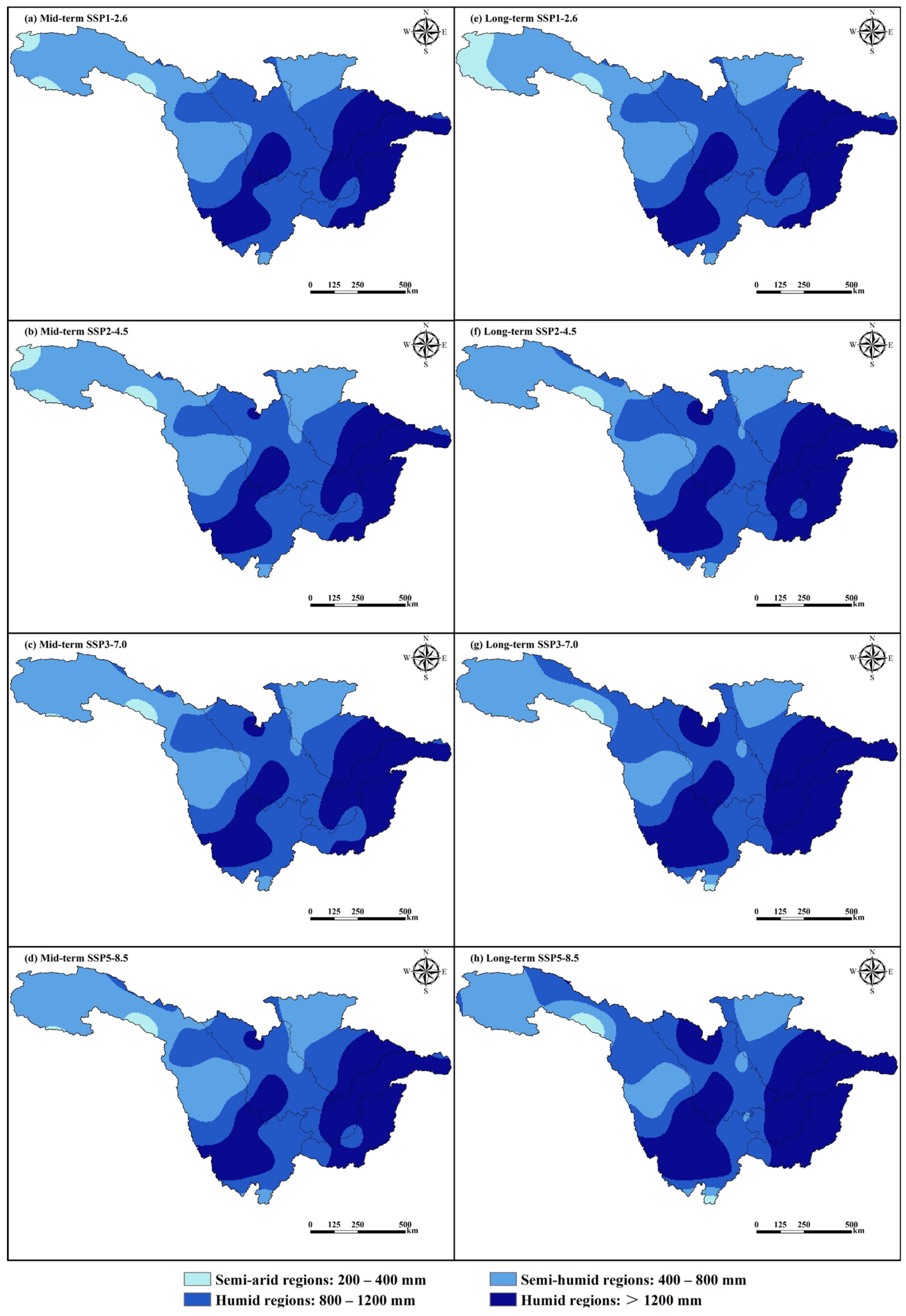
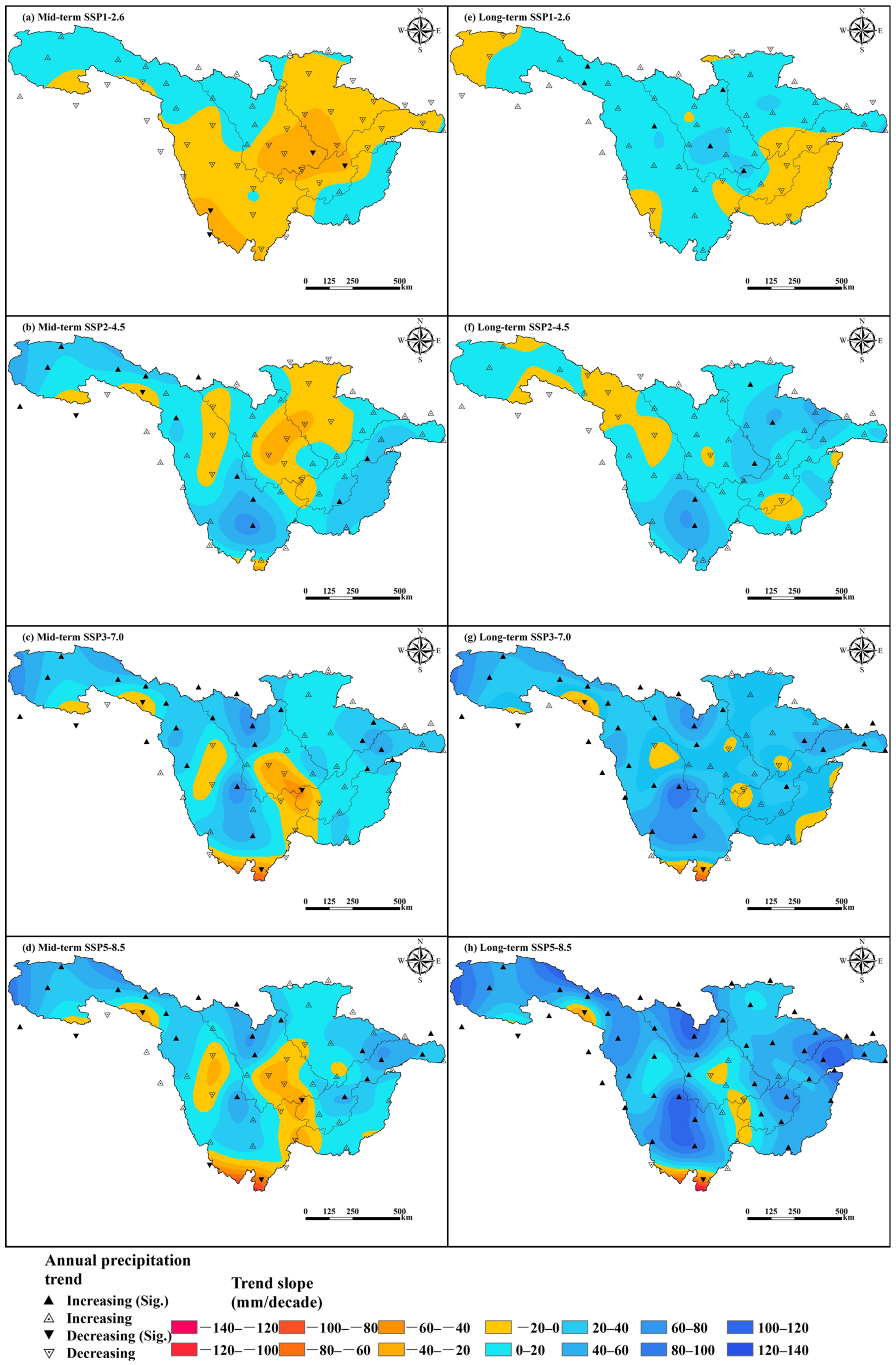
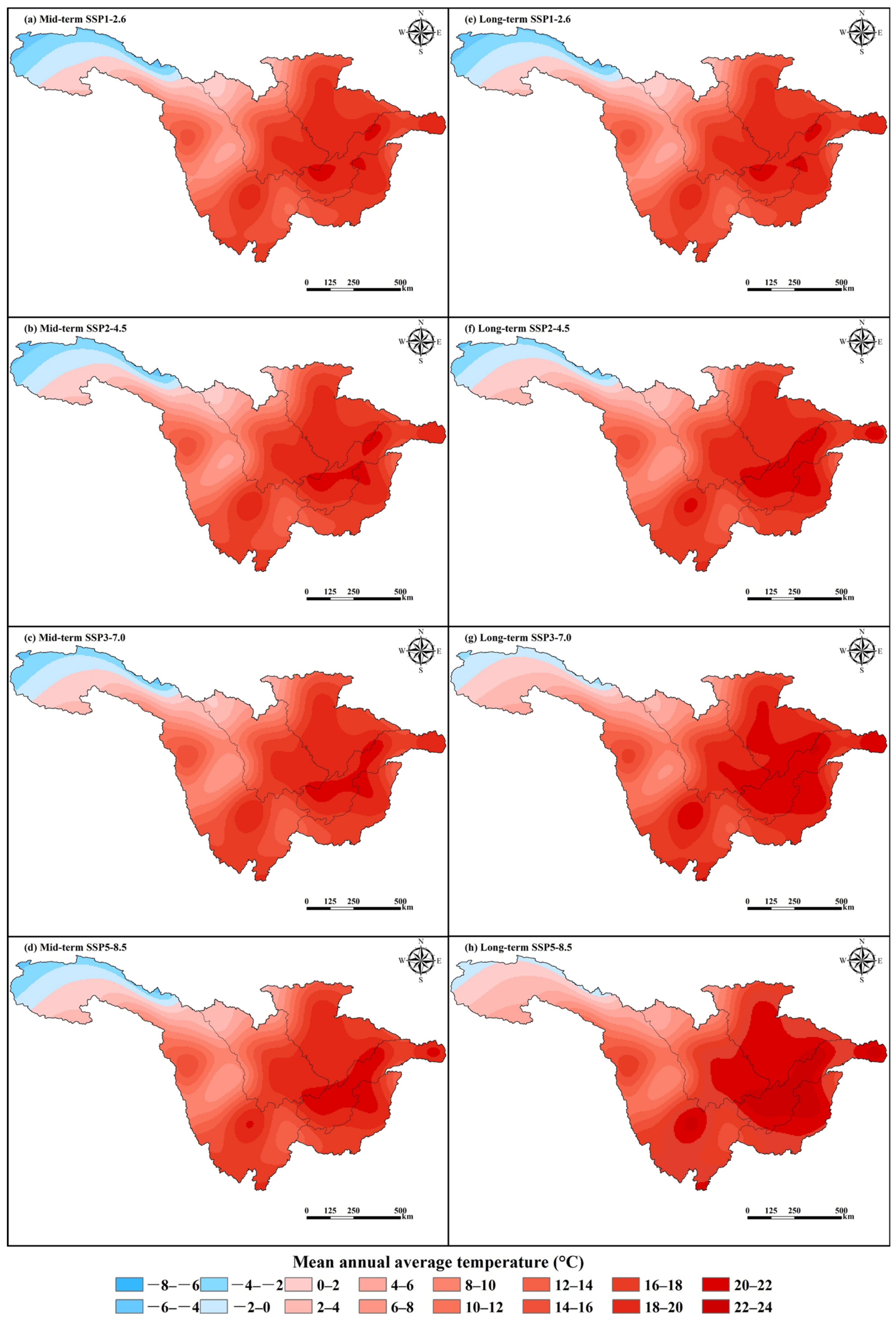
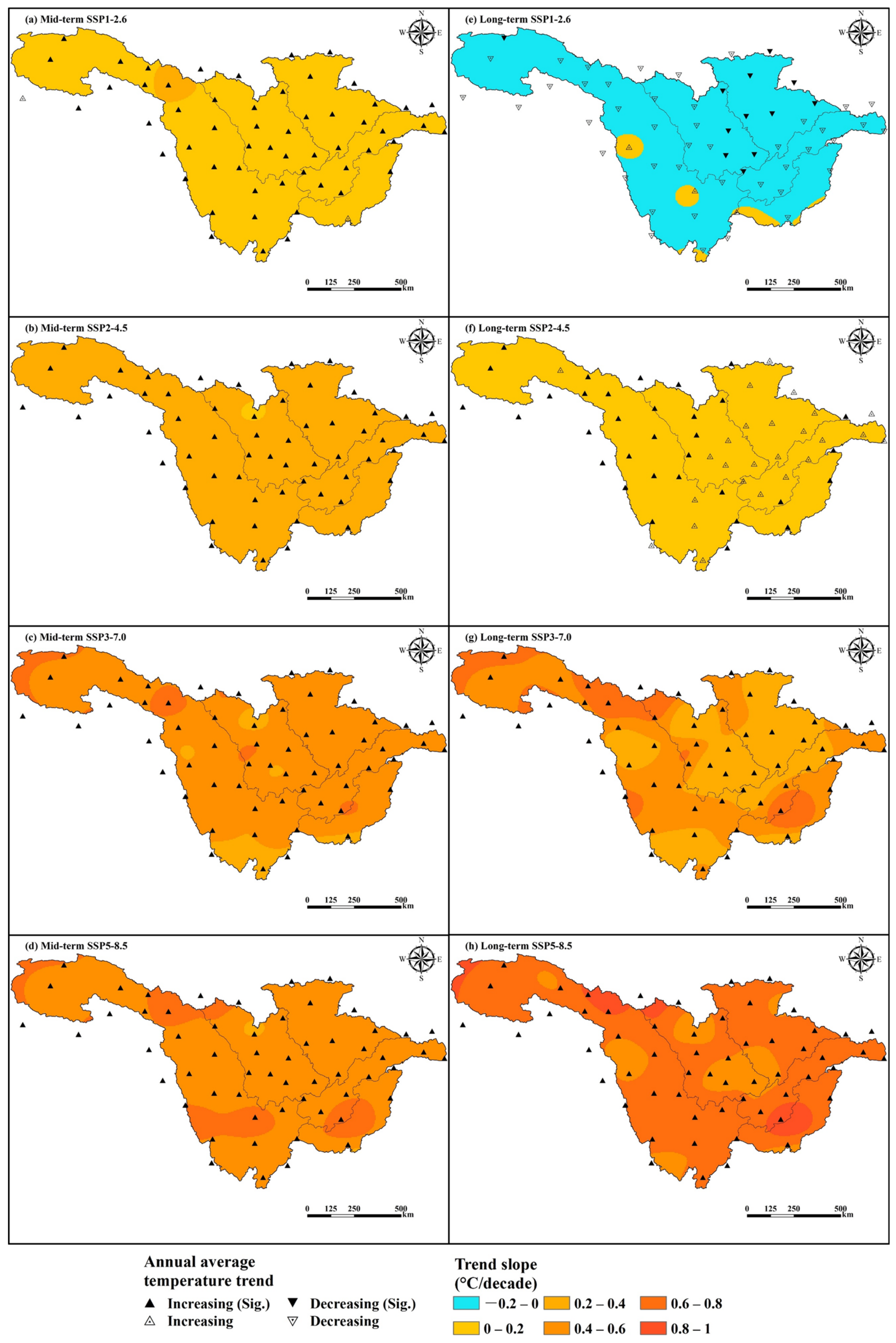
3.3.2. Spatial Variation Patterns of Future Precipitation and Temperature
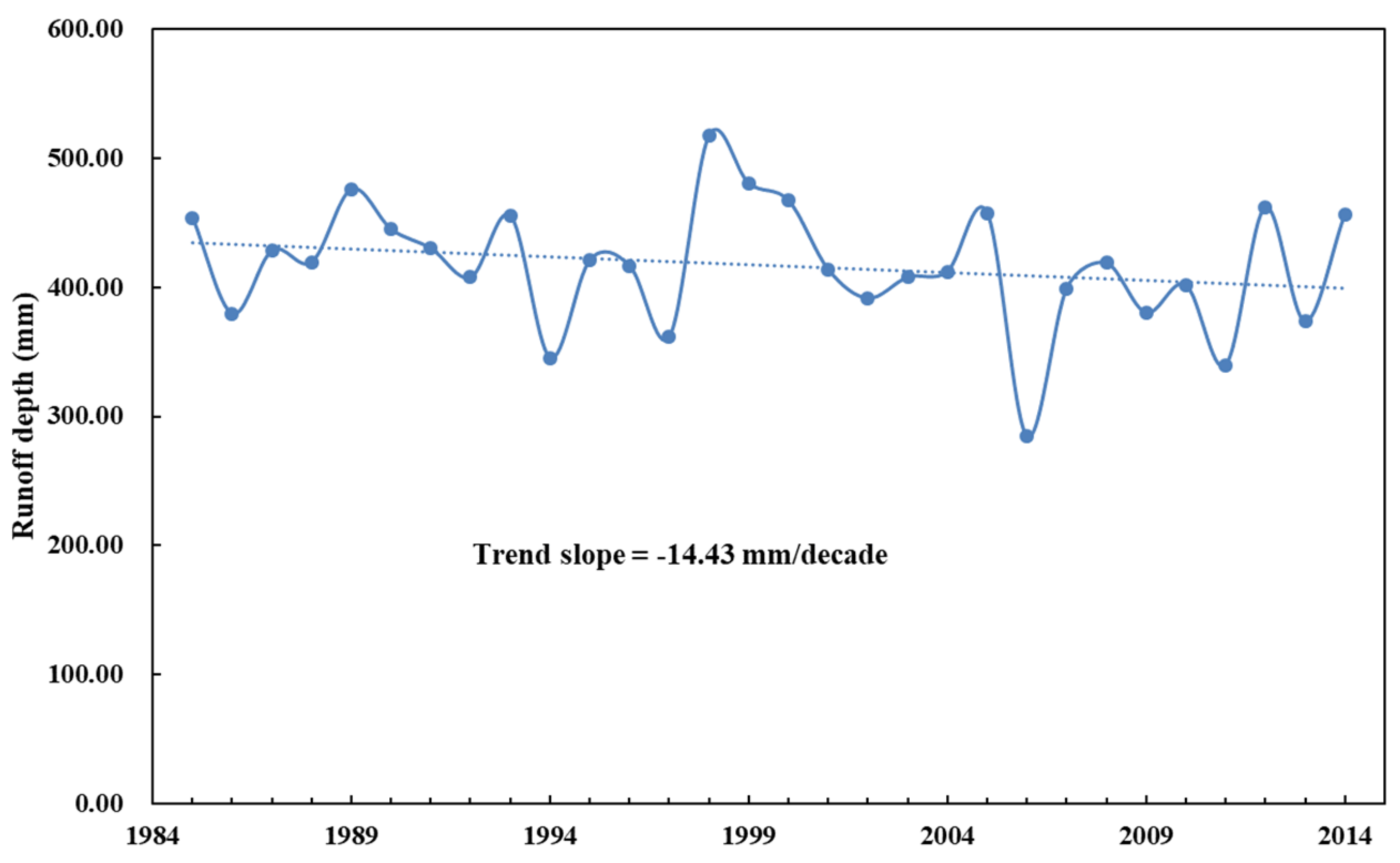
3.4. The Influence of Climate Change on Surface Runoff
3.4.1. Key Climatic Factors Affecting Surface Runoff
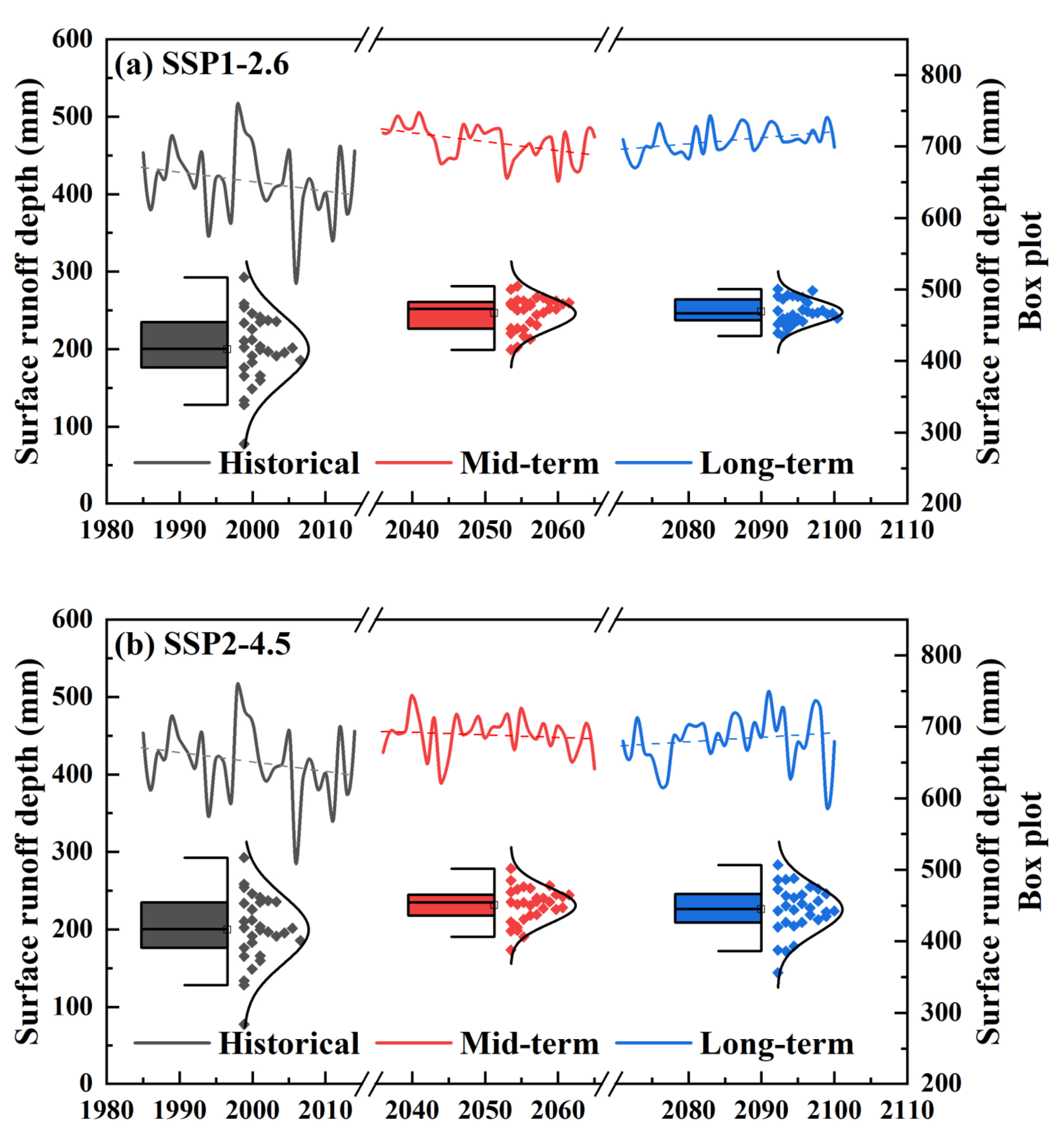
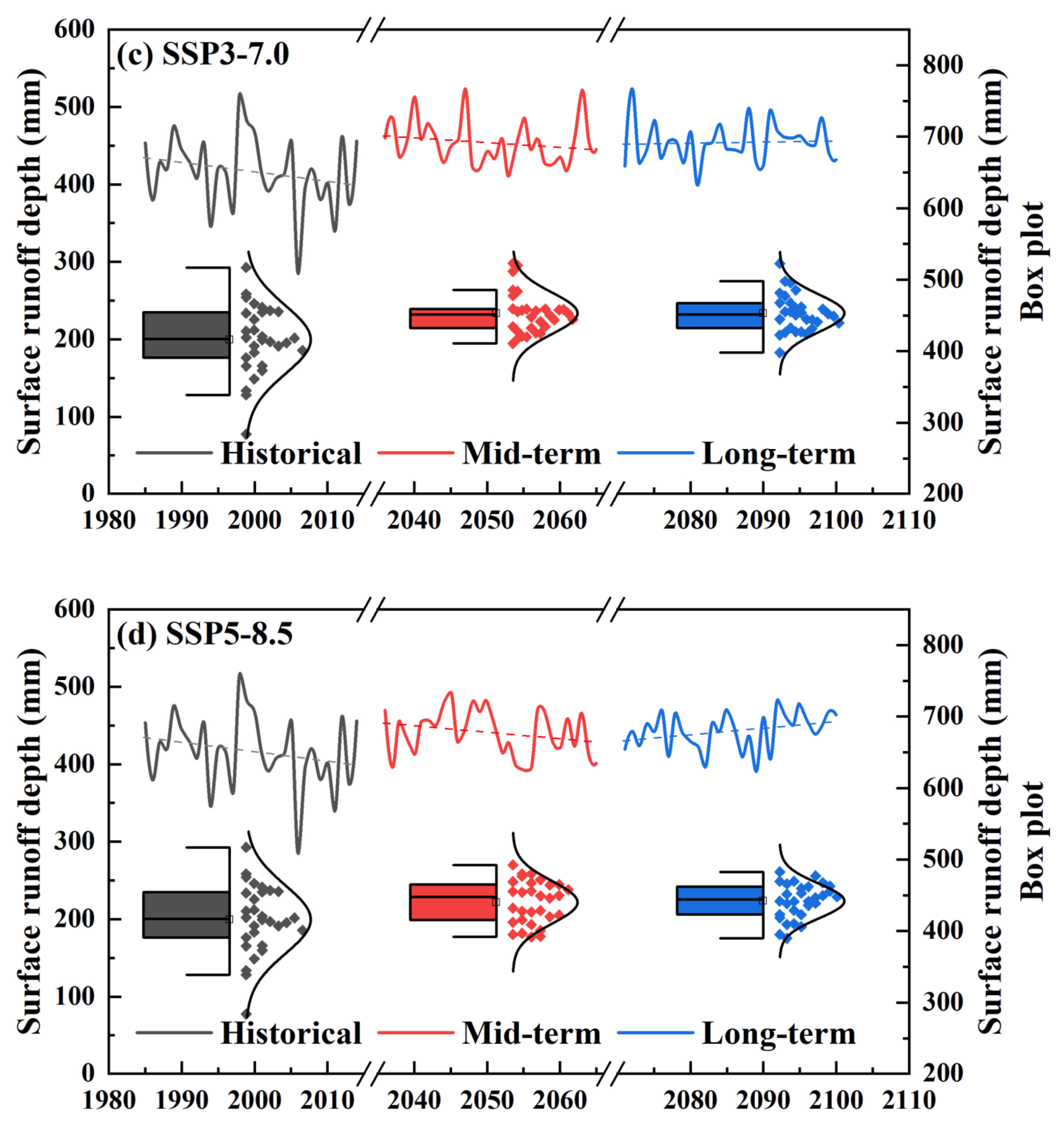
3.4.2. Changes in Future Surface Runoff
4. Discussion and Limitations of the Study
4.1. Discussion
4.2. Limitations of This Study
5. Conclusions
- (1)
- During the historical period (1985–2014), the UYRB experienced warming and humidification trends, with both annual precipitation and temperature increasing over time. The warming and humidification trends were more pronounced in the northwestern and central regions.
- (2)
- Under SSP1-2.6, SSP2-4.5, SSP3-7.0, and SSP5-8.5, relative to those in the historical period (1985–2014), the mean annual precipitation (MAP) and mean annual average temperature (MAT) over the UYRB increase in the future. The MAP and MAT values increase more in the long term (2071–2100) than in the mid-term (2036–2065).
- (3)
- Under SSP2-4.5, SSP3-7.0, and SSP5-8.5, precipitation and temperature show increasing trends in both the mid-term (2036–2065) and long term (2071–2100). Under SSP1-2.6, the precipitation series first decreases and then increases from the mid-term (2036–2065) to the long term (2071–2100), while the temperature first increases and then decreases. The trend slopes of precipitation and temperature are minimized under SSP1-2.6. This indicates that the sustainable development pathway is conducive to reducing the impact of climate change in the UYRB.
- (4)
- At the spatial scale, the humid regions (annual precipitation > 800 mm) and high-temperature regions (annual temperature > 20 °C) in the future are projected to increase. Conversely, the semi-arid regions (annual precipitation between 200 mm and 400 mm) and cold regions (annual temperature below 0 °C) are expected to decrease. These changes are enhanced with increasing values of radiative forcing. The slopes of precipitation and temperature are greater in high-altitude regions than those in low-altitude regions.
- (5)
- The introduction of the random forest regression algorithm can effectively improve the credibility of the identification of key climatic factors influencing surface runoff. Apart from annual precipitation and annual average temperature, the key climatic factors influencing surface runoff also include the extreme climate indicator, R×5day. Precipitation and R×5day are positively correlated with surface runoff, and temperature is negatively correlated with surface runoff.
- (6)
- Under SSP1-2.6, SSP2-4.5, SSP3-7.0, and SSP5-8.5, the mean annual surface runoff (MAR) values in the UYRB are greater than those in the historical period in both the mid-term (2036–2065) and the long term (2071–2100). Surface runoff tends to decrease in the mid-term (2036–2065) due to temperature increases and to increase in the long term (2071–2100) due to precipitation increases. Under SSP1-2.6, the surface runoff increases significantly (at a 5% level), which means the risk of flood disaster in the future in the UYRB may increase under the scenario of lower radiative forcing.
Funding
Data Availability Statement
Acknowledgments
Conflicts of Interest
Appendix A

| Number | Station Name | Short Name | Code | Latitude (°N) | Longitude (°E) |
|---|---|---|---|---|---|
| 1 | Wudaoliang | WDL | 52908 | 35.22 | 93.08 |
| 2 | Anduo | AND | 55294 | 32.35 | 91.10 |
| 3 | Tuotuohe | TTH | 56004 | 34.22 | 92.43 |
| 4 | Zaduo | ZAD | 56018 | 32.88 | 95.28 |
| 5 | Qumalai | QML | 56021 | 34.12 | 95.80 |
| 6 | Yushu | YUS | 56029 | 33.00 | 96.97 |
| 7 | Qingshuihe | QSH | 56034 | 33.80 | 97.13 |
| 8 | Shiqu | SHQ | 56038 | 32.98 | 98.10 |
| 9 | Dari | DAR | 56046 | 33.75 | 99.65 |
| 10 | Jiuzhi | JZH | 56067 | 33.43 | 101.48 |
| 11 | Minxian | MNX | 56093 | 34.43 | 104.02 |
| 12 | Wudu | WUD | 56096 | 33.40 | 104.92 |
| 13 | Suoxian | SUX | 56106 | 31.88 | 93.78 |
| 14 | Changdu | CHD | 56137 | 31.15 | 97.17 |
| 15 | Dege | DEG | 56144 | 31.80 | 98.58 |
| 16 | Seda | SED | 56152 | 32.28 | 100.33 |
| 17 | Ma’erkang | MEK | 56172 | 31.90 | 102.23 |
| 18 | Xiaojin | XAJ | 56178 | 31.00 | 102.35 |
| 19 | Songpan | SNP | 56182 | 32.67 | 103.60 |
| 20 | Wenjiang | WEJ | 56187 | 30.75 | 103.87 |
| 21 | Mianyang | MAY | 56196 | 31.45 | 104.73 |
| 22 | Batang | BAT | 56247 | 30.00 | 99.10 |
| 23 | Xinlong | XNL | 56251 | 30.93 | 100.32 |
| 24 | Ya’an | YAN | 56287 | 29.98 | 103.00 |
| 25 | Zuogong | ZUG | 56331 | 29.67 | 97.83 |
| 26 | Daocheng | DAC | 56357 | 29.05 | 100.30 |
| 27 | Kangding | KAN | 56374 | 30.05 | 101.97 |
| 28 | Leshan | LSH | 56386 | 29.57 | 103.75 |
| 29 | Deqin | DEQ | 56444 | 28.48 | 98.92 |
| 30 | Jiulong | JUL | 56462 | 29.00 | 101.50 |
| 31 | Leibo | LEB | 56485 | 28.27 | 103.58 |
| 32 | Yibin | YBN | 56492 | 28.80 | 104.60 |
| 33 | Xichang | XIC | 56571 | 27.90 | 102.27 |
| 34 | Lijiang | LIJ | 56651 | 26.85 | 100.22 |
| 35 | Huili | HUL | 56671 | 26.65 | 102.25 |
| 36 | Weining | WEN | 56691 | 26.87 | 104.28 |
| 37 | Dali | DAL | 56751 | 25.70 | 100.18 |
| 38 | Zhanyi | ZHY | 56786 | 25.58 | 103.83 |
| 39 | Maiji | MAJ | 57014 | 34.57 | 105.87 |
| 40 | Hanzhong | HAZ | 57127 | 33.07 | 107.03 |
| 41 | Wanyuan | WAY | 57237 | 32.07 | 108.03 |
| 42 | Fangxian | FAX | 57259 | 32.03 | 110.77 |
| 43 | Langzhong | LZH | 57306 | 31.58 | 105.98 |
| 44 | Daxian | DXN | 57328 | 31.20 | 107.50 |
| 45 | Zhenping | ZHP | 57343 | 31.90 | 109.53 |
| 46 | Badong | BAD | 57355 | 31.03 | 110.37 |
| 47 | Wanzhou | WAZ | 57432 | 30.77 | 108.40 |
| 48 | Lichuan | LCH | 57439 | 30.28 | 108.93 |
| 49 | Yichang | YIC | 57461 | 30.73 | 111.37 |
| 50 | Dongxingqu | DON | 57503 | 29.62 | 105.12 |
| 51 | Hechuan | HEC | 57512 | 29.97 | 106.27 |
| 52 | Fengdu | FED | 57523 | 29.85 | 107.73 |
| 53 | Xuyong | XYA | 57608 | 28.17 | 105.43 |
| 54 | Qijiang | QIJ | 57612 | 29.00 | 106.65 |
| 55 | Youyang | YOU | 57633 | 28.82 | 108.77 |
| 56 | Renhuai | REH | 57710 | 27.80 | 106.40 |
| 57 | Guiyang | GUI | 57816 | 26.58 | 106.73 |
| 58 | Kunming | KUN | 56778 | 25.00 | 102.65 |
| Station | Annual Mean Precipitation | Annual Mean Temperature | ||
|---|---|---|---|---|
| ZMK | Slope (mm/Decade) | ZMK | Slope (°C/Decade) | |
| AND | 1.36 | 21.79 | 4.14 * | 0.46 |
| SUX | 2.00 * | 43.77 | 3.82 * | 0.50 |
| TTH | 3.21 * | 53.45 | 4.57 * | 0.72 |
| WDL | 3.07 * | 38.58 | 4.17 * | 0.54 |
| YUS | 0.89 | 21.50 | 3.46 * | 0.50 |
| ZAD | 0.71 | 9.20 | 4.50 * | 0.58 |
| QML | 1.93 | 35.84 | 5.17 * | 0.70 |
| BAT | −1.00 | −25.89 | 3.75 * | 0.46 |
| DEQ | −0.11 | −7.29 | 4.03 * | 0.49 |
| ZUG | 0.16 | 1.50 | 3.75 * | 0.39 |
| CHD | −1.30 | −29.30 | 3.43 * | 0.35 |
| DEG | −0.29 | −7.40 | 3.28 * | 0.30 |
| SHQ | 0.87 | 16.27 | 3.71 * | 0.54 |
| DAR | 2.00 * | 36.36 | 4.28 * | 0.54 |
| QSH | 1.57 | 30.67 | 4.71 * | 0.66 |
| KUN | −0.68 | −42.82 | 4.03 * | 0.61 |
| DAL | −1.46 | −63.44 | 4.07 * | 0.45 |
| HUL | −2.43 * | −101.83 | 3.64 * | 0.38 |
| LIJ | −1.64 | −49.71 | 3.28 * | 0.43 |
| XIC | −0.75 | −38.62 | 3.25 * | 0.37 |
| DAC | −0.21 | −4.00 | 4.07 * | 0.45 |
| JUL | −0.29 | −6.59 | 3.14 * | 0.28 |
| KAN | −1.02 | −19.54 | 2.71 * | 0.29 |
| JZH | 0.70 | 16.28 | 4.25 * | 0.47 |
| MEK | 0.39 | 7.50 | 3.46 * | 0.35 |
| SED | 0.39 | 7.14 | 3.96 * | 0.38 |
| XAJ | −0.66 | −8.18 | 2.39 * | 0.30 |
| XNL | −0.07 | −4.44 | 3.32 * | 0.30 |
| WEN | 0.39 | 20.80 | 3.53 * | 0.44 |
| ZHY | −2.18 * | −90.75 | 3.71 * | 0.43 |
| DON | 0.68 | 87.94 | 0.32 | 0.06 |
| LSH | −0.46 | −13.18 | 3.18 * | 0.38 |
| LEB | −0.16 | −10.50 | 4.42 * | 0.99 |
| XYA | −0.32 | −11.78 | 2.85 * | 0.28 |
| YAN | −1.28 | −78.91 | 2.07 * | 0.23 |
| YBN | −1.25 | −60.67 | 3.75 * | 0.41 |
| MAY | 0.93 | 36.00 | 3.21 * | 0.47 |
| SNP | 1.14 | 17.36 | 3.14 * | 0.33 |
| WEJ | 0.04 | 6.54 | 2.96 * | 0.35 |
| WUD | 0.36 | 5.59 | 3.03 * | 0.37 |
| MNX | 0.54 | 12.07 | 3.96 * | 0.42 |
| GUI | −0.21 | −11.26 | −3.68 * | −0.42 |
| REH | −1.75 | −47.71 | 2.28 * | 0.20 |
| FED | −0.36 | −11.67 | 3.14 * | 0.35 |
| HEC | 0.21 | 11.60 | 3.10 * | 0.32 |
| QIJ | 0.75 | 29.88 | 0.86 | 0.11 |
| DXN | 1.28 | 61.00 | 3.21 * | 0.29 |
| HAZ | 1.50 | 73.56 | 5.10 * | 0.54 |
| LZH | 0.96 | 45.05 | 3.03 * | 0.32 |
| WAY | 1.28 | 59.00 | 2.50 * | 0.26 |
| MAJ | 0.57 | 14.53 | 3.14 * | 0.30 |
| LCH | −1.61 | −43.53 | 3.07 * | 0.29 |
| YOU | 0.71 | 48.20 | 1.89 | 0.21 |
| BAD | 0.61 | 22.79 | 1.21 | 0.11 |
| FAX | −0.29 | −4.92 | 2.32 * | 0.21 |
| WAZ | −0.18 | −4.75 | 3.57 * | 0.38 |
| ZHP | 0.64 | 27.67 | 2.60 * | 0.26 |
| YIC | 0.04 | 1.72 | 2.28 * | 0.29 |
| UYRB | 0.82 | 10.44 | 4.14 * | 0.42 |
| Station | Mid-Term (2036–2065) | Long-Term (2071–2100) | ||||||||||||||
|---|---|---|---|---|---|---|---|---|---|---|---|---|---|---|---|---|
| SSP1-2.6 | SSP2-4.5 | SSP3-7.0 | SSP5-8.5 | SSP1-2.6 | SSP2-4.5 | SSP3-7.0 | SSP5-8.5 | |||||||||
| ZMK | Slope | ZMK | Slope | ZMK | Slope | ZMK | Slope | ZMK | Slope | ZMK | Slope | ZMK | Slope | ZMK | Slope | |
| AND | 0.29 | 4.84 | 3.14 | 37.35 | 3.32 | 59.75 | 3.96 | 70.65 | −0.86 | −12.62 | 0.29 | 2.29 | 3.39 | 53.08 | 3.32 | 67.81 |
| SUX | −1.53 | −12.99 | −2.82 | −24.11 | −3.60 | −28.32 | −3.00 | −24.74 | 1.11 | 6.51 | −1.50 | −9.42 | −3.25 | −22.81 | −3.78 | −32.70 |
| TTH | 0.93 | 5.42 | 4.03 | 22.71 | 3.64 | 32.34 | 4.82 | 40.05 | −0.18 | −0.65 | 1.64 | 12.04 | 3.57 | 41.51 | 5.25 | 63.75 |
| WDL | 0.57 | 4.11 | 3.07 | 23.52 | 3.14 | 31.59 | 3.82 | 40.34 | −0.21 | −2.60 | 0.07 | 0.44 | 3.32 | 40.94 | 4.89 | 54.93 |
| YUS | −0.18 | −0.70 | −2.68 | −12.29 | −4.03 | −17.58 | −4.82 | −24.95 | 2.03 | 6.22 | 0.07 | 0.11 | −4.57 | −23.41 | −6.03 | −29.33 |
| ZAD | −0.89 | −5.15 | −0.29 | −2.54 | −0.32 | −3.80 | −0.11 | −1.04 | 0.54 | 2.32 | −1.21 | −10.75 | 1.07 | 9.37 | 2.96 | 24.82 |
| QML | 1.11 | 8.41 | 2.75 | 22.50 | 3.39 | 30.21 | 4.21 | 40.57 | 1.03 | 6.49 | 0.36 | 2.10 | 3.21 | 30.67 | 5.71 | 66.05 |
| BAT | −0.43 | −5.04 | 1.36 | 13.69 | 2.32 | 22.27 | 1.57 | 16.91 | 1.18 | 7.20 | 1.32 | 10.99 | 3.28 | 35.22 | 3.85 | 45.67 |
| DEQ | −1.25 | −10.67 | 1.64 | 15.31 | 0.46 | 7.32 | 1.68 | 12.38 | 0.61 | 6.67 | 1.39 | 17.50 | 2.75 | 29.92 | 3.21 | 39.17 |
| ZUG | −0.75 | −5.57 | 1.03 | 11.00 | 1.53 | 12.99 | 1.03 | 10.61 | 1.36 | 13.13 | 1.78 | 16.72 | 3.07 | 33.45 | 3.10 | 36.03 |
| CHD | −0.43 | −3.32 | 0.32 | 2.45 | 2.57 | 23.98 | 1.93 | 17.36 | 0.46 | 3.58 | −0.46 | −4.92 | 2.75 | 31.16 | 3.82 | 44.09 |
| DEG | 0.50 | 2.93 | 3.07 | 19.43 | 4.00 | 39.73 | 4.17 | 34.61 | 0.46 | 4.31 | −0.46 | −2.43 | 4.25 | 38.58 | 5.25 | 74.61 |
| SHQ | 0.75 | 4.67 | 1.61 | 10.56 | 2.32 | 19.23 | 1.96 | 17.68 | 1.11 | 7.22 | −0.93 | −7.91 | 2.82 | 23.58 | 4.89 | 54.08 |
| DAR | 1.50 | 10.52 | 2.32 | 19.46 | 2.96 | 21.85 | 3.64 | 36.62 | 1.89 | 13.95 | −0.11 | −1.61 | 3.35 | 33.61 | 5.03 | 62.98 |
| QSH | 1.21 | 8.56 | 2.46 | 21.41 | 2.85 | 22.50 | 3.28 | 31.43 | 2.03 | 13.79 | −0.43 | −2.11 | 3.60 | 34.30 | 5.14 | 61.20 |
| KUN | −1.18 | −17.59 | 0.04 | 1.04 | −2.11 | −45.93 | −3.18 | −62.66 | 0.54 | 9.27 | 1.82 | 27.93 | −2.11 | −37.41 | −2.53 | −60.56 |
| DAL | −2.25 | −34.73 | 0.46 | 4.73 | −1.21 | −26.09 | −2.57 | −47.59 | −0.18 | −3.72 | 0.00 | 0.00 | 0.71 | 9.56 | −0.64 | −18.50 |
| HUL | −0.39 | −5.44 | 2.71 | 65.10 | 1.96 | 41.76 | 1.14 | 27.39 | 1.18 | 18.76 | 2.36 | 58.17 | 3.50 | 68.20 | 3.78 | 95.88 |
| LIJ | −1.96 | −24.09 | 1.68 | 31.46 | 1.07 | 26.32 | 0.93 | 15.79 | −0.43 | −6.01 | 1.39 | 27.02 | 3.60 | 61.62 | 2.93 | 65.46 |
| XIC | 0.00 | −0.74 | 2.00 | 39.20 | 1.68 | 33.70 | 1.39 | 28.81 | 0.79 | 13.87 | 2.28 | 45.17 | 2.96 | 54.39 | 3.82 | 85.84 |
| DAC | −1.46 | −12.68 | −0.39 | −4.85 | −0.14 | −2.26 | −0.75 | −11.91 | 1.57 | 14.23 | 0.32 | 3.43 | 2.11 | 23.47 | 2.50 | 29.83 |
| JUL | −0.79 | −13.95 | 2.50 | 32.84 | 3.53 | 69.00 | 2.96 | 48.83 | 1.03 | 10.84 | 1.53 | 23.85 | 4.71 | 88.31 | 5.60 | 106.68 |
| KAN | 0.57 | 5.23 | 0.96 | 9.39 | 1.75 | 15.98 | 0.82 | 10.22 | 1.43 | 19.08 | 0.93 | 9.12 | 0.93 | 6.94 | 2.32 | 25.59 |
| JZH | 0.86 | 6.54 | 0.32 | 5.57 | 3.64 | 53.58 | 4.32 | 51.90 | 0.25 | 1.97 | 1.11 | 9.37 | 4.50 | 50.48 | 5.71 | 93.95 |
| MEK | 0.68 | 7.27 | 1.50 | 14.00 | 4.10 | 62.85 | 4.46 | 59.65 | 0.29 | 3.50 | 0.89 | 9.71 | 5.07 | 65.07 | 5.64 | 103.15 |
| SED | 0.25 | 1.91 | −1.07 | −8.45 | 2.28 | 24.56 | 1.93 | 14.62 | 1.64 | 11.11 | 0.25 | 3.84 | 2.75 | 27.62 | 4.50 | 52.85 |
| XAJ | 1.43 | 10.63 | 0.14 | 1.90 | 4.14 | 42.48 | 4.28 | 44.46 | 0.75 | 3.70 | 0.71 | 7.28 | 4.03 | 31.62 | 5.78 | 60.96 |
| XNL | −0.36 | −3.79 | −1.39 | −10.22 | −0.71 | −7.29 | −1.39 | −16.33 | 2.21 | 18.08 | −0.64 | −8.30 | −0.04 | −1.34 | 2.46 | 16.05 |
| WEN | −0.93 | −10.99 | 0.50 | 8.60 | −1.14 | −17.58 | −1.82 | −25.83 | 0.00 | −0.59 | 0.61 | 11.55 | 1.50 | 18.93 | 0.07 | 1.68 |
| ZHY | −0.46 | −3.72 | 1.39 | 24.90 | −0.25 | −3.93 | −0.07 | −1.74 | −0.07 | −0.10 | 0.93 | 18.34 | 1.75 | 33.48 | 1.71 | 30.29 |
| DON | −2.39 | −34.74 | 1.32 | 17.65 | 1.36 | 24.84 | 1.46 | 17.99 | 0.82 | 7.44 | 2.07 | 34.65 | 1.71 | 29.06 | 3.18 | 46.25 |
| LSH | −1.93 | −36.63 | −0.71 | −12.99 | −1.78 | −36.42 | −1.11 | −25.73 | 1.50 | 21.65 | 0.57 | 12.10 | 0.68 | 17.99 | 0.04 | 0.81 |
| LEB | −1.53 | −17.53 | 0.46 | 4.10 | −0.75 | −9.47 | −0.64 | −5.04 | −0.07 | −1.03 | 0.21 | 4.67 | 1.18 | 18.70 | 1.46 | 18.79 |
| XYA | −0.93 | −7.95 | 0.64 | 5.38 | −0.32 | −2.80 | 1.14 | 11.04 | 0.32 | 1.59 | 0.93 | 6.69 | 1.14 | 15.66 | 2.71 | 23.28 |
| YAN | −1.14 | −26.34 | −1.03 | −31.06 | −1.32 | −31.36 | −1.46 | −34.33 | 2.21 | 34.15 | −0.04 | −2.20 | 0.61 | 13.91 | −0.36 | −3.06 |
| YBN | −1.75 | −29.15 | −1.03 | −19.09 | −2.32 | −42.93 | −2.18 | −36.57 | 2.03 | 26.99 | 1.21 | 22.49 | −0.86 | −11.88 | −0.86 | −9.64 |
| MAY | −1.53 | −20.87 | −1.50 | −25.77 | 0.68 | 8.49 | −0.21 | −3.17 | 1.32 | 16.80 | 1.75 | 23.47 | 0.46 | 12.99 | 2.46 | 35.47 |
| SNP | −0.07 | −0.64 | 0.57 | 4.60 | 2.85 | 22.80 | 3.78 | 30.26 | 1.96 | 15.53 | 1.89 | 12.70 | 3.39 | 32.90 | 5.64 | 56.37 |
| WEJ | −0.96 | −18.09 | −1.89 | −28.12 | 0.50 | 7.37 | −1.14 | −18.89 | 1.78 | 19.24 | 1.39 | 17.40 | −0.11 | −1.31 | 0.29 | 3.31 |
| WUD | −1.36 | −10.61 | −1.25 | −7.56 | 1.32 | 8.79 | 1.32 | 6.56 | 1.32 | 12.06 | 2.07 | 14.37 | 0.71 | 8.65 | 2.68 | 18.19 |
| MNX | 0.25 | 1.12 | −0.39 | −4.70 | 1.46 | 21.27 | 1.39 | 10.93 | −0.25 | −3.33 | 1.93 | 17.49 | 1.61 | 16.46 | 3.78 | 40.58 |
| GUI | 1.21 | 13.21 | 1.46 | 22.30 | 1.21 | 19.08 | 0.93 | 13.41 | −0.68 | −7.39 | 0.36 | 5.79 | 0.61 | 8.19 | 2.57 | 48.60 |
| REH | 0.86 | 10.19 | 2.00 | 24.06 | 1.71 | 20.38 | 1.21 | 13.29 | −1.82 | −19.02 | −0.39 | −7.28 | 1.18 | 13.55 | 2.25 | 45.01 |
| FED | −0.36 | −3.49 | 2.46 | 23.59 | 3.00 | 19.47 | 2.21 | 24.49 | −0.46 | −5.40 | 1.28 | 17.43 | 1.46 | 18.88 | 3.07 | 38.67 |
| HEC | −1.28 | −25.06 | 0.21 | 2.88 | 0.29 | 5.26 | 0.18 | 0.95 | −1.00 | −13.67 | 0.61 | 11.82 | −0.18 | −3.88 | 1.75 | 43.06 |
| QIJ | −2.14 | −23.68 | 1.50 | 18.62 | 0.36 | 5.78 | 2.60 | 41.04 | −0.79 | −5.88 | 1.25 | 16.78 | 2.25 | 24.47 | 4.03 | 70.54 |
| DXN | −0.89 | −8.34 | 0.50 | 7.08 | 2.57 | 38.56 | 2.28 | 40.35 | 0.64 | 6.24 | 1.32 | 23.65 | 3.21 | 47.03 | 5.14 | 76.90 |
| HAZ | −0.68 | −8.65 | 0.07 | 2.25 | 1.50 | 20.49 | 0.93 | 20.73 | 0.71 | 10.52 | 1.61 | 27.82 | 1.03 | 20.94 | 2.14 | 34.38 |
| LZH | −1.07 | −17.83 | −0.39 | −6.81 | 1.14 | 18.12 | 1.32 | 20.96 | 1.50 | 18.50 | 2.14 | 41.28 | 1.28 | 36.48 | 2.28 | 42.70 |
| WAY | −0.75 | −15.93 | 0.11 | 3.58 | 2.00 | 34.60 | 1.64 | 37.31 | 0.93 | 14.31 | 1.82 | 46.71 | 1.00 | 22.58 | 2.64 | 61.00 |
| MAJ | 0.46 | 4.35 | −0.18 | −3.43 | 1.50 | 20.64 | 0.75 | 7.02 | 0.00 | −0.57 | 1.68 | 22.02 | 1.28 | 21.22 | 2.78 | 33.00 |
| LCH | −0.11 | −0.52 | 1.93 | 38.13 | 2.14 | 32.81 | 1.89 | 36.42 | −0.04 | −1.80 | 0.18 | 2.53 | 1.36 | 17.61 | 3.43 | 100.78 |
| YOU | 0.89 | 12.01 | 1.21 | 26.38 | 0.68 | 11.83 | 0.57 | 9.44 | −0.11 | −1.18 | 0.71 | 15.84 | 0.07 | 0.22 | 2.53 | 56.77 |
| BAD | −1.18 | −10.60 | 1.43 | 17.07 | 1.46 | 23.08 | 2.28 | 38.00 | 0.46 | 3.07 | 1.25 | 18.48 | 2.07 | 35.42 | 3.60 | 59.35 |
| FAX | −0.29 | −2.41 | 1.00 | 12.64 | 1.86 | 20.81 | 2.18 | 32.25 | −0.32 | −2.31 | 0.75 | 12.08 | 3.00 | 41.28 | 3.43 | 53.46 |
| WAZ | −1.03 | −10.31 | 1.64 | 28.23 | 2.21 | 44.90 | 2.93 | 59.33 | 0.18 | 1.51 | 1.53 | 28.08 | 3.18 | 50.70 | 4.57 | 99.84 |
| ZHP | −0.89 | −8.12 | 0.89 | 12.53 | 1.32 | 19.73 | 1.86 | 38.40 | 0.68 | 9.17 | 1.11 | 22.32 | 2.64 | 53.75 | 3.57 | 79.28 |
| YIC | 0.32 | 3.87 | 1.03 | 16.33 | 0.93 | 22.52 | 1.50 | 26.25 | 1.61 | 30.17 | 1.00 | 20.85 | 2.18 | 41.49 | 2.36 | 53.35 |
| UYRB | −0.89 | −5.30 | 1.61 | 12.08 | 2.18 | 17.06 | 1.93 | 12.37 | 1.14 | 7.08 | 2.00 | 16.68 | 3.43 | 29.17 | 4.67 | 47.93 |
| Station | Mid-Term (2036–2065) | Long-Term (2071–2100) | ||||||||||||||
|---|---|---|---|---|---|---|---|---|---|---|---|---|---|---|---|---|
| SSP1-2.6 | SSP2-4.5 | SSP3-7.0 | SSP5-8.5 | SSP1-2.6 | SSP2-4.5 | SSP3-7.0 | SSP5-8.5 | |||||||||
| ZMK | Slope | ZMK | Slope | ZMK | Slope | ZMK | Slope | ZMK | Slope | ZMK | Slope | ZMK | Slope | ZMK | Slope | |
| AND | 1.46 | 0.11 | 4.46 | 0.30 | 6.17 | 0.66 | 5.92 | 0.68 | −0.93 | −0.06 | 2.07 | 0.09 | 5.28 | 0.54 | 6.21 | 0.78 |
| SUX | 2.03 | 0.12 | 4.82 | 0.29 | 6.21 | 0.61 | 6.21 | 0.61 | −0.57 | −0.03 | 2.78 | 0.09 | 5.46 | 0.53 | 6.14 | 0.71 |
| TTH | 2.46 | 0.12 | 4.96 | 0.29 | 6.14 | 0.57 | 5.89 | 0.53 | −1.32 | −0.05 | 2.11 | 0.07 | 5.46 | 0.51 | 6.35 | 0.69 |
| WDL | 2.43 | 0.16 | 4.89 | 0.33 | 5.92 | 0.61 | 6.10 | 0.60 | −2.14 | −0.08 | 2.00 | 0.08 | 5.71 | 0.57 | 6.35 | 0.72 |
| YUS | 2.71 | 0.18 | 5.21 | 0.32 | 6.14 | 0.58 | 6.42 | 0.58 | −0.96 | −0.05 | 3.03 | 0.10 | 5.50 | 0.53 | 6.17 | 0.70 |
| ZAD | 2.93 | 0.21 | 5.39 | 0.33 | 5.89 | 0.60 | 6.39 | 0.60 | −1.21 | −0.06 | 2.89 | 0.11 | 5.46 | 0.58 | 6.10 | 0.72 |
| QML | 2.57 | 0.16 | 5.39 | 0.31 | 5.67 | 0.55 | 6.14 | 0.52 | −1.53 | −0.06 | 1.75 | 0.07 | 5.96 | 0.51 | 6.14 | 0.61 |
| BAT | 4.07 | 0.17 | 4.57 | 0.24 | 6.07 | 0.42 | 6.39 | 0.44 | 0.61 | 0.02 | 2.36 | 0.08 | 5.46 | 0.43 | 6.46 | 0.56 |
| DEQ | 3.35 | 0.17 | 5.14 | 0.28 | 6.28 | 0.58 | 6.53 | 0.61 | −1.32 | −0.06 | 4.17 | 0.14 | 6.10 | 0.56 | 6.60 | 0.73 |
| ZUG | 3.50 | 0.18 | 4.75 | 0.27 | 5.67 | 0.52 | 6.46 | 0.58 | −0.79 | −0.04 | 3.28 | 0.14 | 5.74 | 0.55 | 6.39 | 0.68 |
| CHD | 2.85 | 0.19 | 5.14 | 0.33 | 5.82 | 0.53 | 6.21 | 0.55 | −1.28 | −0.07 | 2.50 | 0.09 | 5.46 | 0.51 | 5.89 | 0.67 |
| DEG | 3.35 | 0.18 | 5.21 | 0.29 | 5.78 | 0.50 | 6.42 | 0.51 | −1.57 | −0.07 | 2.32 | 0.08 | 5.64 | 0.47 | 6.24 | 0.62 |
| SHQ | 3.18 | 0.23 | 5.28 | 0.35 | 5.99 | 0.66 | 6.46 | 0.70 | −0.96 | −0.06 | 3.35 | 0.14 | 5.53 | 0.64 | 6.46 | 0.82 |
| DAR | 3.57 | 0.17 | 5.39 | 0.31 | 5.92 | 0.52 | 6.42 | 0.58 | −1.25 | −0.04 | 2.25 | 0.08 | 6.07 | 0.57 | 6.35 | 0.79 |
| QSH | 3.89 | 0.18 | 5.25 | 0.32 | 5.85 | 0.55 | 6.21 | 0.60 | −1.39 | −0.04 | 2.07 | 0.09 | 6.21 | 0.60 | 6.39 | 0.84 |
| KUN | 3.10 | 0.15 | 4.35 | 0.32 | 4.39 | 0.34 | 6.03 | 0.57 | −0.11 | 0.00 | 1.25 | 0.08 | 5.32 | 0.46 | 6.28 | 0.66 |
| DAL | 4.00 | 0.15 | 4.60 | 0.23 | 5.10 | 0.33 | 6.46 | 0.48 | −0.89 | −0.03 | 1.25 | 0.05 | 5.71 | 0.38 | 6.57 | 0.55 |
| HUL | 3.82 | 0.16 | 4.64 | 0.27 | 5.17 | 0.41 | 6.49 | 0.56 | −0.36 | −0.02 | 1.46 | 0.06 | 5.60 | 0.43 | 6.49 | 0.65 |
| LIJ | 4.00 | 0.18 | 4.42 | 0.27 | 5.28 | 0.46 | 6.49 | 0.59 | −0.54 | −0.03 | 2.07 | 0.09 | 5.71 | 0.47 | 6.49 | 0.68 |
| XIC | 2.85 | 0.13 | 4.03 | 0.31 | 4.78 | 0.42 | 6.07 | 0.67 | 0.07 | 0.00 | 1.61 | 0.08 | 5.17 | 0.50 | 6.28 | 0.76 |
| DAC | 3.71 | 0.17 | 4.96 | 0.24 | 6.10 | 0.53 | 6.60 | 0.54 | −0.89 | −0.03 | 3.71 | 0.13 | 6.10 | 0.50 | 6.60 | 0.68 |
| JUL | 3.64 | 0.16 | 4.92 | 0.23 | 5.92 | 0.46 | 6.64 | 0.52 | −1.07 | −0.04 | 3.14 | 0.10 | 5.96 | 0.46 | 6.60 | 0.63 |
| KAN | 3.25 | 0.16 | 4.39 | 0.30 | 5.99 | 0.57 | 6.03 | 0.55 | −1.46 | −0.05 | 3.28 | 0.13 | 5.74 | 0.51 | 6.53 | 0.76 |
| JZH | 3.35 | 0.18 | 4.78 | 0.31 | 5.99 | 0.60 | 6.24 | 0.61 | −1.82 | −0.09 | 2.60 | 0.12 | 5.92 | 0.56 | 6.49 | 0.77 |
| MEK | 3.75 | 0.13 | 4.60 | 0.18 | 5.53 | 0.34 | 6.07 | 0.38 | −1.53 | −0.05 | 3.03 | 0.09 | 6.03 | 0.32 | 6.64 | 0.46 |
| SED | 3.53 | 0.19 | 4.78 | 0.28 | 5.74 | 0.54 | 6.53 | 0.58 | −1.43 | −0.04 | 3.25 | 0.10 | 6.24 | 0.55 | 6.46 | 0.76 |
| XAJ | 2.82 | 0.16 | 5.07 | 0.28 | 6.21 | 0.58 | 6.32 | 0.57 | −1.86 | −0.07 | 2.85 | 0.09 | 6.03 | 0.49 | 6.49 | 0.72 |
| XNL | 3.18 | 0.16 | 4.92 | 0.25 | 5.89 | 0.47 | 6.60 | 0.51 | −1.89 | −0.04 | 3.35 | 0.08 | 5.99 | 0.44 | 6.35 | 0.63 |
| WEN | 2.50 | 0.12 | 4.07 | 0.27 | 4.82 | 0.47 | 5.92 | 0.59 | 0.07 | 0.01 | 2.25 | 0.16 | 5.10 | 0.49 | 6.49 | 0.73 |
| ZHY | 2.46 | 0.13 | 4.17 | 0.25 | 4.78 | 0.35 | 5.85 | 0.53 | −0.39 | −0.03 | 2.00 | 0.11 | 5.10 | 0.42 | 6.39 | 0.63 |
| DON | 3.03 | 0.14 | 4.96 | 0.27 | 5.82 | 0.42 | 5.85 | 0.45 | −2.32 | −0.07 | 0.96 | 0.05 | 5.96 | 0.40 | 6.49 | 0.59 |
| LSH | 3.00 | 0.14 | 5.00 | 0.25 | 5.78 | 0.40 | 6.07 | 0.42 | −1.96 | −0.07 | 1.46 | 0.05 | 5.74 | 0.36 | 6.60 | 0.57 |
| LEB | 3.21 | 0.16 | 5.03 | 0.29 | 5.74 | 0.50 | 6.14 | 0.54 | −1.39 | −0.07 | 2.32 | 0.11 | 5.96 | 0.46 | 6.74 | 0.70 |
| XYA | 3.25 | 0.16 | 4.75 | 0.28 | 5.82 | 0.48 | 6.03 | 0.52 | −1.86 | −0.06 | 1.86 | 0.09 | 5.74 | 0.44 | 6.64 | 0.68 |
| YAN | 2.68 | 0.13 | 4.85 | 0.25 | 5.89 | 0.41 | 5.85 | 0.42 | −1.82 | −0.06 | 1.86 | 0.06 | 5.64 | 0.35 | 6.64 | 0.56 |
| YBN | 3.10 | 0.15 | 4.92 | 0.27 | 5.82 | 0.42 | 5.92 | 0.47 | −2.36 | −0.07 | 1.46 | 0.06 | 5.74 | 0.41 | 6.60 | 0.61 |
| MAY | 3.43 | 0.15 | 5.03 | 0.29 | 6.14 | 0.48 | 6.39 | 0.48 | −2.39 | −0.08 | 1.61 | 0.07 | 5.92 | 0.41 | 6.74 | 0.62 |
| SNP | 3.18 | 0.16 | 4.75 | 0.27 | 6.32 | 0.52 | 6.39 | 0.54 | −1.96 | −0.06 | 3.10 | 0.13 | 6.21 | 0.48 | 6.67 | 0.68 |
| WEJ | 3.28 | 0.15 | 4.89 | 0.27 | 6.28 | 0.47 | 6.35 | 0.48 | −2.32 | −0.07 | 1.64 | 0.08 | 5.89 | 0.41 | 6.78 | 0.60 |
| WUD | 3.28 | 0.17 | 4.92 | 0.29 | 5.89 | 0.47 | 6.17 | 0.51 | −2.03 | −0.08 | 0.79 | 0.05 | 5.78 | 0.43 | 6.53 | 0.64 |
| MNX | 3.14 | 0.16 | 5.00 | 0.27 | 6.21 | 0.52 | 6.46 | 0.52 | −1.75 | −0.04 | 2.28 | 0.08 | 5.89 | 0.46 | 6.64 | 0.66 |
| GUI | 1.64 | 0.07 | 4.46 | 0.26 | 5.10 | 0.37 | 5.78 | 0.49 | 0.00 | 0.00 | 2.07 | 0.16 | 5.46 | 0.42 | 6.14 | 0.62 |
| REH | 2.64 | 0.15 | 4.60 | 0.38 | 5.74 | 0.61 | 6.53 | 0.73 | −0.71 | −0.03 | 2.18 | 0.17 | 5.99 | 0.64 | 6.49 | 0.93 |
| FED | 3.14 | 0.14 | 4.85 | 0.27 | 5.85 | 0.45 | 5.96 | 0.51 | −1.07 | −0.04 | 1.82 | 0.09 | 5.89 | 0.44 | 6.57 | 0.65 |
| HEC | 3.35 | 0.14 | 4.53 | 0.25 | 5.74 | 0.42 | 5.85 | 0.46 | −0.54 | −0.02 | 1.32 | 0.06 | 5.74 | 0.40 | 6.17 | 0.59 |
| QIJ | 3.32 | 0.16 | 4.82 | 0.29 | 5.64 | 0.50 | 6.14 | 0.54 | −1.14 | −0.05 | 1.89 | 0.11 | 5.92 | 0.49 | 6.39 | 0.69 |
| DXN | 3.71 | 0.17 | 5.32 | 0.30 | 6.17 | 0.52 | 6.21 | 0.54 | −1.93 | −0.07 | 1.78 | 0.08 | 6.03 | 0.45 | 6.49 | 0.70 |
| HAZ | 3.57 | 0.17 | 4.82 | 0.27 | 5.85 | 0.43 | 5.92 | 0.46 | −2.18 | −0.07 | 0.11 | 0.01 | 5.60 | 0.37 | 6.21 | 0.60 |
| LZH | 3.57 | 0.16 | 5.03 | 0.27 | 5.96 | 0.46 | 6.10 | 0.49 | −2.57 | −0.07 | 1.14 | 0.04 | 5.60 | 0.39 | 6.42 | 0.62 |
| WAY | 3.32 | 0.16 | 5.00 | 0.27 | 5.92 | 0.49 | 6.14 | 0.53 | −2.21 | −0.07 | 1.39 | 0.07 | 5.78 | 0.43 | 6.46 | 0.68 |
| MAJ | 3.35 | 0.16 | 4.46 | 0.28 | 5.85 | 0.49 | 6.24 | 0.51 | −2.25 | −0.07 | 0.57 | 0.02 | 5.35 | 0.42 | 6.17 | 0.63 |
| LCH | 2.57 | 0.12 | 4.82 | 0.29 | 6.10 | 0.46 | 6.28 | 0.52 | −1.11 | −0.05 | 2.46 | 0.12 | 6.39 | 0.45 | 6.42 | 0.64 |
| YOU | 2.36 | 0.12 | 4.78 | 0.29 | 6.03 | 0.49 | 6.53 | 0.53 | −0.64 | −0.02 | 2.57 | 0.14 | 6.32 | 0.48 | 6.42 | 0.70 |
| BAD | 3.21 | 0.17 | 4.92 | 0.29 | 6.24 | 0.55 | 6.03 | 0.57 | −1.89 | −0.07 | 1.39 | 0.08 | 6.17 | 0.49 | 6.32 | 0.69 |
| FAX | 3.43 | 0.16 | 5.07 | 0.29 | 6.17 | 0.52 | 5.99 | 0.54 | −1.50 | −0.06 | 0.96 | 0.06 | 6.03 | 0.47 | 6.49 | 0.69 |
| WAZ | 3.43 | 0.15 | 5.28 | 0.27 | 6.24 | 0.47 | 6.42 | 0.49 | −1.89 | −0.05 | 1.82 | 0.07 | 6.46 | 0.43 | 6.60 | 0.62 |
| ZHP | 3.10 | 0.17 | 4.64 | 0.31 | 6.42 | 0.56 | 6.17 | 0.59 | −1.78 | −0.06 | 1.96 | 0.10 | 6.07 | 0.51 | 6.46 | 0.77 |
| YIC | 2.43 | 0.13 | 4.39 | 0.32 | 5.57 | 0.54 | 5.78 | 0.55 | −1.71 | −0.07 | 1.89 | 0.12 | 5.78 | 0.51 | 6.35 | 0.71 |
| UYRB | 3.71 | 0.16 | 5.39 | 0.29 | 6.07 | 0.47 | 6.60 | 0.54 | −1.75 | −0.05 | 2.82 | 0.10 | 6.53 | 0.45 | 6.64 | 0.67 |
References
- Yonaba, R.; Mounirou, L.A.; Tazen, F.; Koïta, M.; Biaou, A.C.; Zouré, C.O.; Queloz, P.; Karambiri, H.; Yacouba, H. Future climate or land use? Attribution of changes in surface runoff in a typical Sahelian landscape. Comptes Rendus. Géoscience 2023, 335, 1–28. [Google Scholar] [CrossRef]
- Li, Y.; Yan, D.; Peng, H.; Xiao, S. Evaluation of precipitation in CMIP6 over the Yangtze River Basin. Atmos. Res. 2021, 253, 105406. [Google Scholar] [CrossRef]
- Gou, J.J.; Miao, C.Y.; Duan, Q.Y.; Tang, Q.H.; Di, Z.H.; Liao, W.H.; Wu, J.W.; Zhou, R. Sensitivity Analysis-Based Automatic Parameter Calibration of the VIC Model for Streamflow Simulations Over China. Water Resour. Res. 2020, 56, e2019WR025968. [Google Scholar] [CrossRef]
- IPCC. Summary for policymakers. Global warming of 1.5 °C. In An IPCC Special Report on the Impacts of Global Warming of 1.5 °C above Pre-Industrial Levels and Related Global Greenhouse Gas Emission Pathways; World Meteorological Organization: Geneva, Switzerland, 2018; p. 32. [Google Scholar]
- Diffenbaugh, N.S.; Singh, D.; Mankin, J.S.; Horton, D.E.; Swain, D.L.; Touma, D.; Charland, A.; Liu, Y.J.; Haugen, M.; Tsiang, M.; et al. Quantifying the influence of global warming on unprecedented extreme climate events. Proc. Natl. Acad. Sci. USA 2017, 114, 4881–4886. [Google Scholar] [CrossRef] [PubMed]
- Trenberth, K.E.; Fasullo, J.T.; Shepherd, T.G. Attribution of climate extreme events. Nat. Clim. Change 2015, 5, 725–730. [Google Scholar] [CrossRef]
- Chen, J.; Gao, C.; Zeng, X.; Xiong, M.; Wang, Y.; Jing, C.; Krysanova, V.; Huang, J.; Zhao, N.; Su, B. Assessing changes of river discharge under global warming of 1.5 °C and 2 °C in the upper reaches of the Yangtze River Basin: Approach by using multiple- GCMs and hydrological models. Quat. Int. 2017, 453, 63–73. [Google Scholar] [CrossRef]
- Yang, R.; Xing, B. Spatio-Temporal Variability in Hydroclimate over the Upper Yangtze River Basin, China. Atmosphere 2022, 13, 317. [Google Scholar] [CrossRef]
- Seddon, A.W.R.; Macias-Fauria, M.; Long, P.R.; Benz, D.; Willis, K.J. Sensitivity of global terrestrial ecosystems to climate variability. Nature 2016, 531, 229–232. [Google Scholar] [CrossRef]
- Frame, D.J.; Rosier, S.M.; Noy, I.; Harrington, L.J.; Carey-Smith, T.; Sparrow, S.N.; Stone, D.A.; Dean, S.M. Climate change attribution and the economic costs of extreme weather events: A study on damages from extreme rainfall and drought. Clim. Change 2020, 162, 781–797. [Google Scholar] [CrossRef]
- Zhang, C.; Sun, F.; Sharma, S.; Zeng, P.; Mejia, A.; Lyu, Y.P.; Gao, J.; Zhou, R.; Che, Y. Projecting multi-attribute flood regime changes for the Yangtze River basin. J. Hydrol. 2023, 617, 128846. [Google Scholar] [CrossRef]
- Wu, L.; Wang, S.; Bai, X.; Chen, F.; Li, C.; Ran, C.; Zhang, S. Identifying the Multi-Scale Influences of Climate Factors on Runoff Changes in a Typical Karst Watershed Using Wavelet Analysis. Land 2022, 11, 1284. [Google Scholar] [CrossRef]
- Burns, D.A.; Klaus, J.; McHale, M.R. Recent climate trends and implications for water resources in the Catskill Mountain region, New York, USA. J. Hydrol. 2007, 336, 155–170. [Google Scholar] [CrossRef]
- Li, Z.; Xu, X.; Yu, B.; Xu, C.; Liu, M.; Wang, K. Quantifying the impacts of climate and human activities on water and sediment discharge in a karst region of southwest China. J. Hydrol. 2016, 542, 836–849. [Google Scholar] [CrossRef]
- Okafor, G.; Jimoh, O.D.; Larbi, K.I. Detecting Changes in Hydro-Climatic Variables during the Last Four Decades (1975–2014) on Downstream Kaduna River Catchment, Nigeria. Appl. Categ. Struct. 2017, 07, 161–175. [Google Scholar] [CrossRef]
- Wu, L.; Chen, D.; Yang, D.; Luo, G.; Wang, J.; Chen, F. Response of Runoff Change to Extreme Climate Evolution in a Typical Watershed of Karst Trough Valley, SW China. Atmosphere 2023, 14, 927. [Google Scholar] [CrossRef]
- Yang, Y.N.; Xu, C.C.; Yang, Y.H.; Hao, X.M.; Shen, Y.P. Hydrology and Water Resources Variation and Its Responses to Regional Climate Change in Xinjiang. Acta Geogr. Sin. 2009, 64, 1331–1341. [Google Scholar] [CrossRef]
- Labat, D.; Goddéris, Y.; Probst, J.L.; Guyot, J.L. Evidence for global runoff increase related to climate warming. Adv. Water Resour. 2004, 27, 631–642. [Google Scholar] [CrossRef]
- Qian, J.; Zhou, B.T. Changes of weather and climate extremes in the IPCC AR6. Adv. Clim. Change Res. 2021, 17, 713–718. [Google Scholar]
- IPCC. Climate Change 2021: The Physical Science Basis. 2021. Available online: https://www.ipcc.ch/report/ar6/wg1/downloads/report/IPCC_AR6_WGI_Full_Report.pdf (accessed on 15 June 2023).
- Min, R.; Gu, X.; Guan, Y.; Zhang, X. Increasing likelihood of global compound hot-dry extremes from temperature and runoff during the past 120 years. J. Hydrol. 2023, 621, 129553. [Google Scholar] [CrossRef]
- Gray, L.C.; Zhao, L.; Stillwell, A.S. Impacts of climate change on global total and urban runoff. J. Hydrol. 2023, 620, 129352. [Google Scholar] [CrossRef]
- Nayak, P.C.; Sudheer, K.P.; Jain, S.K. Rainfall-runoff modeling through hybrid intelligent system. Water Resour. Res. 2007, 43, W07415. [Google Scholar] [CrossRef]
- Wang, Y.; Guo, S.; Chen, H.; Zhou, Y. Comparative study of monthly inflow prediction methods for the Three Gorges Reservoir. Stoch. Environ. Res. Risk Assess. 2014, 28, 555–570. [Google Scholar] [CrossRef]
- Li, W.; Yang, M.; Liang, Z.; Zhu, Y.; Mao, W.; Shi, J.; Chen, Y.-x. Assessment for surface water quality in Lake Taihu Tiaoxi River Basin China based on support vector machine. Stoch. Environ. Res. Risk Assess. 2013, 27, 1861–1870. [Google Scholar] [CrossRef]
- Hao, Z.; Hao, F.; Singh, V.P.; Ouyang, W. Quantitative risk assessment of the effects of drought on extreme temperature in eastern China. J. Geophys. Res. Atmos. 2017, 122, 9050–9059. [Google Scholar] [CrossRef]
- Lan, Y.; Shen, Y.; Zhong, Y.J.; Wu, S.F.; Wang, G.Y. Sensitivity of the mountain runoff of Urumqi River to the climate changes. J. Arid Land Resour. Environ. 2010, 24, 50–55. [Google Scholar]
- Labat, D. Cross wavelet analyses of annual continental freshwater discharge and selected climate indices. J. Hydrol. 2010, 385, 269–278. [Google Scholar] [CrossRef]
- Dong, L.J.; Dong, X.H.; Zeng, Q.; Wei, C.; Yu, D.; Bo, H.J.; Guo, J. Long-term runoff change trend of Yalong River basin under future climate change scenarios. Adv. Clim. Change Res. 2019, 15, 596–606. [Google Scholar]
- Qin, P.; Xu, H.; Liu, M.; Liu, L.; Xiao, C.; Mallakpour, I.; Naeini, M.R.; Hsu, K.; Sorooshian, S. Projected impacts of climate change on major dams in the Upper Yangtze River Basin. Clim. Change 2022, 170, 8. [Google Scholar] [CrossRef]
- Manoutsoglou, E.; Lazos, I.; Steiakakis, E.; Vafeidis, A. The Geomorphological and Geological Structure of the Samaria Gorge, Crete, Greece—Geological Models Comprehensive Review and the Link with the Geomorphological Evolution. Appl. Sci. 2022, 12, 10670. [Google Scholar] [CrossRef]
- Lipar, M.; Ferk, M. Karst pocket valleys and their implications on Pliocene–Quaternary hydrology and climate: Examples from the Nullarbor Plain, southern Australia. Earth-Sci. Rev. 2015, 150, 1–13. [Google Scholar] [CrossRef]
- Maity, R.; Ramadas, M.; Govindaraju, R.S. Identification of hydrologic drought triggers from hydroclimatic predictor variables. Water Resour. Res. 2013, 49, 4476–4492. [Google Scholar] [CrossRef]
- De Sousa, L.F.; Ferraz, L.L.; Santos, C.A.S.; Rocha, F.A.; de Jesus, R.M. Assessment of hydrological trends and changes in hydroclimatic and land use parameters in a river basin in northeast Brazil. J. S. Am. Earth Sci. 2023, 128, 104464. [Google Scholar] [CrossRef]
- Duan, K.; Yao, T.; Wang, N.; Liu, H. Numerical simulation of Urumqi Glacier No. 1 in the eastern Tianshan, central Asia from 2005 to 2070. Chin. Sci. Bull. 2012, 57, 4505–4509. [Google Scholar] [CrossRef]
- Zhao, S.Q.; Lv, X.Y.; Wang, Z.Y.; Zhao, Z.W.; Li, Y.X. Application of Machine Learning Techniques in Agrometeorology. Mod. Agric. Res. 2023, 29, 136–139. [Google Scholar] [CrossRef]
- Sun, J.L.; Zhang, Z.H.; Yu, W.D.; Deng, T.H. Research Progress on the Agrometeorological Automatic Observation in China. Adv. Meteorol. Sci. Technol. 2022, 12, 7–13+29. [Google Scholar] [CrossRef]
- Zuo, G.G. Study on Mechanism and Methods of Adaptive Streamflow Forecasting Based on Machine Learning. Ph.D. Thesis, Xi’an University of Technology, Xi’an, China, 2021. [Google Scholar]
- Wang, X.Y. Comparative Study on Agricultural Drought Monitoring in the Loess Plateau Based on Three Machine Learning Methods. Master’s Thesis, Northwest Normal University, Lanzhou, China, 2022. [Google Scholar]
- Xu, X.J. Estimation of Reference Evapotranspiration with Machine Learning Methods under Future Climate Change. Master’s Thesis, Northwest A&F University, Yangling, China, 2022. [Google Scholar]
- Li, X.; Zhang, L.; Zeng, S.; Tang, Z.; Liu, L.; Zhang, Q.; Tang, Z.; Hua, X. Predicting Monthly Runoff of the Upper Yangtze River Based on Multiple Machine Learning Models. Sustainability 2022, 14, 11149. [Google Scholar] [CrossRef]
- Wang, S.; Sun, M.; Wang, G.; Yao, X.; Wang, M.; Li, J.; Duan, H.; Xie, Z.; Fan, R.; Yang, Y. Simulation and Reconstruction of Runoff in the High-Cold Mountains Area Based on Multiple Machine Learning Models. Water 2023, 15, 3222. [Google Scholar] [CrossRef]
- Zhu, X.; Lee, S.-Y.; Wen, X.; Ji, Z.; Lin, L.; Wei, Z.; Zheng, Z.; Xu, D.; Dong, W. Extreme climate changes over three major river basins in China as seen in CMIP5 and CMIP6. Clim. Dyn. 2021, 57, 1187–1205. [Google Scholar] [CrossRef]
- Li, X.; Zhang, K.; Gu, P.; Feng, H.; Yin, Y.; Chen, W.; Cheng, B. Changes in precipitation extremes in the Yangtze River Basin during 1960–2019 and the association with global warming, ENSO, and local effects. Sci. Total Environ. 2021, 760, 144244. [Google Scholar] [CrossRef]
- Pang, Y.M.; Chen, C.; Xu, F.X.; Guo, X.Y. Impact of climate change on potential productivities of main grain crops in the Sichuan Basin. Chin. J. Ecol.-Agric. 2020, 28, 1661–1672. [Google Scholar] [CrossRef]
- Li, B.Y. Impact of Climate Change and Human Activities on Hydrological Processes in Upper Reaches of the Yangtze River Basin. Ph.D. Thesis, Wuhan University, Wuhan, China, 2020. [Google Scholar]
- National Oceanic and Atmospheric Administration, Physical Sciences Laboratory. NCEP-DOE Reanalysis 2: Summary. Available online: https://psl.noaa.gov/data/gridded/data.ncep.reanalysis2.html (accessed on 15 June 2023).
- World Meteorological Organization. No. 997—Scientists Urge More Frequent Updates of 30-Year Climate Baselines to Keep Pace with Rapid Climate Change. 6 December 2015. Available online: https://public.wmo.int/en/media/press-release/no-997-scientists-urge-more-frequent-updates-of-30-year-climate-baselines-keep (accessed on 15 June 2023).
- World Meteorological Organization. WMO Guidelines on the Calculation of Climate Normals; WMO: Geneva, Switzerland, 2017. Available online: https://library.wmo.int/index.php?lvl=notice_display&id=20130#.Xznu2ChKg2x (accessed on 15 June 2023).
- An, Y.K. Coupling Simulation and Uncertainty Analysis of Surface Water and Groundwater in Hun River Basin. Ph.D. Thesis, Jilin University, Changchun, China, 2019. [Google Scholar]
- Chen, J.; Brissette, F.P.; Leconte, R. Uncertainty of downscaling method in quantifying the impact of climate change on hydrology. J. Hydrol. 2011, 401, 190–202. [Google Scholar] [CrossRef]
- Wan, H.; Bian, J.; Zhang, H.; Li, Y. Assessment of future climate change impacts on water-heat-salt migration in unsaturated frozen soil using CoupModel. Front. Environ. Sci. Eng. 2020, 15, 10. [Google Scholar] [CrossRef]
- Gilbert, R.O. Statistical Methods for Environmental Pollution Monitoring; Wiley: Hoboken, NJ, USA, 1987. [Google Scholar]
- Wilby, R.L.; Dawson, C.W.; Barrow, E.M. sdsm—A decision support tool for the assessment of regional climate change impacts. Environ. Model. Softw. 2002, 17, 145–157. [Google Scholar] [CrossRef]
- Wilby, R.L.; Dawson, C.W. The Statistical DownScaling Model: Insights from one decade of application. Int. J. Climatol. 2013, 33, 1707–1719. [Google Scholar] [CrossRef]
- Hamed, K.H.; Ramachandra Rao, A. A modified Mann-Kendall trend test for autocorrelated data. J. Hydrol. 1998, 204, 182–196. [Google Scholar] [CrossRef]
- Mann, H.B. Nonparametric test against trend. Econometrica 1945, 13, 245–259. [Google Scholar] [CrossRef]
- Kendall, M.G. Rank Correlation Methods; Griffin: London, UK, 1948. [Google Scholar]
- Xianghui, L.U.; Hua, B.; Ya, L.V.; Benjia, Z. Analysis on Historical Weather and Prediction of Future Climate Change in Jiangxi Province. Res. Soil Water Conserv. 2015. [Google Scholar]
- Yonaba, R.; Tazen, F.; Cissé, M.; Mounirou, L.A.; Belemtougri, A.; Ouedraogo, V.A.; Koïta, M.; Niang, D.; Karambiri, H.; Yacouba, H. Trends, sensitivity and estimation of daily reference evapotranspiration ET0 using limited climate data: Regional focus on Burkina Faso in the West African Sahel. Theor. Appl. Climatol. 2023, 153, 947–974. [Google Scholar] [CrossRef]
- Yue, S.; Wang, C.Y. Applicability of prewhitening to eliminate the influence of serial correlation on the Mann-Kendall test. Water Resour. Res. 2002, 38, 4-1–4-7. [Google Scholar] [CrossRef]
- Asarian, J.E.; Walker, J.D. Long-Term Trends in Streamflow and Precipitation in Northwest California and Southwest Oregon, 1953-2012. JAWRA J. Am. Water Resour. Assoc. 2016, 52, 241–261. [Google Scholar] [CrossRef]
- Shourov, M.M.; Mahmud, I. pyMannKendall: A python package for non parametric Mann Kendall family of trend tests. J. Open Source Softw. 2019, 4, 1556. [Google Scholar] [CrossRef]
- Xiao, S.M.; Liu, T. Medium-term and long-term Forecast of Reservoir Runoff in Dry Season Based on Random Forest and Deep Neural Network. Guangdong Water Resour. Hydropower 2023, 54–58. [Google Scholar]
- Wang, Y.X.; Liu, X.; Shen, Y.J. Applicability of the random forest model in quantifying the attribution of runoff changes. Chin. J. Eco-Agric. 2022, 30, 864–874. [Google Scholar] [CrossRef]
- Thompson, C.G.; Kim, R.S.; Aloe, A.M.; Becker, B.J. Extracting the Variance Inflation Factor and Other Multicollinearity Diagnostics from Typical Regression Results. Basic Appl. Soc. Psychol. 2017, 39, 81–90. [Google Scholar] [CrossRef]
- Salmerón Gómez, R.; García Pérez, J.; López Martín, M.D.M.; García, C.G. Collinearity diagnostic applied in ridge estimation through the variance inflation factor. J. Appl. Stat. 2016, 43, 1831–1849. [Google Scholar] [CrossRef]
- Singh, A.K.; Kumar, P.; Ali, R.; Al-Ansari, N.; Vishwakarma, D.K.; Kushwaha, K.S.; Panda, K.C.; Sagar, A.; Mirzania, E.; Elbeltagi, A.; et al. An Integrated Statistical-Machine Learning Approach for Runoff Prediction. Sustainability 2022, 14, 8209. [Google Scholar] [CrossRef]
- Sharifi, A.; Dinpashoh, Y.; Mirabbasi, R. Daily runoff prediction using the linear and non-linear models. Water Sci. Technol. 2017, 76, 793–805. [Google Scholar] [CrossRef]
- Xie, S.; Zhang, K.; Li, Y.; Dai, C. Establishment of Low Water Runoff Forecast Model in Yichun River Basin by Multiple Linear Regression Method. IOP Conf. Ser. Earth Environ. Sci. 2020, 474, 072067. [Google Scholar] [CrossRef]
- Guo, C.W. Application of Combined Multiple Linear Regression Model in Runoff Prediction. Pearl River 2021, 42, 49–55. [Google Scholar] [CrossRef]
- Li, Y.J.; Li, X.; Tian, C.S. Application of Multiple Regression Method in Dry Season Runoff Forecast of Yichun River Basin. Water Resour. Plan. Des. 2016, 10, 36–37. [Google Scholar] [CrossRef]
- Wu, H.; Lei, H.; Lu, W.; Liu, Z. Future changes in precipitation over the upper Yangtze River basin based on bias correction spatial downscaling of models from CMIP6. Environ. Res. Commun. 2022, 4, 045002. [Google Scholar] [CrossRef]
- Guan, Y.H. Extreme Climate Change And Its Trend Prediction in the Yangtze River Basin. Ph.D. Thesis, Northwest A&F University, Yangling, China, 2015. [Google Scholar]
- Jiang, T.; Lv, Y.R.; Huang, J.L.; Wang, Y.J.; Su, B.D.; Tao, H. New Scenarios of CMIP6 Model (SSP-RCP) and Its Application in the Huaihe River Basin. Adv. Meteorol. Sci. Technol. 2020, 10, 102–109. [Google Scholar] [CrossRef]
- Chen, T.; Zou, L.; Xia, J.; Liu, H.; Wang, F. Decomposing the impacts of climate change and human activities on runoff changes in the Yangtze River Basin: Insights from regional differences and spatial correlations of multiple factors. J. Hydrol. 2022, 615, 128649. [Google Scholar] [CrossRef]
- Maraun, D. Bias Correcting Climate Change Simulations—A Critical Review. Curr. Clim. Change Rep. 2016, 2, 211–220. [Google Scholar] [CrossRef]
- Yonaba, R.; Biaou, A.C.; Koïta, M.; Tazen, F.; Mounirou, L.A.; Zouré, C.O.; Queloz, P.; Karambiri, H.; Yacouba, H. A dynamic land use/land cover input helps in picturing the Sahelian paradox: Assessing variability and attribution of changes in surface runoff in a Sahelian watershed. Sci. Total Environ. 2021, 757, 143792. [Google Scholar] [CrossRef]


| Indicators | Name | Definition | Units |
|---|---|---|---|
| TR | Number of tropical nights | Number of days on which daily minimum temperature > 20 °C | days |
| R×5day | Maximum 5-day precipitation | Annual maximum consecutive 5-day precipitation | mm |
| CDD | Consecutive dry days | Maximum number of consecutive dry days (when daily precipitation < 1.0 mm) | days |
| No. | ID | Predictor Variable | No. | ID | Predictor Variable |
|---|---|---|---|---|---|
| 1 | mslp | Mean sea level pressure | 13 | p8_u | 850 hPa Zonal wind component |
| 2 | p1_f | 1000 hPa Wind speed | 14 | p8_v | 850 hPa Meridional wind component |
| 3 | p1_u | 1000 hPa Zonal wind component | 15 | p8_z | 850 hPa Relative vorticity of true wind |
| 4 | p1_v | 1000 hPa Meridional wind component | 16 | p8zh | 850 hPa Divergence of true wind |
| 5 | p1_z | 1000 hPa Relative vorticity of true wind | 17 | p500 | 500 hPa Geopotential |
| 6 | p1zh | 1000 hPa Divergence of true wind | 18 | p850 | 850 hPa Geopotential |
| 7 | p5_f | 500 hPa Wind speed | 19 | prcp | Total precipitation |
| 8 | p5_u | 500 hPa Zonal wind component | 20 | s500 | 500 hPa Specific humidity |
| 9 | p5_v | 500 hPa Meridional wind component | 21 | s850 | 850 hPa Specific humidity |
| 10 | p5_z | 500 hPa Relative vorticity of true wind | 22 | shum | 1000 hPa Specific humidity |
| 11 | p5zh | 500 hPa Divergence of true wind | 23 | temp | Air temperature at 2 m |
| 12 | p8_f | 850 hPa Wind Speed |
| 1985–2014 | 2036–2065 | 2071–2100 | |||||||
|---|---|---|---|---|---|---|---|---|---|
| MAP (mm) | ZMK | Slope (mm/Decade) | MAP (mm) | ZMK | Slope (mm/Decade) | MAP (mm) | ZMK | Slope (mm/Decade) | |
| Historical period | 807.03 | 0.82 | 10.44 | ||||||
| SSP1-2.6 | 959.84 | −0.89 | −5.30 | 963.92 | 1.14 | 7.08 | |||
| SSP2-4.5 | 950.54 | 1.61 | 12.08 | 984.64 | 2.00 | 16.68 | |||
| SSP3-7.0 | 968.68 | 2.18 | 17.06 | 1051.63 | 2.34 | 29.17 | |||
| SSP5-8.5 | 965.79 | 1.93 | 12.37 | 1085.30 | 4.67 | 47.93 | |||
| 1985–2014 | 2036–2065 | 2071–2100 | |||||||
|---|---|---|---|---|---|---|---|---|---|
| MAT (°C) | ZMK | Slope (°C/Decade) | MAT (°C) | ZMK | Slope (°C/Decade) | MAT (°C) | ZMK | Slope (°C/Decade) | |
| Historical period | 11.51 | 4.14 | 0.42 | ||||||
| SSP1-2.6 | 12.98 | 3.71 | 0.16 | 13.00 | −1.75 | −0.05 | |||
| SSP2-4.5 | 13.20 | 5.39 | 0.29 | 13.97 | 2.82 | 0.10 | |||
| SSP3-7.0 | 13.47 | 6.07 | 0.47 | 15.00 | 6.53 | 0.45 | |||
| SSP5-8.5 | 13.73 | 6.60 | 0.54 | 15.88 | 6.64 | 0.67 | |||
| Methods | Index | Climatic Factors | ||||
|---|---|---|---|---|---|---|
| Precipitation | R×5day | Temperature | CDD | TR | ||
| Multicollinearity analysis | VIF | 2.17 | 2.02 | 4.45 | 1.10 | 4.55 |
| RFR | Importance score | 0.57 | 0.16 | 0.12 | 0.08 | 0.07 |
| SRC | Correlation coefficient | 0.75 | 0.46 | −0.31 | 0.15 | −0.44 |
| Models | y | x | βi | β0 | R2 | Adjusted R2 | RMSE |
|---|---|---|---|---|---|---|---|
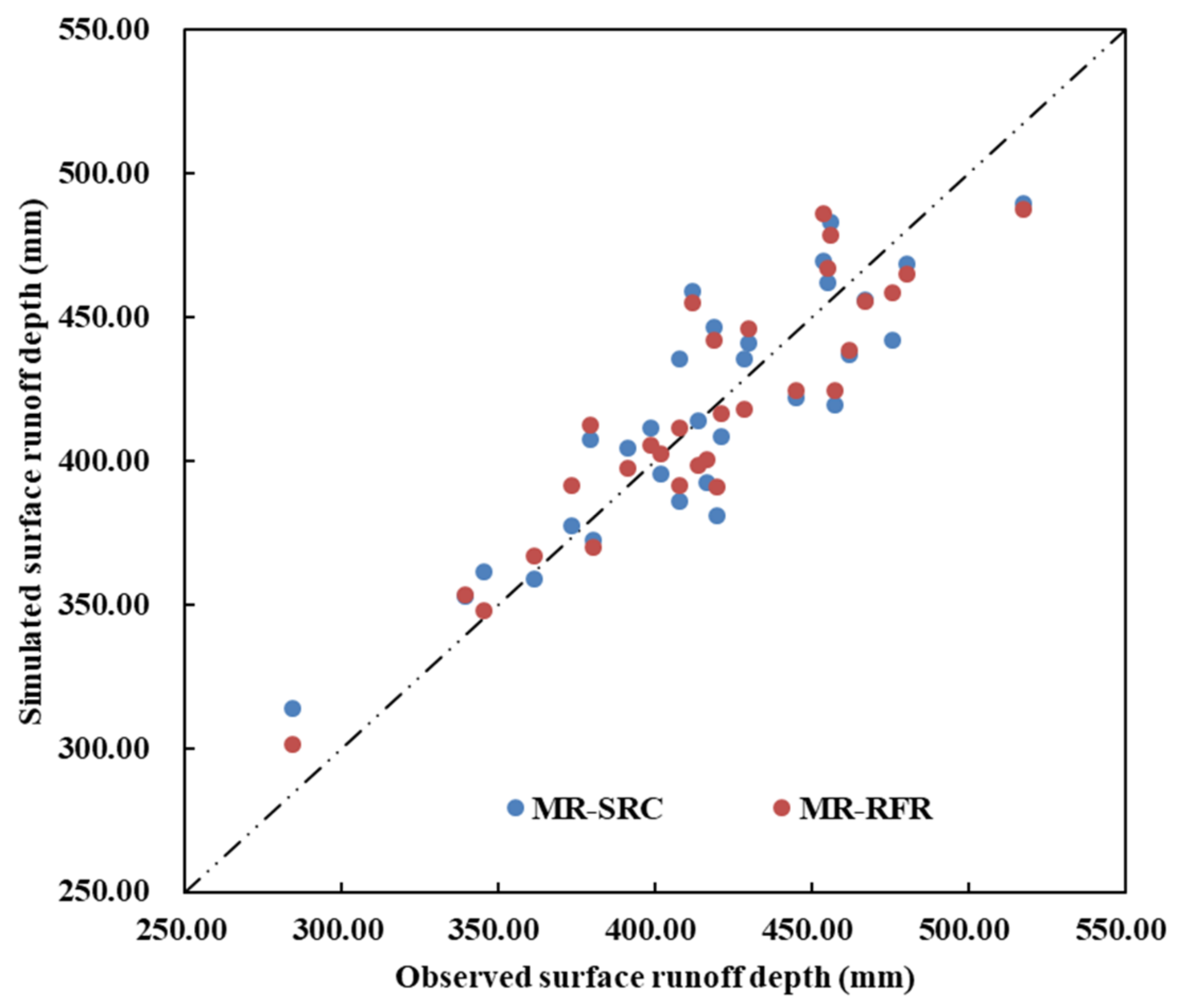
| MRSRC | Surface runoff | Pre | 0.64 | −28.62 | 0.78 | 0.75 | 23.99 |
| R×5day | −0.25 | ||||||
| TR | −1.47 | ||||||
| MRRFR | Surface runoff | Pre | 0.73 | 278.24 | 0.82 | 0.80 | 21.29 |
| R×5day | 0.49 | ||||||
| Tem | −41.21 |
| 1985–2014 | 2036–2065 | 2071–2100 | |||||||
|---|---|---|---|---|---|---|---|---|---|
| MAR (mm) | ZMK | Slope (mm/Decade) | MAR (mm) | ZMK | Slope (mm/Decade) | MAR (mm) | ZMK | Slope (mm/Decade) | |
| Historical period | 416.82 | −1.41 | −14.43 | ||||||
| SSP1-2.6 | 467.22 | −2.32 | −9.46 | 469.27 | 1.97 | 7.99 | |||
| SSP2-4.5 | 450.79 | −0.46 | −3.57 | 445.31 | 1.43 | 9.15 | |||
| SSP3-7.0 | 453.75 | −1.36 | −6.71 | 453.80 | 0.32 | 2.35 | |||
| SSP5-8.5 | 440.87 | −1.32 | −11.06 | 442.72 | 1.64 | 8.89 | |||
Disclaimer/Publisher’s Note: The statements, opinions and data contained in all publications are solely those of the individual author(s) and contributor(s) and not of MDPI and/or the editor(s). MDPI and/or the editor(s) disclaim responsibility for any injury to people or property resulting from any ideas, methods, instructions or products referred to in the content. |
© 2023 by the author. Licensee MDPI, Basel, Switzerland. This article is an open access article distributed under the terms and conditions of the Creative Commons Attribution (CC BY) license (https://creativecommons.org/licenses/by/4.0/).
Share and Cite
Wan, H. Projection of Future Climate Change and Its Influence on Surface Runoff of the Upper Yangtze River Basin, China. Atmosphere 2023, 14, 1576. https://doi.org/10.3390/atmos14101576
Wan H. Projection of Future Climate Change and Its Influence on Surface Runoff of the Upper Yangtze River Basin, China. Atmosphere. 2023; 14(10):1576. https://doi.org/10.3390/atmos14101576
Chicago/Turabian StyleWan, Hanli. 2023. "Projection of Future Climate Change and Its Influence on Surface Runoff of the Upper Yangtze River Basin, China" Atmosphere 14, no. 10: 1576. https://doi.org/10.3390/atmos14101576