TimesNet-PM2.5: Interpretable TimesNet for Disentangling Intraperiod and Interperiod Variations in PM2.5 Prediction

Abstract

Time-series forecasting has a wide range of application scenarios. Predicting particulate matter with a diameter of 2.5 μm or less (PM2.5) in the future is a vital type of time-series forecasting task where valid forecasting would provide an important reference for public decisions. The current state-of-the-art general time-series model, TimesNet, has achieved a level of performance well above the mainstream level on most benchmarks. Attributing this success to an ability to disentangle intraperiod and interperiod temporal variations, we propose TimesNet-PM2.5. To make this model more powerful for concrete PM2.5 prediction tasks, task-oriented improvements to its structure have been added to enhance its ability to predict specific time spots through better interpretability and meaningful visualizations. On the one hand, this paper rigorously investigates the impact of various meteorological indicators on PM2.5 levels, examining their primary influencing factors from both local and global perspectives. On the other hand, using visualization techniques, we validate the capability of representation learning in time-series forecasting and performance on the forecasting task of the TimesNet-PM2.5. Experimentally, TimesNet-PM2.5 demonstrates an improvement over the original TimesNet. Specifically, the Mean Squared Error (MSE) improved by 8.8% for 1-h forecasting and by 22.5% for 24-h forecasting.

1. Introduction

Particulate matter (PM) with a diameter of 2.5 μm or less, known as PM2.5, poses a significant threat to human health due to its ability to infiltrate the respiratory system and contribute to various respiratory and cardiovascular illnesses [1]. In 2023, the global focus on PM2.5 concentrations intensified due to rising pollution levels and the alarming effects PM2.5 had on public health. Multiple studies have been conducted this year, shedding light on various aspects of PM2.5 and their broader implications. Data with different characteristics were separately predicted using appropriate models and the final, combined model results that were obtained were the most satisfactory, according to Ban et al. [2]. The high accuracy of the proposed method [3] was verified by actual PM2.5 data from Beijing, China, which provides an effective method for predicting PM2.5 concentration. Wang et al. [4] presented certain limitations when it came to deeply mining the joint influence of multiple monitoring sites and their inherent connections with meteorological factors.

Predicting PM2.5 concentrations for the year 2023 and in the near future is crucial as it provides a roadmap for potential mitigation strategies, aids policymakers in enacting necessary regulations, and offers the public vital information to protect their health. Accurate forecasting of PM2.5 concentrations is also essential for managing air quality, implementing pollution mitigation strategies, and protecting public health.

In recent years, the application of machine learning (ML) and deep learning (DL) techniques for PM2.5 prediction has gained considerable attention. PM2.5 prediction is approached as a time-series forecasting problem, given the dynamic temporal dependencies observed in pollutant concentrations, which can be influenced by factors ranging from meteorological conditions to anthropogenic activities, according to [5].

However, as illustrated in Figure 1, there are two key points to applying this model to our concrete PM2.5 prediction task. The first is that our task requires the model to predict specific time spots in the future. Consequently, corresponding modifications were implemented on the periodicity selection of the original TimesNet, incorporating four specific time patterns to heighten its time-specific responsiveness. Additionally, the loss function was adapted to intensify its focus on these four critical time spots. The second key point is the feature selectivity of our PM2.5 prediction task. Other than treating it in a static way to compute similarity, we allowed our model to learn further complicated selectivities via the gate we added, which replaced the simple projection. Beyond overall performance, these two improvements to the model allow for greater interpretability by visualizing time variations to reveal potential rules in the PM2.5 time series.

In this study, a modified version of TimesNet, termed TimesNet-PM2.5, is proposed, tailored specifically for the task of PM2.5 forecasting. Through extensive experiments, it becomes evident that TimesNet-PM2.5 outperforms not only the original state-of-the-art TimesNet model, but also other benchmark models such as ARIMA [6] and ST-CCN-PM_2.5 [7], in PM2.5 prediction scenarios across varied prediction lengths, ranging from 1 to 24 h. This consistent enhanced performance underscores the efficacy of the modifications introduced to TimesNet-PM2.5, rendering it a potent solution for PM2.5 forecasting. The salient contributions and innovations are summarized as follows:

• Pivotal enhancements were introduced to the TimesBlock within the TimesNet architecture, specifically integrating targeted temporal patterns and refining time sequence transformation methodologies. Specifically, we incorporated four task-related temporal variations for recognition.
• A more specific loss function was designed to dynamically adjust the learning orientation between general prediction and specific time spots, utilizing an easy-to-hard learning strategy for enhanced forecasting.
• A gate mechanism was introduced in TimesNet that deftly intertwined statistical correlation with PM2.5 and the inherent learning of the model. This dual-aspect approach refined feature selection, ensuring optimal input for the TimesBlock and enhancing PM2.5 time-series projections.
• This redesigned TimesNet boasts great interpretability, allowing for vivid visual explanations of predictions. Notably, its performance surpasses both classical time-series forecasting baselines and the original TimesNet model.

In this study, state-of-the-art meteorological sensors from the Fengtu brand, called the “Fengtu Small-scale Meteorological Station Automatic Microdevice”, were used in data collection. This sensor is not only versatile for applications in agriculture, hydrology, tourist areas, schools, residential communities, and research scenarios, but also boasts a customized monitoring suite to cater to varied situational requirements. The data it can capture include wind speeds, atmospheric pressure, CO concentrations, wind direction, and more. Notably, its probe is ingeniously concealed, a design feature that ensures that there is no obstruction to natural wind flow and prevents rain or snow accumulation, thus preserving the integrity and accuracy of the collected data.

This study is organized as follows: Section 1, titled “Introduction”, provides an in-depth introduction to our specific research subject and the methods adopted. In this section, we shed light on our motivations for designing TimesNet-PM2.5. Section 2, “Related Work”, outlines representative studies that were previously conducted in the realm of PM2.5 prediction. Furthermore, recent advancements in time-series representation learning have been summarized, elaborating on specific models and methods. The section also introduces TimesNet, the foundational model underpinning this research. Section 3 delves into the detailed enhancements made to the TimesNet model, culminating in the TimesNet-PM2.5 model architecture. A thorough description of the sensor used to collect data in this study is also provided. Section 4, titled “Experiments”, primarily highlights the dataset used and other intricate experimental details. It also offers an analytical view of the results obtained. In Section 5, a further dissection of the experimental outcomes is presented, exploring the interpretability of our results complemented by visual demonstrations. Section 6 concludes the findings and insights of this study.

2. Related Works

2.1. Previous Studies on PM2.5 Forecasting

ML techniques have been widely applied to PM2.5 forecasting, with approaches such as support vector regression (SVR) [8], random forests (RF) [9], and STGCN [10] exhibiting promising results. However, these methods often rely on handcrafted features, which may not capture the complex spatio-temporal relationships inherent to PM2.5 data. DL techniques, including convolutional neural networks (CNNs) [11], long short-term memory (LSTM) networks [12], and gated recurrent units (GRUs) [13], have been shown to effectively model complex spatio-temporal dependencies without the need for manual feature engineering. These models have demonstrated superior performance over traditional ML techniques for PM2.5 forecasting. For instance, Li et al. [14] proposed a CNN-LSTM model that leveraged both spatial and temporal information to predict PM2.5 concentrations. Similarly, Zhang et al. [15] introduced a spatio-temporal attention-based GRU model, which outperformed traditional ML models in terms of prediction accuracy. Recent time-series models, such as vector autoregression (VAR) [16], seasonal-trend decomposition using loess (STL-Loess) [17], and the exponential smoothing state space model (ETS) [18], have been extensively utilized for PM2.5 forecasting. In a study by [19], spatio-temporal patterns of PM10 air pollution in Krakow were analyzed using big data from nearly 100 sensors; the research showcased the superior efficacy of the K-means algorithm with dynamic time warping (DTW) over the SKATER algorithm in discerning annual patterns and variations, thereby providing valuable implications for urban planning and public health policymaking. Saiohai et al. [20] employed vertical meteorological factors collected at multiple heights to train machine learning models, specifically multiple linear regression (MLR) and multilayer perceptron (MLP) models, for predicting PM2.5. These models can effectively capture the temporal patterns in PM2.5 data, but often struggle to account for spatial dependencies.

2.2. Time-Series Representation Learning

Time-series representation learning is pivotal in deciphering intricate patterns within sequential data. Lyu et al. [21] ventured into unsupervised representation learning for medical time series, hoping to tap into the potential of vast amounts of unlabeled data and bolster clinical decision making. Despite the copious amount of research on this subject, the absence of a unified model has been a stumbling block to achieving rapid and precise analytics over vast time-series datasets. To bridge this gap, Paparrizos et al. introduced GRAIL [22], a comprehensive framework dedicated to discerning compact time-series representations that maintained the intricacies of a user-defined comparison function. Moving forward, Fan et al. revealed SelfTime [23], a versatile self-supervised time-series representation of learning methodology. It honed in on the intersample and intratemporal relationships within time series to decode the latent structural features in unlabeled data. Emphasizing the nuances of shapelet dynamics and evolutions, Cheng et al. [24] charted a fresh path by intertwining time-series representation learning and graph modeling, presenting two unique implementations. In a parallel stride, Zerveas et al. launched a groundbreaking framework [25] for multivariate time-series representation, drawing inspiration from the transformer encoder architecture. Indeed, although numerous methodologies for time-series representation learning have been proposed, there remains an imperative need for a unified modeling paradigm. This has ushered in the era of transformer-based time-series forecasting, with a myriad of studies being conducted in recent years. LogTrans [26] has been a frontrunner by amalgamating local convolution with the transformer and championing the LogSparse attention. Reformer [27], on the other hand, harnesses the prowess of local-sensitive hashing (LSH) attention. Notably, both models lay their foundations on the vanilla transformer [28], striving to metamorphose the self-attention mechanism into a sparse version. Informer [29] escalates the transformer framework by incorporating KL-divergence-based ProbSparse attention. In pursuit of linear complexity, FEDformer [30] integrates a Fourier-enhanced structure, whereas Pyraformer [31] brings forth a pyramidal attention module, marked by both interscale and intrascale connections. In essence, the realm of time-series representation learning has witnessed a dynamic evolution, navigating through diverse methodologies and aspirations. From explorations into unsupervised learning in the medical domain to the convergence on a unified modeling paradigm, the journey has been intricate. The crescendo seems to be the transformative impact of transformer-based architectures, which have reshaped the contours of forecasting, promising a future where data sequences reveal their mysteries more profoundly than ever before.

2.3. TimesNet

In 2022, a novel method called TimesNet [32] was proposed for time-series analysis, which effectively addressed the challenges associated with modeling temporal variations in 1D time-series data. The authors introduced the TimesBlock as a versatile backbone for time-series analysis, transforming 1D time series into 2D tensors to enhance representational capabilities. This approach allowed for the effective modeling of complex intraperiod and interperiod variations using 2D kernels. Notably, TimesNet has demonstrated state-of-the-art performance in various time-series analysis tasks, including short- and long-term forecasting, imputation, classification, and anomaly detection. This method serves as a valuable reference for our work, as it highlights the benefits of leveraging higher-dimensional representations for time-series analysis.

3. Methodology

3.1. Overview

The goal of TimesNet-PM2.5 was to predict PM2.5 points in the next 1, 6, 12, and 24 h (detailed illustration shown in Figure 1). Therefore, to solve this more targeted problem, two main factors of the problem—specific time spots and features related to PM2.5—were considered. As shown through TimesNet, it is feasible to modify the model for specific time spot predictions, and a specific training objective was designed to optimize this. Regarding feature selection, features were fused by the gate mechanism, which considered correlation to PM2.5 both from a static view and through self-adaptivity of the network.

3.2. Modified TimesBlock

To enhance the TimesNet model to disentangle the intraperiod and intraperiod variation, we added concrete time patterns in TimesBlock (the submodule of TimesNet). The original TimesBlock first applies fast Fourier transform (FFT) to projected time series ${\mathbf{X}}_{\mathbf{1}\mathbf{D}}\in {\mathbf{R}}^{\mathbf{T}\times \mathbf{C}}$, after feature processing in Figure 2. That is,

$$\begin{array}{cc}\hfill \mathbf{A}& =\mathrm{Linear}\left(\mathrm{Amp}\left(\mathrm{FFT}\left({\mathbf{X}}_{1\mathrm{D}}\right)\right)\right)\hfill \end{array}$$

(1)

$$\begin{array}{cc}\hfill \left\{f_1,\cdots ,f_k\right\}& =\underset{f_{*}\in \left\{1,\cdots ,\left[\frac{T}{2}\right]\right\}}{\arg \mathrm{Topk}}\left(\mathbf{A}\right),p_i=⌈\frac{T}{f_i}⌉,i\in \{1,\cdots ,k\}\hfill \end{array}$$

(2)

In Equation (1), $\mathrm{FFT}(·)\mathrm{and}\mathrm{Amp}(·)$ refer to FFT operation and the calculation of amplitude values, respectively. $\mathbf{A}\in {\mathbf{R}}^{\mathrm{T}}$ indicates the calculated amplitude of each frequency, and $\mathrm{Avg}(·)$ is used to average C dimensions. Then, as depicted in Equation (2), the TopK amplitudes and their corresponding period lengths are selected for further modeling. This process is called the period operation. Equation (2) expresses the interperiod-variation time pattern concerned by the learned model. With the aim to add targeted time patterns to our model, we added the frequency of the targeted time periods we planned to predict to the frequency list in Equation (3). The new frequency list is

$$\begin{array}{c}\hfill \left\{f_1,\cdots ,f_k,f_{k+1},\cdots ,f_{k+n}\right\},p_i=⌈\frac{T}{f_i}⌉,i\in \{1,\cdots ,k,\cdots ,k+n\},\end{array}$$

(3)

where $\{f_{k+1},\cdots ,f_{k+n}\}$ is the set of frequencies of n time period of our PM2.5 prediction task. Consequent modeling procedures were the same as the original TimesNet. Following this, we reshaped the 1D time series ${\mathbf{X}}_{\mathbf{1}\mathbf{D}}$ into many 2D stacked time-series fractions, ${\mathbf{X}}_{\mathbf{2}\mathbf{D}}$, according to the frequencies list and corresponding period length. This is shown as

$$\begin{array}{c}\hfill {\mathbf{X}}_{2\mathrm{D}}^{l,i}={\mathrm{Reshape}}_{p_i,f_i}\left(\mathrm{Padding}\left({\mathbf{X}}_{1\mathrm{D}}^{l-1}\right)\right),i\in \{1,\cdots ,k\}\end{array}$$

(4)

Here, $\mathrm{Padding}(·)$ is used to fill zeros in the temporal dimension to ensure it is divisible for ${\mathrm{Reshape}(·)}_{P_i,f_i}$, and $p_i$ and $f_i$ represent the number of rows and columns of the transformed 2D tensors, respectively. Hence, these 2D tensors carry the pattern of interperiod variation in rows and the pattern of intraperiod variation in the columns of rows. After reshaping, we placed the 2D tensors in convolution networks (we chose the $Inception$ network [33]). Then, we reshaped the 2D tensor transformed by previous convolution networks. Given the original length, we employed truncation to recover it. This process can be described by the following equations ($\mathrm{Trunc}(·)$ is the truncation operation):

$$\begin{array}{cc}\hfill {\widehat{\mathbf{X}}}_{2\mathrm{D}}^{l,i}& =\mathrm{Inception}\left({\mathbf{X}}_{2\mathrm{D}}^{l,i}\right),i\in \{1,\cdots ,k\}\hfill \end{array}$$

(5)

$$\begin{array}{cc}\hfill {\widehat{\mathbf{X}}}_{1\mathrm{D}}^{l,i}& =\mathrm{Trunc}\left({\mathrm{Reshape}}_{1,\left(p_i\times f_i\right)}\left({\widehat{\mathbf{X}}}_{2\mathrm{D}}^{l,i}\right)\right),i\in \{1,\cdots ,k\}\hfill \end{array}$$

(6)

$$\begin{array}{c}\hfill \begin{array}{cc}\hfill {\widehat{\mathbf{A}}}_{f_1}^{l-1},\cdots ,{\widehat{\mathbf{A}}}_{f_k}^{l-1}& =\mathrm{Softmax}\left({\mathbf{A}}_{f_1}^{l-1},\cdots ,{\mathbf{A}}_{f_k}^{l-1}\right)\hfill \\ \hfill {\mathbf{X}}_{1\mathrm{D}}^l& =\sum _{i=1}^k{\widehat{\mathbf{A}}}_{f_i}^{l-1}\times {\widehat{\mathbf{X}}}_{1\mathrm{D}}^{l,i}\hfill \end{array}\end{array}$$

(7)

Finally, we kept the same design of adaptive aggregation and residual connection of TimesNet. Note that $l\to l-1$ refers to the relation to the next layer in Equation (4). Amplitudes reflect the different importance of diverse interperiod patterns; thus, the adaptive aggregation in Equation (5) integrated them into more holistic intraperiod patterns.

3.3. Specific Loss

To enhance the ability of our model to predict specific periods in the future, a specific training objective was applied to lead the model learning it. This loss was composed of the overall predicting part and the specific predicting part. The overall predicting part learned the normal ability in long-period forecasting tasks by mean squared error loss ($\mathrm{MSELoss}(·)$). The only discrepancy of the specific predicting part was that we only counted specific time spots into mean squared error loss. By, respectively, multiplying factor $\mathbf{\Lambda },(\mathbf{1}-\mathbf{\Lambda })$, these two parts were summed up to make up the training objective. That is,

$$\begin{array}{cc}\hfill \mathcal{L}& ={\mathcal{L}}_{all}+{\mathcal{L}}_{part}\hfill \end{array}$$

(8)

$$\begin{array}{cc}\hfill & =\mathbf{\Lambda }·\mathrm{MSELoss}(\mathbf{Y},\widehat{\mathbf{Y}})+(\mathbf{1}-\mathbf{\Lambda })·\mathrm{MSELoss}({\mathbf{Y}}_{\left[\mathbf{slice}\right]},{\widehat{\mathbf{Y}}}_{\left[\mathbf{slice}\right]})\hfill \end{array}$$

(9)

$\mathbf{Y},\widehat{\mathbf{Y}}\in {\mathbf{R}}^{\mathbf{1}\times \mathbf{T}}$ are the true and predicted PM2.5 value series, respectively, and $\left[\mathbf{slice}\right]$ refers to sliced time spots that concern our task. $\mathbf{\Lambda }$ is the hyperparameter for dynamically adjusting the orientation from learning general predicting ability to predicting specific time spots. We tended to initialize it at more than 0.5 at the beginning and let it gradually decrease in practice, which formed the easy-to-hard learning for our model.

3.4. Gate Mechanism for Feature Selection

As demonstrated in Section 1, many factors might not have a significant influence on PM2.5. That results in vital feature selection before we feed input into stacking TimesBlock. Therefore, rather than a simple projection via the original TimesNet, we use the gate mechanism to selectively fuse features pertinent to PM2.5. It can be divided into two parts. One part considers the importance of features to PM2.5 as the statistical correlation about PM2.5. The other part allows our model to learn the relationship by itself. These two parts are added through their respective learnable gating vectors. Our gate design can be mathematically expressed as follows:

$$\begin{array}{c}\hfill {\mathbf{X}}_{\mathbf{1}\mathbf{D}}=\mathsf{œ}\left({\mathbf{Linear}}_{\mathbf{1}}\left(\mathbf{X}\right)\right)\odot \mathrm{Corr}(\mathbf{Y},\mathbf{X})+\mathsf{œ}\left({\mathbf{Linear}}_{\mathbf{2}}\left(\mathbf{X}\right)\right)\end{array}$$

(10)

Here, $\mathbf{X}\in {\mathbf{R}}^{\mathbf{C}\times \mathbf{T}},\mathbf{Y}\in {\mathbf{R}}^{\mathbf{1}\times \mathbf{T}}$ are input C features time series and corresponding PM2.5 value time series, ${\mathbf{Linear}}_{\mathbf{1}},{\mathbf{Linear}}_{\mathbf{2}}\in {\mathbf{R}}^{\mathbf{C}}$ are learnable linear layers, ⊙ is element-wise multiplying, and $mathbf\mathit{\sigma }(.)$ is activating function. Their multiplying to time series is just happening in the feature dimension, which is the broadcasted Hadamard product from the feature dimension, as Figure 2 illustrates. Hadamard products with correlation and activating functions take the role of the gating mechanism, which controls different importances of different features as input.

3.5. Sensor Specifications

Table 1. Specifications of the Fengtu meteorological sensor.

Parameter	Range	Resolution	Accuracy
PM2.5	0–1000 ug/m3	1 ug/m3	±10% (<500 ug/m3)
PM10	0–1000 ug/m3	1 ug/m3	±10% (<500 ug/m3)
TSP	0–1000 ug/m3	1 ug/m3	±10% (<500 ug/m3)
CO (carbon monoxide)	0–10 ppm	0.001 ppm	±5% F.S
SO2 (sulfur dioxide)	0–5 ppm	0.001 ppm	±5% F.S
NO2 (nitrogen dioxide)	0–5 ppm	0.001 ppm	±5% F.S
O3 (ozone)	0–5 ppm	0.1 ppm	±5% F.S
Temperature	−40–60 °C	0.01 °C	±0.3 °C (at 25 °C)
Relative humidity	0–100% RH	0.01% RH	±3% RH
Wind speed	0–60 m/s	0.01 m/s	±0.1 m/s
Wind direction	0–360°	1°	±2°
Atmospheric pressure	30–110 Kpa	0.01 Kpa	$<\pm$4%
Piezoelectric rainfall	0–4 mm/min	0.01 mm	$<\pm$4%
Optical rainfall	0–4 mm/min	0.01 mm	$<\pm$4%
Illuminance	0–20 W LUX	1 lux	$<\pm$3%
Total radiation	0–1800 W/m2	1 W/m2	$<\pm$3%
Noise	30–120 dB	0.1 dB	+1.5 dB
CO2 (carbon dioxide)	400–5000 ppm	1 ppm	±(50 ppm + 5% reading)

provides a detailed overview of the specifications associated with the Fengtu Small-scale Meteorological Station Automatic Microdevice.

In environmental and meteorological studies, meticulous selection of monitoring parameters is crucial for the fidelity and rigor of research outcomes. In this investigation, emphasis is placed on nine key indices: PM10, CO, NO₂, SO₂, atmospheric pressure, humidity, temperature, wind direction, and wind speed, chosen for their pronounced significance in air quality assessments. For instance, PM10, due to its inhalable nature, has been associated with adverse health impacts, while gaseous pollutants like CO, NO₂, and SO₂ are linked to various respiratory and cardiovascular maladies [34]. Furthermore, climatic variables—comprising atmospheric pressure, humidity, and temperature—exert considerable influence on the dispersion and concentration gradients of pollutants [35]. Pertaining to wind speed and direction, they are quintessential determinants governing the propagation and dispersion dynamics of pollutants within the atmospheric milieu [36]. In summation, the selection of these indices strives to furnish a holistic and pragmatic approach for the appraisal and scrutiny of air quality and its attendant environmental repercussions.

4. Experiments

4.1. Dataset and Task

A comprehensive dataset from an array of air monitoring stations strategically positioned across city Haikou in Hainan province was assembled. These stations, as detailed in Figure 3, spread over vital urban sectors such as Xiuying district, Longhua district, Qiongshan district, and Meilan district, among others. This multivariate time series dataset, as outlined in

Table 2. Statistical table of environmental data and Spearman correlation with PM2.5.

	Feature	Statistical Value	Correlation with PM2.5
1	PM10	26 ± 26 ug/m3	0.91
2	CO	0.62 ± 0.75 ppm	0.20
3	NO2	11 ± 12 ppm	0.023
4	SO2	9.9 ± 4.9 ppm	0.043
5	Atmospheric pressure	101 ± 1.00 Kpa	0.31
6	Humidity	60 ± 13% RH	0.008
7	Temperature	30 ± 6.0 °C	−0.25
8	Wind direction	160 ± 87°	−0.092
9	Wind speed	1.02 ± 0.72 m/s	0.13

, encapsulates the PM2.5 readings and several correlated attributes from diverse geographical points.

Given the occasional malfunctioning of sensors, meticulous data quality assurance is vital for researchers. Anomalous values, especially negative air pollutant concentrations or sub-zero temperatures, were deemed outliers and treated accordingly. Missing values spanning less than 12 h were addressed using the Lagrange interpolation method, minimizing data continuity distortion. Using Spearman’s rank correlation coefficient, the significance of each feature in relation to PM2.5 was assessed. This correlation matrix is presented in Table 2. The refined feature set, with their respective correlation scores, was then input into our feature selection mechanism, detailed in Section 3.4.

4.2. Details of Training

4.2.1. Hyperparameters

In practice, we chose 2 layers, 5 highest amplitude of stacked TimesBlock, and 32 as the dimension of tensor processed in our network, which guaranteed the computational efficiency. To achieve the objective of easy-to-hard learning in Section 3.3, we set $\mathbf{\Lambda }$ as 1.0 at the beginning, and planned the linear decreasing to 0.5 at the end of the training. This loss was optimized with Adam optimizer [37] with a learning rate equal to 0.0001.

4.2.2. Metrices

To evaluate the performance of our model, classical time series evaluation matrices were suitable. They were mean squared error (MSE), mean absolute error (MAE), root mean square deviation (RMSE), mean absolute percentage error (MAPE), and mean squared percentage error (MSPE).

4.3. Results

To compare our method, we selected basic ARIMA [6], LSTM [12], LinearRegression [38], RandomForestRegressor [39], GradientBoostingRegressor [39], and SVR [39], as the baselines, and selected TimesNet [32], and our proposed TimesNet-PM2.5 for the experiments. We tried all reasonable hyperparameters for ARIMA using various (p, d, q) combinations and selected the best performance to report. Similarly, for LSTM and other models, we tuned the respective hyperparameters to achieve the best possible performance. For the original TimesNet, we used the same training set of our TimesNet-PM2.5 to train it except loss was replaced with simple MSE loss.

In our comprehensive evaluation on the MeiLan dataset subsets and the entire dataset across various time horizons (

Table 3. Results of experiment. We use bold font to show the best performance. “MeiLan” refers to the results on a subset of MeiLan, and “All” represents the performance of the entire dataset.

Model	ARIMA					LSTM
Metric	MSE	MAE	RMSE	MAPE	MSPE	MSE	MAE	RMSE	MAPE	MSPE
MeiLan 1 h	3.04	1.21	0.21	0.00	0.00	49.39	4.41	7.03	0.17	0.11
MeiLan 6 h	7.89	2.32	2.81	0.06	0.00	96.19	6.81	9.81	0.23	0.09
MeiLan 12 h	26.39	3.90	5.14	0.09	0.01	146.19	8.04	12.09	0.28	0.18
MeiLan 24 h	58.30	6.22	7.64	0.17	0.04	115.97	7.71	10.77	0.30	0.24
MeiLan Avg	23.15	3.16	3.95	0.08	0.02	101.93	6.74	9.93	0.24	0.16
All 1 h	5.48	2.18	2.34	0.18	0.02	54.21	4.53	7.36	0.19	0.06
All 6 h	50.26	6.48	7.08	0.73	0.71	120.16	6.90	10.95	0.33	0.53
All 12 h	52.09	6.85	7.21	0.75	0.72	193.82	9.22	13.91	0.35	0.39
All 24 h	62.39	7.55	7.90	0.90	1.02	160.44	8.07	12.67	0.36	0.44
All Avg	42.55	5.76	6.13	0.64	0.62	132.16	7.18	11.22	0.31	0.36
Model	LinearRegression					RandomForestRegressor
Metric	MSE	MAE	RMSE	MAPE	MSPE	MSE	MAE	RMSE	MAPE	MSPE
MeiLan 1 h	19.68	3.29	4.44	0.31	0.01	20.51	3.38	4.53	0.32	0.02
MeiLan 6 h	19.69	3.29	4.44	0.31	0.01	20.89	3.41	4.57	0.32	0.02
MeiLan 12 h	19.74	3.29	4.44	0.31	0.01	21.00	3.43	4.59	0.33	0.02
MeiLan 24 h	19.75	3.30	4.44	0.31	0.02	21.01	3.44	4.58	0.33	0.02
MeiLan Avg	19.72	3.29	4.44	0.31	0.01	20.86	3.42	4.57	0.32	0.02
All 1 h	13.68	2.18	3.60	0.11	0.06	9.56	1.83	3.01	0.095	0.038
All 6 h	44.38	4.17	6.49	0.23	0.24	37.61	3.87	5.98	0.218	0.276
All 12 h	60.81	4.96	7.60	0.29	0.34	51.68	4.64	7.01	0.266	0.304
All 24 h	85.33	5.86	9.01	0.35	1.61	73.11	5.55	8.33	0.352	1.65
All Avg	51.06	4.29	6.96	0.247	0.57	42.99	3.97	6.39	0.238	0.57
Model	GradientBoostingRegressor					SVR
Metric	MSE	MAE	RMSE	MAPE	MSPE	MSE	MAE	RMSE	MAPE	MSPE
MeiLan 1 h	19.86	3.30	4.46	0.31	0.01	12.96	2.69	3.60	0.10	0.02
MeiLan 6 h	20.03	3.32	4.48	0.31	0.01	1.58	3.39	4.40	0.15	0.04
MeiLan 12 h	19.88	3.31	4.46	0.31	0.01	22.48	4.00	4.74	0.17	0.04
MeiLan 24 h	19.92	3.31	4.46	0.31	0.01	25.12	4.20	5.01	0.19	0.06
MeiLan Avg	19.92	3.31	4.46	0.31	0.01	19.99	3.57	4.47	0.15	0.04
All 1 h	13.25	2.11	3.49	0.11	0.06	9.26	1.78	2.92	0.092	0.037
All 6 h	42.97	4.04	6.28	0.22	0.23	36.42	3.74	5.79	0.212	0.267
All 12 h	58.89	4.80	7.36	0.28	0.33	50.05	4.49	6.79	0.258	0.294
All 24 h	82.63	5.68	8.72	0.34	1.55	70.84	5.37	8.07	0.340	1.60
All Avg	49.44	4.16	6.74	0.239	0.55	41.67	3.85	6.19	0.230	0.55
Model	TimesNet					TimesNet-PM2.5(Ours)
Metric	MSE	MAE	RMSE	MAPE	MSPE	MSE	MAE	RMSE	MAPE	MSPE
MeiLan 1 h	8.17	1.80	2.86	0.15	0.05	4.98	1.32	2.46	0.13	0.03
MeiLan 6 h	8.09	2.01	2.84	0.17	0.06	7.52	1.88	2.74	0.17	0.05
MeiLan 12 h	13.57	2.39	3.68	0.17	0.05	12.74	2.11	3.57	0.18	0.07
MeiLan 24 h	19.73	2.99	4.44	0.27	0.22	20.10	2.84	4.48	0.25	0.12
MeiLan Avg	12.38	2.27	3.46	0.19	0.10	11.83	2.07	3.36	0.18	0.07
All 1 h	20.22	1.95	4.50	0.26	0.47	13.46	1.42	3.67	0.14	0.90
All 6 h	38.30	3.10	6.19	0.41	0.24	24.79	2.47	4.98	0.24	0.32
All 12 h	51.21	3.66	7.16	0.55	0.87	30.33	2.78	5.51	0.29	0.66
All 24 h	64.51	4.08	8.03	0.51	0.55	42.47	3.26	6.52	0.35	1.16
All Avg	43.56	3.20	6.47	0.43	0.69	27.76	2.48	5.16	0.25	0.76

), several insights emerged.

In most metrics, particularly for short-term forecasts such as the 1-h horizon in the MeiLan dataset, ARIMA significantly outperformed LSTM, recording an MSE of 3.04 compared to LSTM’s 49.39. However, ARIMA’s performance dwindled for the 24-h forecast horizon, displaying an MSE of 58.30, though it still maintained a lead against LSTM’s MSE of 115.97. When comparing linear regression to RandomForestRegressor on the MeiLan dataset, the latter showed a slight edge with average MSEs of 20.86 and 19.72, respectively. On the entire dataset, the superiority of RandomForestRegressor was more pronounced, particularly for extended time horizons, exemplified by its All Avg MSE of 42.99 against Linear Regression’s 51.06.SVR generally outperformed GradientBoostingRegressor, notably on the entire dataset. This superiority is illustrated in the All Avg metrics, where SVR secured an MSE of 41.67 compared to 49.44 of GradientBoostingRegressor. Of central importance was the comparative performance of TimesNet and our model, TimesNet-PM2.5. Our proposed model showed a consistently higher performance. For example, in the MeiLan Avg metrics, our model registered the best MSE score at 11.83 against TimesNet’s 12.38. Our method performed the best in eight models. Moreover, when comparing TimesNet-PM2.5 to other models on predicting PM2.5 concentration for the next 1 h from the literature [7], it was evident that our model was superior in terms of MSE, RMSE, and MAE (in

Table 4. Comparison of different models on predicting PM2.5 concentration for the next 1 h.

Models	MSE	RMSE	MAE
AR	5.62	2.37	1.43
MA	10.16	3.19	2.08
ARMA	5.81	2.41	1.45
ANN	6.75	2.60	1.61
GRU	6.23	2.50	1.56
ST-GCN	5.76	2.39	1.44
ST-CCN-PM2.5	3.43	1.85	1.41
TimesNet-PM2.5	4.98	2.46	1.32

). For instance, TimesNet-PM2.5 exhibited an MSE of 4.98, which was better than other models expect ST-CCN-PM_2.5. This underscores the effectiveness and efficiency of our proposed model in predicting values on the MeiLan dataset.

5. Analysis

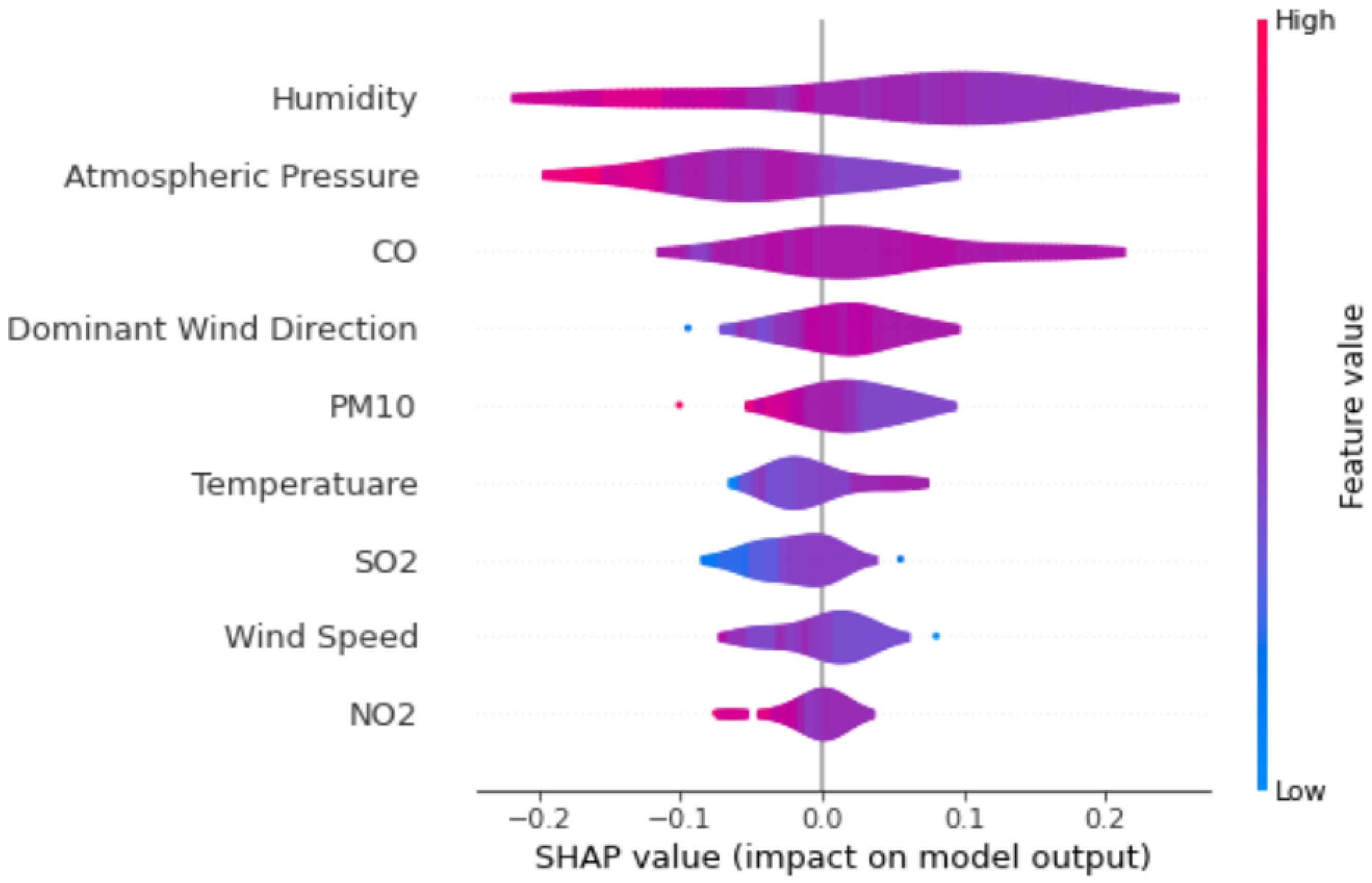
5.1. Feature Importance in Shapley Method

We used the Shapley-based method implemented in [40] to find the most relative factor to PM2.5. Shapley analysis offers a precise quantitative influence rank through feature weight calculation from both local and global perspectives, unlike the qualitative analysis.

Figure 4 illustrates the local perspective of Shapley analysis from a single dataset sample. The horizontal axis of the displayed figure represents the input features, while the vertical axis showcases the SHAP values for the nine features under examination. From a local perspective, “atmospheric pressure” exhibits the most pronounced influence on the variation in PM2.5 concentration. This dominance of atmospheric pressure can potentially be attributed to its integral role in modulating atmospheric stability, which in turn affects the dispersion and concentration of particulate matter. Intriguingly, “CO”, “humidity” and “PM10” manifest equivalent significance in the chart, indicating their equal footing in the determination of PM2.5 fluctuations. The illustration further underscores the nuanced interplay of various environmental factors in shaping PM2.5 dynamics.

Figure 5 delineates the impact weights of input features on output parameters across all samples. The horizontal axis captures the influence weight of a specific feature on the model’s output. Meanwhile, the left vertical axis showcases the array of features under scrutiny, and the right vertical axis employs a diverse color palette to denote the magnitude of feature values. A vertical presentation illustrates the diminishing significance of input feature influence. In this representation, “humidity” emerges as the predominant factor influencing PM2.5 predictions. The heightened influence of humidity can be attributed to its ability to trap particulate matter, reducing its dispersion in the atmosphere, a finding that aligns with the observations made by [41]. Following closely, “atmospheric pressure” stands out as the second most impactful determinant. High atmospheric pressure can lead to stable atmospheric conditions, inhibiting the vertical movement and thus causing the accumulation of PM2.5 near the ground. “CO” holds the third position in terms of its effect on PM2.5 prediction. As CO concentrations surge, there is often a corresponding rise in PM2.5, given that CO emissions often coexist with PM2.5 emissions. This correlation is further underscored by the comprehensive geospatial analyses presented by [41]. When delving deeper, the influence of temperature cannot be overlooked. With a dip in temperature, the predicted PM2.5 values are poised to surge.

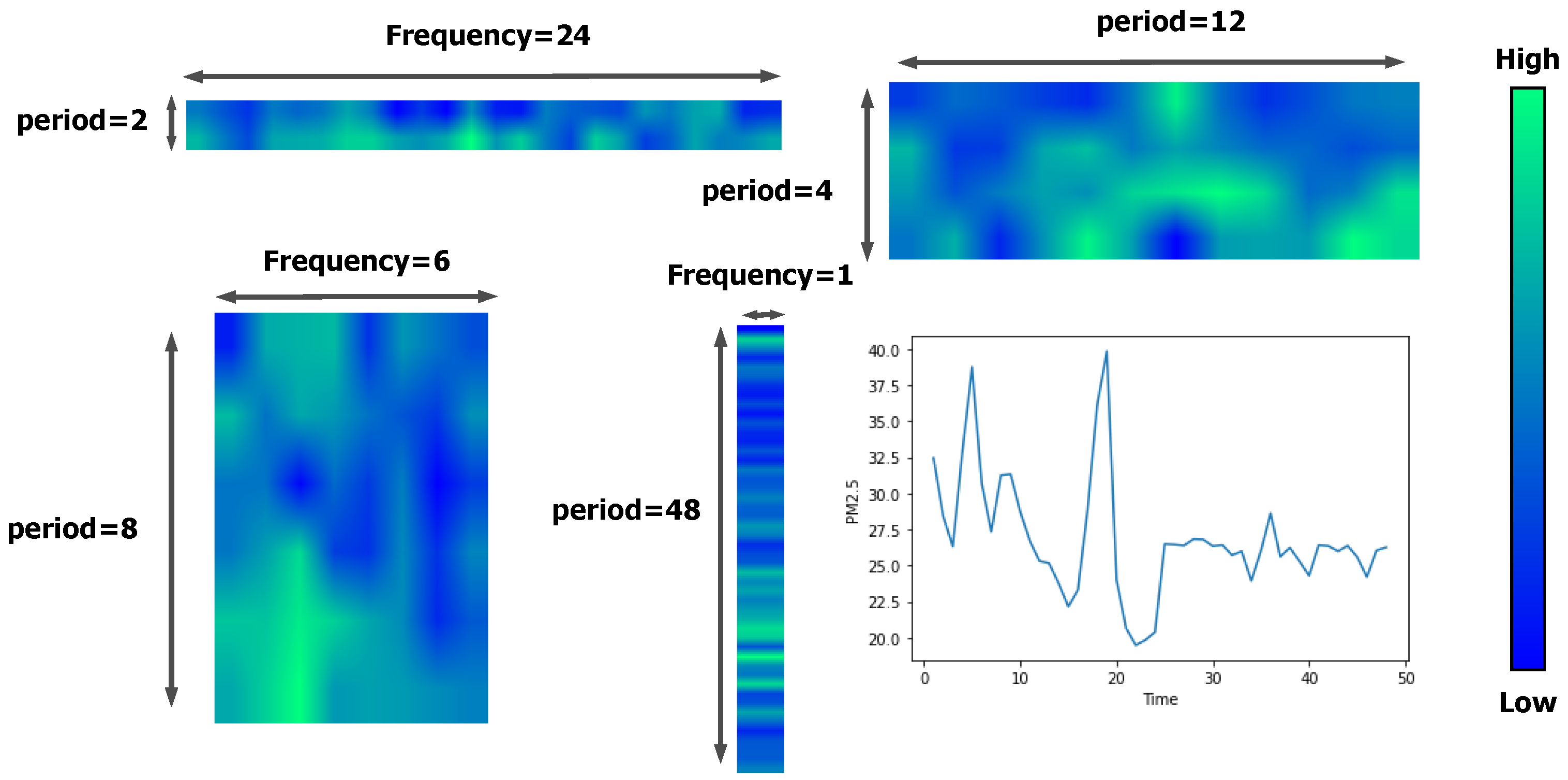
5.2. Temporal 2D-Variations in TimesNet-PM2.5

To elucidate the temporal representations, an illustrative example in the colorful segment of Figure 6 is presented. This visual aid is complemented by the lower segment of the same figure, which manifests the time variations that were predetermined and listed in the frequency list, as expounded in Section 3.2. A meticulous examination of Figure 6 reveals noticeable patterns—certain visual cues display analogous or contrasting trends across different time dimensions, echoing the findings in the case study (See Section 4.6) which highlighted the proficiency of TimesNet [32] in capturing multiperiodicities with precision. Furthermore, taking a cue from the referenced literature, it is insightful that transforming the 1D time series into a 2D spatial configuration, as depicted in Figure 6 and as detailed in Section 3.2, instills a pronounced structural and informational depth. The columns and rows of this transformed tensor resonate with the findings from our cited work [32], encapsulating local inter-relationships between specific time junctures and their overarching periods. Such intricate structuring supports our underlying motivation in opting for 2D kernels, emphasizing the vitality of spatial transformations for efficacious representation learning.

5.3. Future PM2.5 Situation Our Model Predicted

We selected three samples at random from our test dataset for illustration in Figure 7. Upon observation, it became evident that our model delivered a commendable performance. The predicted values closely aligned with the true values, underscoring the model’s capability to offer accurate predictions. Such minor discrepancies between predictions and actual values indicate a reliable and robust model behavior. In addition to our general observations, a more detailed examination of Figure 7 sheds light on the specifics of our model’s performance. In the randomly selected three samples, we presented the juxtaposition of the actual values and the predicted values in subfigures (a), (b), and (c). Visually, the congruence between actual and predicted values is notably pronounced in short-term forecasts, specifically for the 1-h and 6-h predictions. This showcases our model’s acute sensitivity and reliability when forecasting values in the near term. However, as we extend to the 24-h long-term predictions, a slight increase in deviation between the actual and predicted values is observed. While the alignment remains commendable, these minor variations underscore the inherent challenges of forecasting further into the future with the same level of precision.

6. Conclusions

This paper introduces TimesNet-PM2.5, a modified and interpretable version of TimesNet tailored for the PM2.5 prediction problem in Hainan province. The model comprises three innovative modifications on the original TimesNet to the PM2.5 prediction task: specific time patterns associated with the task in the frequency list, a gate mechanism that fuses static similarity with neural selectivity, and a unique loss function. These enhancements ensure that TimesNet-PM2.5 outperforms the original TimesNet and other machine learning and deep learning baseline models in the PM2.5 forecasting task. To investigate the influence of other meteorological indicators on PM2.5 levels, we employed both local and global Shapley models for analysis. The results show that atmospheric pressure exerts the most significant influence on PM2.5 at a local level, while humidity has the greatest impact globally. Interestingly, these findings do not align with the preliminary quantifiable association analysis using the Spearman correlation, indicating the effectiveness of our gate mechanism design for feature selection. Moreover, further delving into visualization analysis, exploring the 2D variation of time series after setting fixed frequency lists and its properties, demonstrate that our model is capable of effective representation learning. It is anticipated that future research endeavors to further magnify interpretability in a holistic manner.

References

1. Lelieveld, J.; Evans, J.S.; Fnais, M.; Giannadaki, D.; Pozzer, A. The contribution of outdoor air pollution sources to premature mortality on a global scale. Nature 2015, 525, 367–371. [Google Scholar] [CrossRef] [PubMed]
2. Ban, W.; Shen, L. PM2.5 Prediction Based on the CEEMDAN Algorithm and a Machine Learning Hybrid Model. Sustainability 2022, 14, 16128. [Google Scholar] [CrossRef]
3. Jin, X.B.; Wang, Z.Y.; Kong, J.L.; Bai, Y.T.; Su, T.L.; Ma, H.J.; Chakrabarti, P. Deep Spatio-Temporal Graph Network with Self-Optimization for Air Quality Prediction. Entropy 2023, 25, 247. [Google Scholar] [CrossRef] [PubMed]
4. Wang, H.; Zhang, L.; Wu, R.; Cen, Y. Spatio-temporal fusion of meteorological factors for multi-site PM2.5 prediction: A deep learning and time-variant graph approach. Environ. Res. 2023. Epub ahead of print. [Google Scholar] [CrossRef]
5. Hu, X.; Belle, J.H.; Meng, X.; Wildani, A.; Waller, L.A.; Strickland, M.J.; Liu, Y. Estimating PM2. 5 concentrations in the conterminous United States using the random forest approach. Environ. Sci. Technol. 2017, 51, 6936–6944. [Google Scholar] [CrossRef] [PubMed]
6. Box, G.E.; Jenkins, G.M. Some recent advances in forecasting and control. J. R. Stat. Soc. Ser. C (Appl. Stat.) 1968, 17, 91–109. [Google Scholar] [CrossRef]
7. Lin, S.; Zhao, J.; Li, J.; Liu, X.; Zhang, Y.; Wang, S.; Mei, Q.; Chen, Z.; Gao, Y. A Spatial–Temporal Causal Convolution Network Framework for Accurate and Fine-Grained PM2. 5 Concentration Prediction. Entropy 2022, 24, 1125. [Google Scholar] [CrossRef] [PubMed]
8. Zhu, S.; Lian, X.; Wei, L.; Che, J.; Shen, X.; Yang, L.; Qiu, X.; Liu, X.; Gao, W.; Ren, X.; et al. PM2. 5 forecasting using SVR with PSOGSA algorithm based on CEEMD, GRNN and GCA considering meteorological factors. Atmos. Environ. 2018, 183, 20–32. [Google Scholar] [CrossRef]
9. Liaw, A.; Wiener, M. Classification and Regression by randomForest. R News 2002, 2, 18–22. [Google Scholar]
10. Han, H.; Zhang, M.; Hou, M.; Zhang, F.; Wang, Z.; Chen, E.; Wang, H.; Ma, J.; Liu, Q. STGCN: A spatial-temporal aware graph learning method for POI recommendation. In Proceedings of the 2020 IEEE International Conference on Data Mining (ICDM), Sorrento, Italy, 17–20 November 2020; pp. 1052–1057. [Google Scholar]
11. Krizhevsky, A.; Sutskever, I.; Hinton, G.E. ImageNet classification with deep convolutional neural networks. In Proceedings of the Advances in Neural Information Processing Systems (NIPS ’12), Lake Tahoe, NV, USA, 3–6 December 2012; pp. 1097–1105. [Google Scholar]
12. Graves, A.; Mohamed, A.R.; Hinton, G. Speech recognition with deep recurrent neural networks. In Proceedings of the 2013 IEEE International Conference on Acoustics, Speech and Signal Processing (ICASSP), Vancouver, BC, Canada, 26–31 May 2013; pp. 6645–6649. [Google Scholar]
13. Chung, J.; Gulcehre, C.; Cho, K.; Bengio, Y. Empirical evaluation of gated recurrent neural networks on sequence modeling. arXiv 2014, arXiv:1412.3555. [Google Scholar]
14. Li, X.; Peng, L.; Yao, X.; Cui, S.; Hu, Y.; You, C.; Chi, T. Long short-term memory neural network for air pollutant concentration predictions: Method development and evaluation. Environ. Pollut. 2018, 231, 997–1004. [Google Scholar] [CrossRef]
15. Zhang, J.; Zheng, Y.; Tong, D.; Shao, M.; Wang, S. Spatio-temporal attention-based gated recurrent unit networks for air pollutant concentration prediction. Atmos. Environ. 2021, 244, 117874. [Google Scholar]
16. Luči’c, P.; Balaž, A. Vector autoregression (VAR) model for exchange rate prediction in Serbia. Industrija 2017, 45, 173–190. [Google Scholar]
17. Derczynski, L.; Gaizauskas, R. Empirical validation of Reichenbach’s tense and aspect annotations. In Proceedings of the 10th Joint ACL—ISO Workshop on Interoperable Semantic Annotation (ISA-10), Reykjavik, Iceland, 26 May 2013; pp. 64–72. [Google Scholar]
18. Svetunkov, I.; Kourentzes, N. Complex Exponential Smoothing State Space Model. In Proceedings of the 37th International Symposium on Forecasting, Cairns, Australia, 25–28 June 2017. [Google Scholar]
19. Zareba, M.; Dlugosz, H.; Danek, T.; Weglinska, E. Big-Data-Driven Machine Learning for Enhancing Spatiotemporal Air Pollution Pattern Analysis. Atmosphere 2023, 14, 760. [Google Scholar] [CrossRef]
20. Saiohai, J.; Bualert, S.; Thongyen, T.; Duangmal, K.; Choomanee, P.; Szymanski, W.W. Statistical PM2.5 Prediction in an Urban Area Using Vertical Meteorological Factors. Atmosphere 2023, 14, 589. [Google Scholar] [CrossRef]
21. Lyu, X.; Hueser, M.; Hyland, S.L.; Zerveas, G.; Raetsch, G. Improving clinical predictions through unsupervised time series representation learning. arXiv 2018, arXiv:1812.00490. [Google Scholar]
22. Paparrizos, J.; Franklin, M.J. Grail: Efficient time-series representation learning. Proc. VLDB Endow. 2019, 12, 1762–1777. [Google Scholar] [CrossRef]
23. Fan, H.; Zhang, F.; Gao, Y. Self-supervised time series representation learning by inter-intra relational reasoning. arXiv 2020, arXiv:2011.13548. [Google Scholar]
24. Cheng, Z.; Yang, Y.; Jiang, S.; Hu, W.; Ying, Z.; Chai, Z.; Wang, C. Time2Graph+: Bridging time series and graph representation learning via multiple attentions. IEEE Trans. Knowl. Data Eng. 2021, 35, 2078–2090. [Google Scholar] [CrossRef]
25. Zerveas, G.; Jayaraman, S.; Patel, D.; Bhamidipaty, A.; Eickhoff, C. A transformer-based framework for multivariate time series representation learning. In Proceedings of the 27th ACM SIGKDD Conference on Knowledge Discovery & Data Mining, Singapore, 14–18 August 2021; pp. 2114–2124. [Google Scholar]
26. Li, S.; Jin, X.; Xuan, Y.; Zhou, X.; Chen, W.; Wang, Y.X.; Yan, X. Enhancing the locality and breaking the memory bottleneck of transformer on time series forecasting. Adv. Neural Inf. Process. Syst. 2019, 32, 4567–4572. [Google Scholar]
27. Kitaev, N.; Kaiser, Ł.; Levskaya, A. Reformer: The efficient transformer. arXiv 2020, arXiv:2001.04451. [Google Scholar]
28. Vaswani, A.; Shazeer, N.; Parmar, N.; Uszkoreit, J.; Jones, L.; Gomez, A.N.; Kaiser, Ł.; Polosukhin, I. Attention is all you need. Adv. Neural Inf. Process. Syst. 2017, 30, 1234–1239. [Google Scholar]
29. Zhou, H.; Zhang, S.; Peng, J.; Zhang, S.; Li, J.; Xiong, H.; Zhang, W. Informer: Beyond efficient transformer for long sequence time-series forecasting. Proc. AAAI Conf. Artif. Intell. 2021, 35, 11106–11115. [Google Scholar] [CrossRef]
30. Zhou, T.; Ma, Z.; Wen, Q.; Wang, X.; Sun, L.; Jin, R. Fedformer: Frequency enhanced decomposed transformer for long-term series forecasting. In Proceedings of the International Conference on Machine Learning, Honululu, HI, USA, 23–29 July 2022; pp. 27268–27286. [Google Scholar]
31. Liu, S.; Yu, H.; Liao, C.; Li, J.; Lin, W.; Liu, A.X.; Dustdar, S. Pyraformer: Low-complexity pyramidal attention for long-range time series modeling and forecasting. In Proceedings of the International Conference on Learning Representations, Virtual, 3–7 May 2021. [Google Scholar]
32. Wu, H.; Hu, T.; Liu, Y.; Zhou, H.; Wang, J.; Long, M. Timesnet: Temporal 2d-variation modeling for general time series analysis. arXiv 2022, arXiv:2210.02186. [Google Scholar]
33. Szegedy, C.; Liu, W.; Jia, Y.; Sermanet, P.; Reed, S.; Anguelov, D.; Erhan, D.; Vanhoucke, V.; Rabinovich, A. Going deeper with convolutions. In Proceedings of the IEEE Conference on Computer Vision and Pattern Recognition, Boston, MA, USA, 7–12 June 2015; pp. 1–9. [Google Scholar]
34. Brook, R.D.; Rajagopalan, S.; Pope, C.A., III; Brook, J.R.; Bhatnagar, A.; Diez-Roux, A.V.; Holguin, F.; Hong, Y.; Luepker, R.V.; Mittleman, M.A.; et al. Particulate matter air pollution and cardiovascular disease: An update to the scientific statement from the American Heart Association. Circulation 2010, 121, 2331–2378. [Google Scholar] [CrossRef]
35. Steinfeld, J.I. Atmospheric chemistry and physics: From air pollution to climate change. Environ. Sci. Policy Sustain. Dev. 1998, 40, 26. [Google Scholar] [CrossRef]
36. Jacobson, M. Fundamentals of Atmospheric Modeling; Cambridge University Press: Cambridge, UK, 2005. [Google Scholar]
37. Kingma, D.P.; Ba, J. Adam: A method for stochastic optimization. arXiv 2014, arXiv:1412.6980. [Google Scholar]
38. Zou, K.H.; Tuncali, K.; Silverman, S.G. Correlation and simple linear regression. Radiology 2003, 227, 617–628. [Google Scholar] [CrossRef]
39. Pedregosa, F.; Varoquaux, G.; Gramfort, A.; Michel, V.; Thirion, B.; Grisel, O.; Blondel, M.; Prettenhofer, P.; Weiss, R.; Dubourg, V.; et al. Scikit-learn: Machine Learning in Python. J. Mach. Learn. Res. 2011, 12, 2825–2830. [Google Scholar]
40. Lundberg, S.M.; Lee, S.I. A unified approach to interpreting model predictions. Adv. Neural Inf. Process. Syst. 2017, 30, 1234–1239. [Google Scholar]
41. Danek, T.; Zaręba, M. The use of public data from low-cost sensors for the geospatial analysis of air pollution from solid fuel heating during the COVID-19 pandemic spring period in Krakow, Poland. Sensors 2021, 21, 5208. [Google Scholar] [CrossRef] [PubMed]
Figure 1. Two key points we addressed to improve the performance of TimesNet for our PM2.5 prediction task. 1. “Specifical Task”: we expect to predict some fixed points of time in the future rather than letting the model find TopK periods in Section 3.2. 2. “Interpretability”: we hope to find the feature that matters most in our PM2.5 prediction task, instead of letting the neural network function as a black box.
Atmosphere 14 01604 g001
Figure 2. TimesNet-PM2.5 architecture: tailored for targeted time spot predictions and optimized PM2.5 feature selection with gate mechanism integration.
Atmosphere 14 01604 g002
Figure 3. The red circle in the top image represents the city of Haikou, which is the location of data sampling. This city is situated in Hainan Province, China. The bottom image displays the distribution of sampling points within the city of Haikou. The observation station is located between longitudes 110 9.6 and 110 32.4 and latitudes 19 57 to 20 0 . The red star in the diagram denotes “MeiLan”. Results pertain to a subset of MeiLan, which is utilized as a subdataset in the following experimental section.
Atmosphere 14 01604 g003
Figure 4. Influence of input features on PM2.5 prediction (from local perspective).
Atmosphere 14 01604 g004
Figure 5. Visualization of applying the Shapley-based method to our model on all data samples (from a global perspective).
Atmosphere 14 01604 g005
Figure 6. Visualization of specific time patterns of one randomly selected example. The line chart represents its PM2.5 value with time. Beyond the line chart, the four rectangles with a blend of bluegreen hues, respectively, represent the four temporal patterns we aim to forecast: future 1, 6, 12, and 24 time units. The 2D tensor mentioned in Section 3.2 is smoothed and visualized using a heatmap representation.
Atmosphere 14 01604 g006
Figure 7. For the randomly selected four samples, we plot the comparison between the actual values and the predicted values, as shown in (ad). The orange line represents the actual values, while the blue line indicates the predicted values. The prediction length is 24, corresponding to the 25–48 h segment in the graph, encompassing the four-time patterns we aim to predict: 1 h, 6 h, 12 h, and 24 h.
Atmosphere 14 01604 g007