Abstract
The Silk Road pattern (SRP) and circumglobal teleconnection pattern (CGT) are two well-known teleconnection patterns, representing the summer circulation variations of the Northern Hemisphere mid-latitudes, which have different definitions but are often regarded as one teleconnection pattern. In view of the distinct features of the SRP/CGT on the interannual (IA) and interdecadal (ID) timescales, the present study investigates the linkages and differences between the SRP and CGT on the two timescales, respectively. On the IA timescale, both the SRP and CGT feature a similar circumglobal wave train structure with strong and significant centers over Eurasia but show clear independence. Specifically, the SRP and CGT illustrate largely the mid-/high-latitude-related and tropics-related parts of the Northern Hemisphere upper tropospheric circulation variations, respectively. Also, the CGT shows a stronger connection to the Indian summer monsoon (ISM) heating and El Niño–Southern Oscillation than the SRP, which makes the CGT more like a tropical forcing-driven atmospheric mode and the SRP more like an internal atmospheric mode. The linkages and differences between them are associated with their asymmetrical relationship during their positive and negative phases, which are attributed mainly to the asymmetrical impact of the ISM heating/cooling on the Eurasian circulations. On the ID timescale, the SRP and CGT are characterized by a coherent two-wave train structure over Eurasia and feature a similar teleconnection pattern over Eurasia, which is associated with the Pacific Decadal Oscillation and Atlantic Multidecadal Oscillation. The present findings on their linkages and differences are helpful in understanding the variability and prediction of the SRP and CGT.
1. Introduction
During the last two decades, two well-known teleconnection patterns have been identified along the Eurasian westerly jet during boreal summer: the Silk Road pattern (SRP) [1,2] and the circumglobal teleconnection pattern (CGT) [3]. The SRP is the leading mode of the upper tropospheric meridional wind anomalies over mid-latitude Eurasia during boreal summer [4,5]. The CGT represents the second leading mode of the upper tropospheric circulation in the Northern Hemisphere (NH), which features a recurrent circumglobal pattern over the NH mid-latitudes [3]. Despite their distinct definitions, the SRP and CGT depict an identical structure, in particular over Eurasia, and are, therefore, often deemed to be the same teleconnection pattern. These two patterns have also been widely investigated due to their great impacts on the NH mid-latitude summer climate variations on both the interannual (IA) and interdecadal (ID) timescales [4,5,6,7,8,9,10,11].
On the IA timescale, the SRP and CGT (referred to as IA-SRP and IA-CGT) are considered as a stationary Rossby wave train along the Eurasian westerly jet that can be self-maintained by extracting kinetic and available potential energy from the basic flow [1,2,12,13,14,15,16]. They can also be modulated or triggered by atmospheric external forcings, such as the tropical Indian summer monsoon (ISM) heating [1,3,17,18], mid-latitude heating over the southern Europe and the eastern Mediterranean [13,19,20], the El Niño–Southern Oscillation (ENSO) [3,15], and the summer North Atlantic oscillation (SNAO) [21]. Furthermore, owing to the changes in the variability of these external forcings, the IA-SRP/IA-CGT structure has experienced remarkable changes around the late 1970s [20] and the late 1990s [22], which are attributed to the changes in the impact of the ISM precipitation on the SRP [20,22,23,24].
On the ID timescale, the SRP (referred to as ID-SRP) shows a different structure from its IA counterpart, characterized by a wave train pattern with a larger meridional scale over Eurasia [25,26]. It also experienced two ID changes (or phase transitions) around the mid/late 1970s and late 1990s, respectively [25,27], which may be associated with the phase shifts of the Pacific Decadal Oscillation (PDO) and the Atlantic Multidecadal Oscillation (AMO). By analyzing the CGT spatial-temporal structure without removing its ID component, Wang et al. [28] pointed out that the CGT reveals evident ID variations with clear weakening around the late 1970s and enhancement after the late 1990s (see Figure 1b), despite the ID-CGT explaining a lower percentage of the NH upper tropospheric circulation variation than the IA-CGT. In addition, Wu et al. [29] identified an ID-CGT pattern along the Eurasian polar jet that resembles the British–Baikal Corridor (BCC) pattern [30] but is different from the conventional CGT.

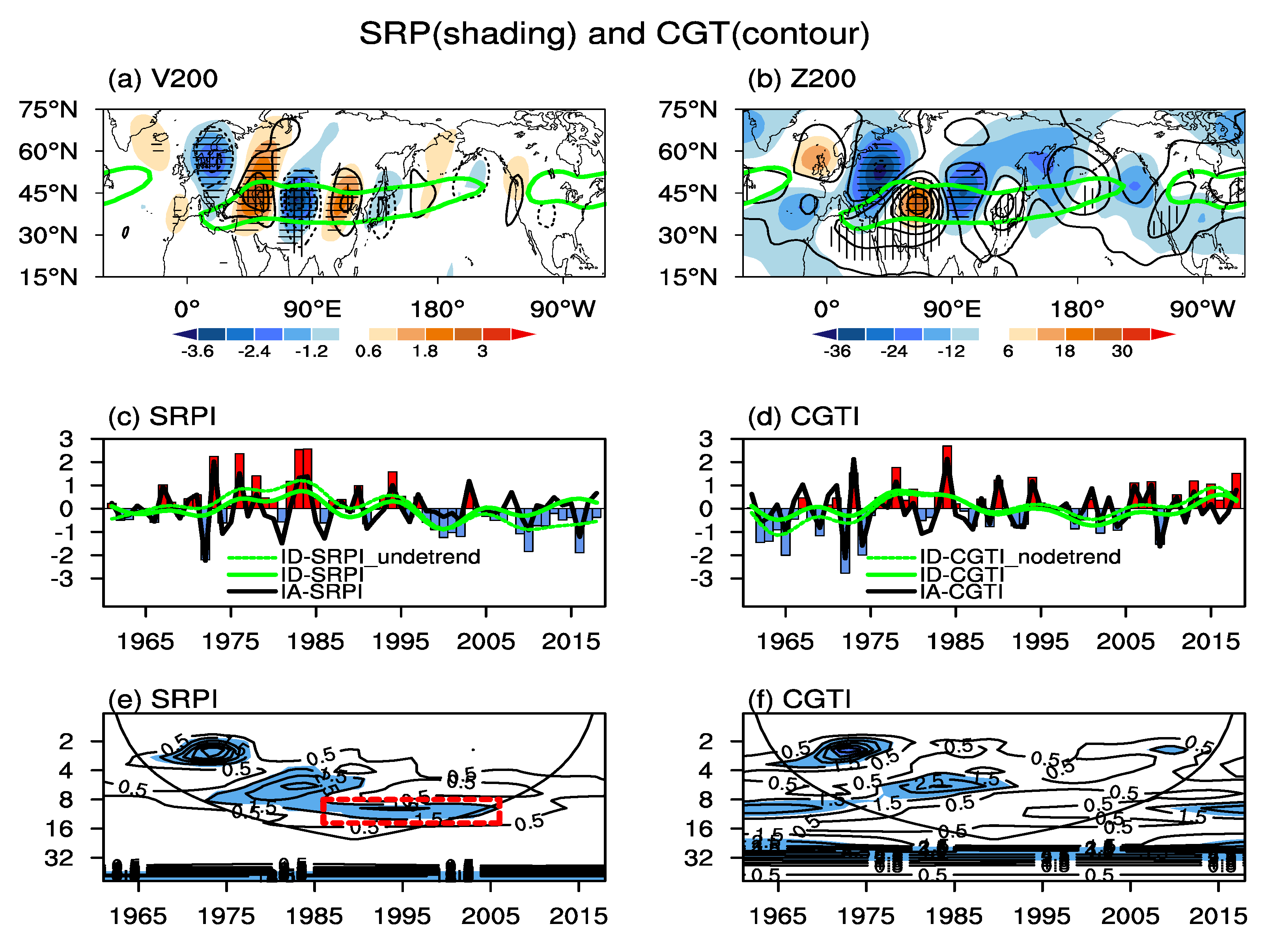
Figure 1.
Summer V200 (a) and Z200 (b) anomalies regressed against the SRPI (shading) and CGTI (contour). The SRPI (c) and (d) CGTI (bar) and their IA component (solid black), detrended ID component (solid blue), and undetrended ID component (dashed blue). The Morlet wavelet spectrum of the SRPI (e) and CGTI (f). The blue contours in (a,b) denote the climatological 200 hPa zonal wind during 1961–2018 with speed exceeding 20 m/s. The horizontal/vertical lines in (a,b) display the V200 (a) and Z200 (b) anomalies significant beyond the 95% confidence level. The units for the V200 and Z200 are ms−1 and gpm, respectively.
Due to their high spatial-temporal similarity [31], most of the previous studies have treated the SRP and CGT as the same teleconnection pattern or regarded the SRP as the Eurasian portion of the CGT, particularly on the IA timescale, and used the names of SRP and CGT alternatively in these studies. However, relatively few works have paid attention to their linkages and differences. Recently, Zhou et al. [31] investigated the linkages and differences between the SRP and CGT using the unfiltered datasets and documented that the SRP is an internally inherent mode in the upper troposphere over Eurasia and the CGT is a section of the SRP over Eurasia continent, which is different from the previous understanding that the SRP is a regional manifestation of the CGT pattern [3]. Given the distinct variations of the two teleconnection patterns on the IA and ID timescales, it is hypothesized that the SRP-CGT relationship may vary on different timescales. Therefore, following Zhou et al. [31], the present study conducts a further investigation on the linkages and differences between the SRP and CGT on both the IA and ID timescales, as well as their associations with the NH summer climate, tropical/extropical heating (precipitation), and global ocean sea surface temperature (SST) anomalies, aiming to provide a comprehensive understanding of the SRP–CGT relationship.
The rest of this paper is organized as follows. Section 2 describes the data and methods. Section 3 revisits the spatial-temporal features of the SRP and CGT on the IA and ID timescales. In Section 4, we investigate the linkages and differences between the two teleconnection patterns on the IA and ID timescales, separately, including the independence of the two teleconnection patterns as well as their links to the NH summer climate, tropical and extra-tropical heating, and global ocean SST anomalies. Section 5 presents the conclusions and a discussion.
2. Data and Method
The monthly observational and reanalysis datasets used in this study include (1) the atmospheric circulation and surface air temperature from the National Centers for Environmental Prediction and Atmospheric Research [32]; (2) the precipitation from the National Oceanic and Atmospheric Administration’s precipitation reconstruction (PREC) dataset [33]; and (3) global SST from the Hadley Centre [34]. Also used are the PDO index and AMO index, which were downloaded from https://www.esrl.noaa.gov/psd/data/correlation/pdo.data (accessed on 15 May 2019) and https://www.esrl.noaa.gov/psd/data/correlation/amon.us.data (accessed on 15 May 2019), respectively. All datasets covered boreal summer (June–July–August, JJA) during 1961–2018, unless otherwise stated.
Regarding the SRP, there are about five different definitions based on different domains (Supplementary Materials Table S1). Different from the other three definitions, the definitions by Lu et al. [1] and Sato and Takahashi [13] focus on the SRP (200 hPa meridional wind; V200) variations mainly over East Asia. In view of the active SRP centers spreading zonally over Eurasia, we select the definition by Yasui and Watanabe [4] that defined the SRP as the first empirical orthogonal function (EOF) mode of the summer mean V200 over the region (20 °N–60 °N; 0°–150 °E) that covers all active centers of the SRP over Eurasia (Figure 1a). The SRP index (SRPI, Figure 1c) is accordingly defined as the normalized first principal component (PC). The SRP accounts for about 28.3% of the total variance of the V200 anomalies, which is highly consistent with the SRP defined by Kosaka et al. [14] and Chen and Huang [15], which is based on slightly different domains (Supplementary Materials Table S1). The results are insensitive to these slight changes.
The CGT is firstly noticed by Ding and Wang [3] on a one-point correlation map of a 200 hPa geopotential height (Z200), which resembles the second EOF of the NH Z200 (see Figure 4b in [3] and Supplementary Materials Figure S1) and the first coupled mode between the unfiltered NH Z200 and tropical precipitation (see Figure 2 in [28]). Therefore, Ding and Wang [3] defined a CGT index (CGTI, Figure 1d) as the Z200 anomalies averaged over the area (35 °N–40 °N; 60°–70 °E) to represent the variations of the CGT, which is widely used in many previous studies. In the present study, we follow Zhou et al. [31] and also use the CGTI with the aim of providing a contrastive analysis. The CGT accounts for about 7.3% of the total Z200 variance over the NH and about 17.4% over the region (20 °N–60 °N; 0°–150 °E), which is lower than the SRP (28.3%), implying a potential difference between the SRP and CGT (Figure 2 and Figure 3).
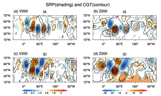
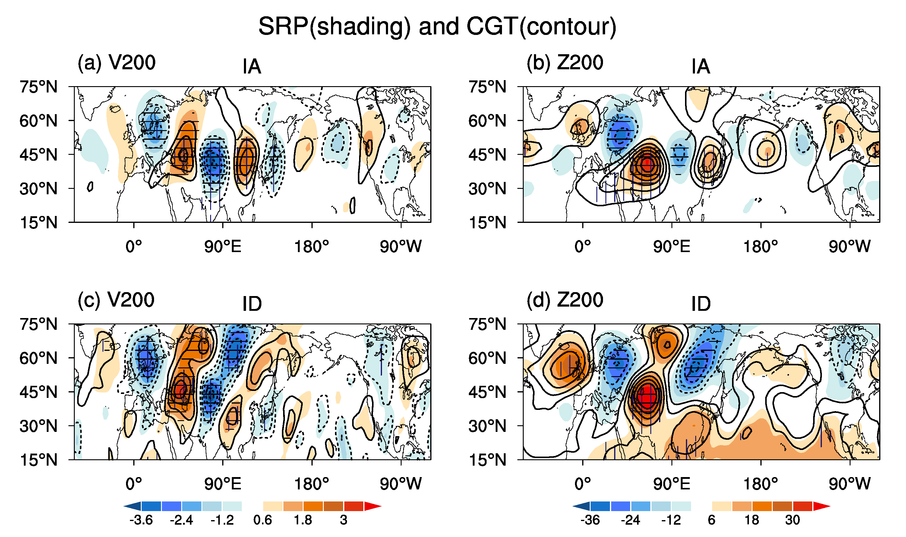
Figure 2.
Summer (a) V200 and (b) Z200 anomalies regressed against the SRPI (shading) and CGTI (contour) on the IA timescale. (c,d) Same as (a,b) but on the ID timescale. The horizontal/vertical lines in (a–d) display that the V200 and Z200 anomalies regressed against the SRPI/CGTI on the IA and ID timescales are significant beyond the 95% confidence level. The units for the V200 and Z200 are ms−1 and gpm, respectively.
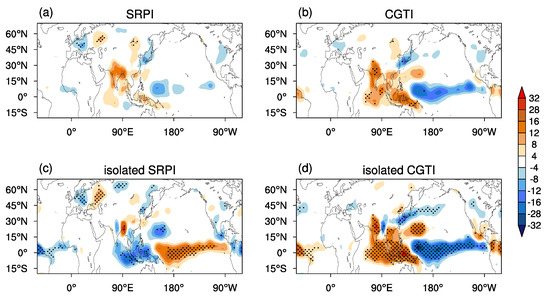
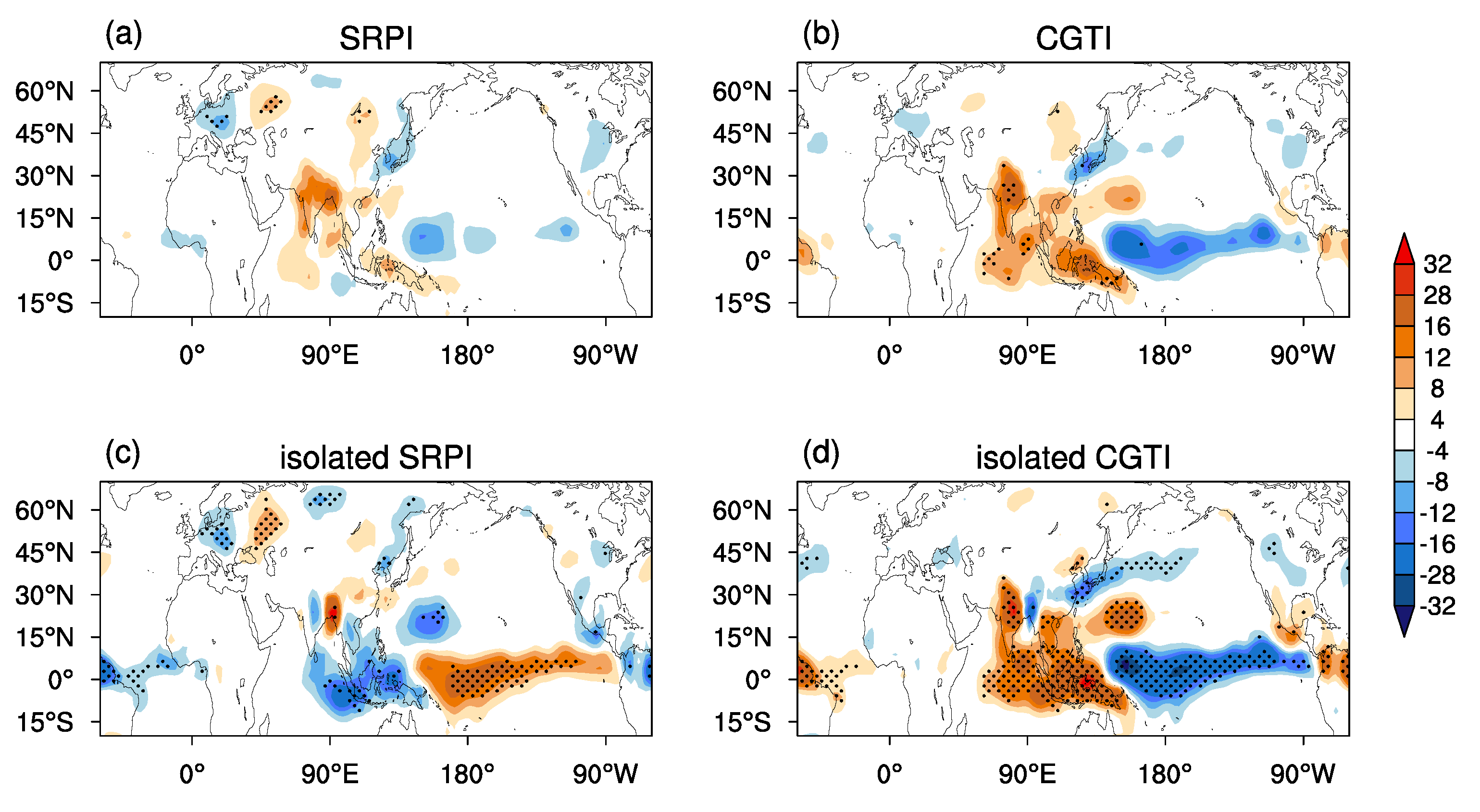
Figure 3.
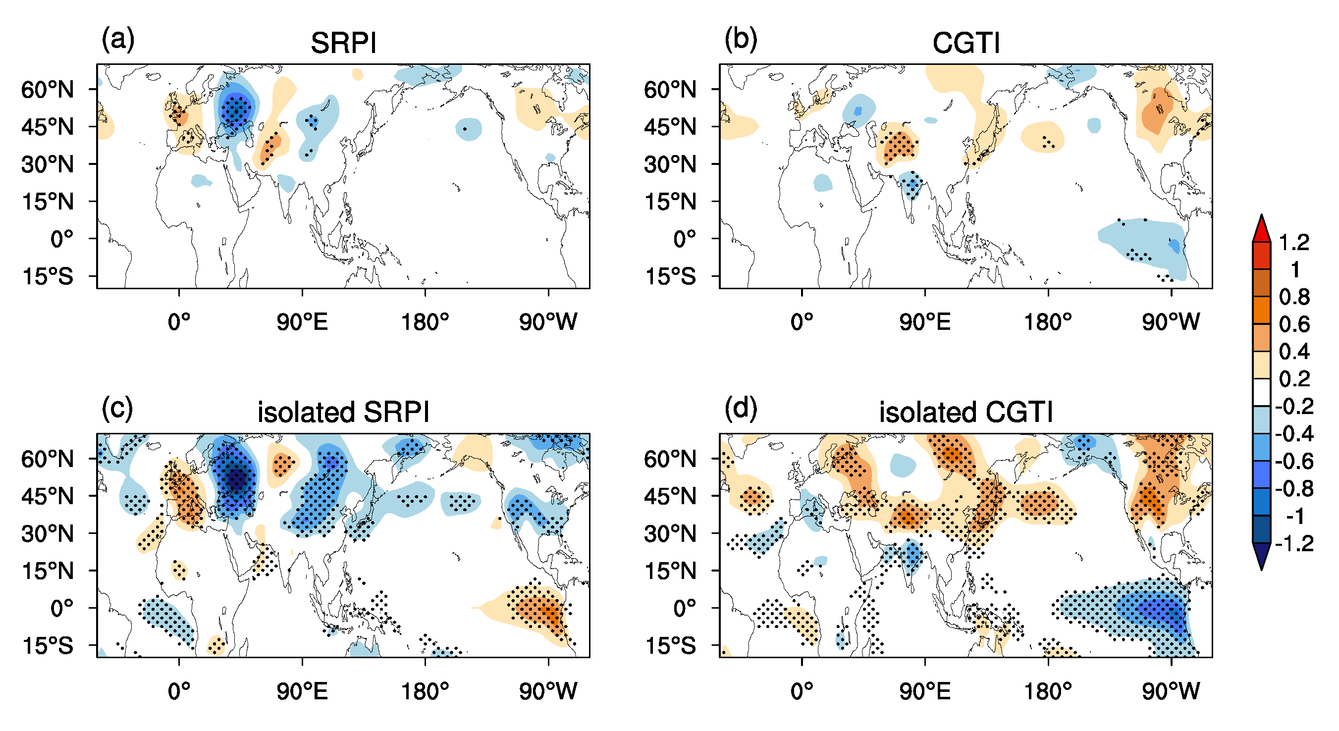
Summer precipitation anomalies (unit: mm/mon) associated with the SRP (a) and CGT (b), as well as with the isolated SRP (c) and the isolated CGT (d) on the IA timescale. Stippling denotes the V200/Z200 anomalies significant beyond the 95% confidence level.
In the following study, we find that the linear trend has an essential impact on the ID variations of the SRP and CGT (Supplementary Materials Tables S2 and S3). Hence, to obtain their IA and ID variations clearly, the linear trend is first removed from the original data and indices. Then, the IA components are extracted from the detrended data/indices using a 9 yr Lanczos high-pass filter [35], and the residual of the detrended data/indices is defined as the ID components. For convenience, the SRP and CGT on the IA and ID timescales are referred to as IA-SRP, IA-CGT, ID-SRP, and ID-CGT, respectively. In addition, the correlation/regression and partial correlation/regression methods are used to investigate their linkages and independence on the IA and ID timescales, as well as their links to the tropical/extra-tropical precipitation and global ocean SST anomalies. For simplicity, their independent parts are termed the isolated SRP and isolated CGT. The confidence level of correlation/regression is estimated by a two-tailed Student’s t-test. The effective degree of freedom is evaluated following Metz [36].
3. Spatial-Temporal Features of the SRP and CGT on the IA and ID Timescales
Given their different definitions, both the V200 and Z200 anomalies related to the SRP and CGT are contrasted, aiming to achieve an intuitive and objective view of the SRP-CGT relationship. To begin, the spatial-temporal features of the total SRP and CGT (not detrended) are provided for comparison.
Figure 1a,b display that the V200/Z200 anomalies regressed onto the total SRPI and CGTI (Figure 1c,d). Corresponding to the total SRP and CGT, both the V200 and Z200 anomalies feature clear circumglobal wave train patterns within the Eurasian westerly jet, with strong and significant active centers over Eurasia. By contrast, the total SRP has stronger negative centers but weaker positive centers than the total CGT. Specifically, in terms of the V200 anomalies, both the total SRP and CGT have five active centers over Eurasia, including two positive ones over Eastern Europe and Eastern China and three negative ones over Western Europe, Central Asia, and Korea–Japan, showing high similarity with a spatial correlation coefficient of 0.87 within the domain (15 °N–75 °N; 0°–360 °E; hereafter the spatial correlation is calculated over this domain unless specified otherwise). One exception is that the total CGT-related anomalies are slightly weaker, and the anomalies in the East Asian portion are situated slightly eastward compared to those related to the total SRP. In terms of the Z200 anomalies, both the total SRP and CGT have four strong active centers over Eurasia, including two positive ones over Central Asia and Eastern Asia and two negative ones over Western Europe and North China, except the negative center related to the total CGT over North China, which extends to eastern Siberia. The spatial correlation coefficient is 0.65 over the NH but increases to 0.72 over the Eurasian portion (15 °N–75 °N; 0–160 °E) in terms of Z200 anomalies. This indicates that the total SRP and CGT reveal a weaker coherence in the Z200 anomalies than in the V200 anomalies. This difference is due to the opposite Z200 anomalies associated with the two patterns over the North Pacific, North America, and North Atlantic.
Figure 1c,d shows the total SRPI and CGTI and their IA and ID components. The SRPI and CGTI are closely interrelated, with correlation coefficients of 0.53, 0.72, and 0.88 on the total, IA, and ID timescales, respectively. For their temporal features, the total SRPI and CGTI reveal significant IA and ID variations (Figure 1c–f). The IA-SRPI (IA-CGTI) accounts for about 57.1% (69.8%) of the total variance of the total SRPI (CGTI), and has a prominent periodicity of the 2–4 years before the late 1970s and the 4–8 years during the 1980s to the mid-1990s (Figure 1e,f). The ID-SRPI (ID-CGTI) explains about 13.4% (15.9%) of the total variance of the total SRPI (CGTI) (Supplementary Materials Table S2) and has coherent phase transitions around the mid-1970s, late 1980s, and early 2010s (Figure 1c,d). These results indicate that the SRP and CGT depict largely the IA variability of the NH upper tropospheric circulation.
Here, it should be noted that the phase transition timings and the percentage variances of the detrended ID-SRPI and ID-CGTI are different from in previous studies [25,26]. These discrepancies are due to the fact that the linear trends of the data/indices are not removed in these studies, which greatly influences the ID variations of the two patterns. To prove this, the IA and ID indices of the two patterns are re-extracted without removing their linear trends from the total indices, and the same analyses are performed. When the linear trend is retained, their correlations and percentage variances of IA-SRPI and IA-CGTI remain nearly the same, but ID-SRPI and ID-CGTI alter greatly (Supplementary Materials Tables S2 and S3). Additionally, the non-detrended ID-SRPI shows phase transitions around the mid-1970s and late 1990s rather than the late 1980s, with clear differences from the detrended ID-SRPI since the late 1990s (Figure 1c). These results are consistent with Wang et al. [25]. The non-detrended ID-CGTI exhibits phase transitions around the mid-1970s, the late 1980s, the late 1990s, and the mid-2000s, with amplitude intensified during the periods prior to the late 1970s and after the early 2010s and weakened amplitude during the periods from the late 1980s to the late 2000s (Figure 1d). The percentage variances of the non-detrended ID-SRPI and ID-CGTI increase to 37.3% and 23.8%, respectively. Furthermore, the correlation coefficient between the ID-SRPI and ID-CGTI decreases to about 0.22, far below the 90% confidence level, which is attributed to the opposite linear trend of the total SRP and CGT indices. These contrasting results confirm the strong impact of the linear trend on the ID-SRP and ID-CGT. Therefore, in the following analyses, we investigate the SRP–CGT relationship on the IA and ID timescales based on the detrended data and indices.
Figure 2a displays the V200/Z200 anomalies associated with the IA-SRP and IA-CGT. Compared to the total counterparts, the IA-SRP and IA-CGT are more coherent with spatial correlation coefficients between them of 0.88 and 0.80 in terms of the V200 and Z200 anomalies, respectively. Both show a similar circumglobal wave train over the NH mid-latitudes and have significant and stronger centers over Eurasia, in particular in the Z200 anomalies that exhibit clearer wave train structures. Notably, the Z200 anomalies associated with the IA-SRP differ largely from the total SRP, displaying a clearer wave train structure with negative centers over Western Europe and Northwestern China–Mongolia and positive centers over Central Asia and Eastern Asia (Figure 2b). Furthermore, the Z200 anomalies associated with the IA-SRP and IA-CGT are also accompanied by another wave train over high-latitude Eurasia, albeit the Z200 anomalies are statistically insignificant. In contrast to the IA-CGT, the IA-SRP has stronger and more significant negative centers over Eurasia. This situation is reversed for their positive centers. These results suggest that the IA-SRP has a stronger connection to the circulation anomalies over Europe than the IA-CGT.
The ID-SRP and ID-CGT bear high spatial similarity, with spatial correlation coefficients of 0.97 in both the V200 and Z200 anomalies and reveal notable differences in their total and IA counterparts. As shown in Figure 2c, the associated V200 anomalies display a two-wave train structure over Eurasia: one mid-/low-latitude wave train along the southern part of the westerly jet and another mid-/high-latitude one along the polar jet. The mid-/low-latitude wave train consists of four strong centers over the Caspian Sea, Central Asia, Central China, and Korea–Japan. These centers are situated southward and westward compared to their total and IA counterparts, with a narrower zonal scale and weaker amplitude over Northwest and Central China. The mid-/high-latitude one has four centers along 60 °N, including two strong negative centers over Western Europe and Northern Russia and two positive ones over Eastern Europe and Eastern Siberia. The associated Z200 anomalies also feature a two-wave train structure over Eurasia with a weak wave train and a prominent one situated to the south and north at about 50 °N over Eurasia, respectively (Figure 2d). The prominent one has four strong centers over the North Atlantic, Western Europe, North Russia, and Eastern Siberia, respectively. The weak one consists of two positive centers over West and South China and a weak negative center over Japan. Compared with their total and IA counterparts, the V200/Z200 anomalies are weak, insignificant, and not well organized over the North Pacific and North America, but the negative centers are stronger and situated northward and westward over Western Europe. In addition, it is worth noting that the high-latitude wave train patterns of the V200/Z200 anomalies resemble the BCC pattern [30], indicating potential connections between the ID-SRP and ID BCC.
The SRP and CGT structures mentioned above are consistent with previous findings on the IA timescale but show different features on the ID timescale, as documented by Wang et al. [25] and Hong et al. [26]. The differences are due to the fact that the non-detrended SRP and CGT are similar to the detrended ones on the IA timescale but differ considerably on the ID timescale (Supplementary Materials Figure S2). In addition, the non-detrended ID-SRP and ID-CGT show weaker spatial coherence. These results confirm the necessity of removing the linear trend when studying the ID variations of the SRP and CGT.
4. Relationship between the SRP and CGT on the IA Timescale
4.1. Independent Parts of the IA-SRP and IA-CGT
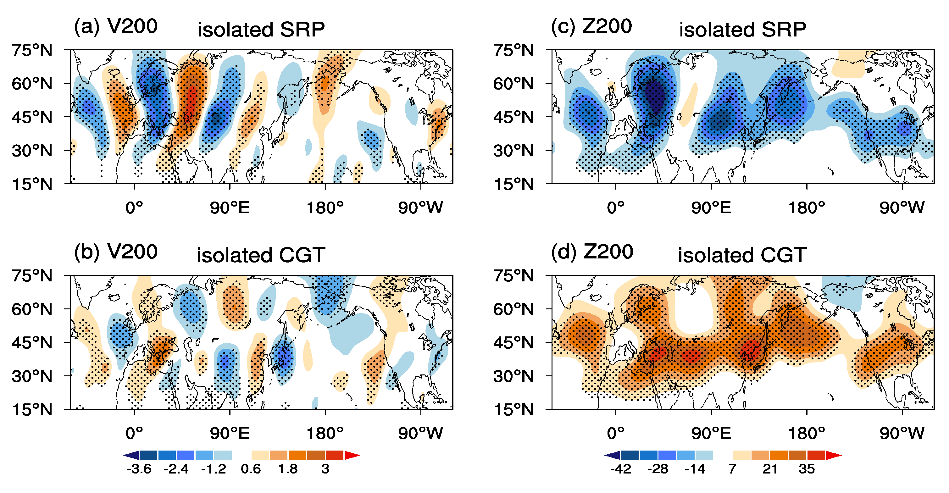
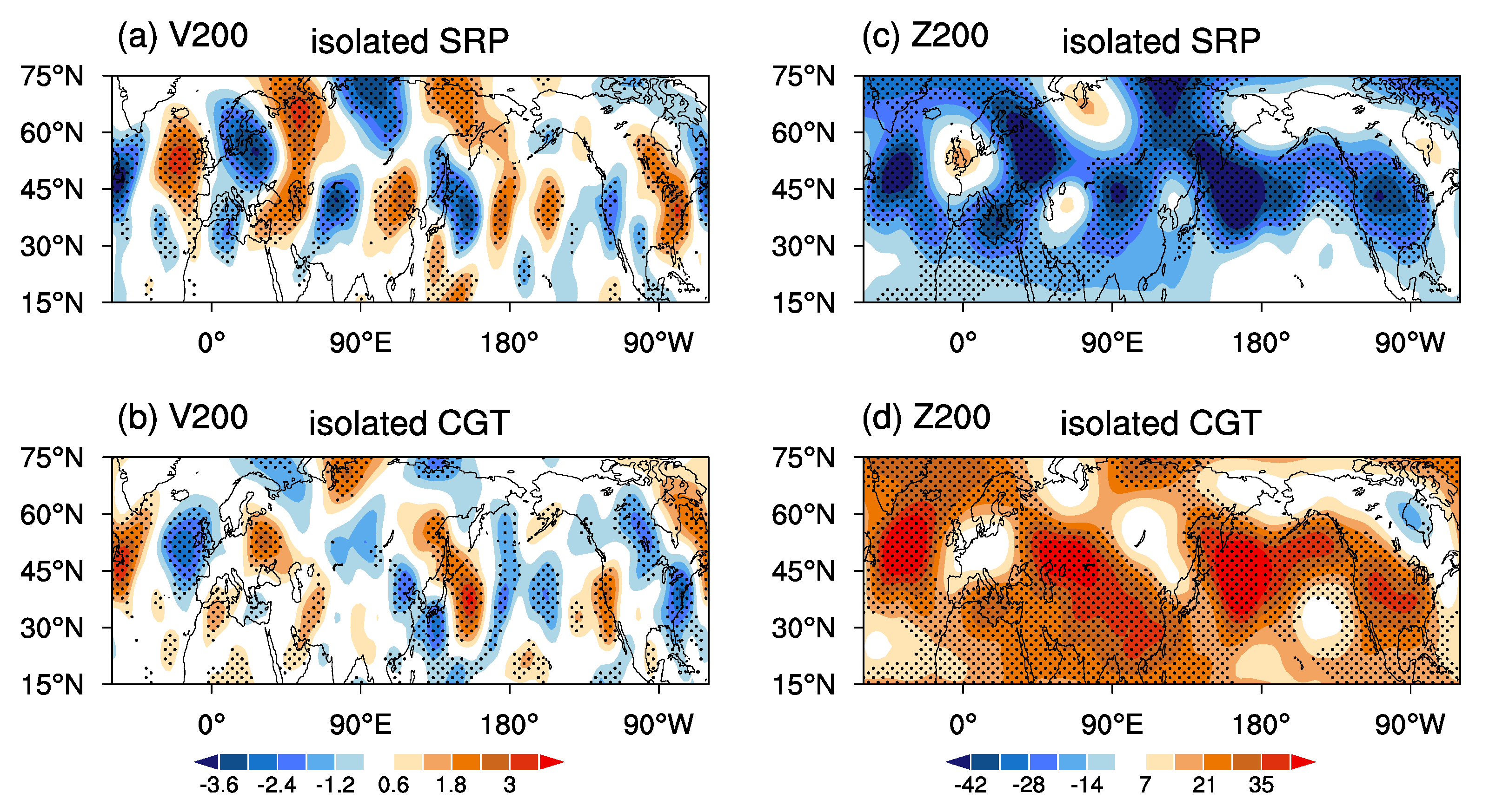
Figure 4 displays the V200 and Z200 anomalies related to the independent parts of the IA-SRP and IA-CGT. In terms of the V200 anomalies, the isolated IA-SRP reproduces the major wave train structure of the IA-SRP with a spatial correlation coefficient of 0.82 between them (Figure 4a). In contrast to the IA-SRP, the isolated IA-SRP is stronger and has a larger meridional scale, with clear enhancement over the high-latitude Eurasia, except that the isolated IA-SRP evidently weakens over Eastern China and Korea–Japan. In addition, the isolated IA-SRP centers move slightly northward and westward over the region from the North Atlantic to Central Asia. The isolated IA-CGT (Figure 4b) shows considerable alternations and has a spatial correlation coefficient of 0.58 with the IA-CGT. Specifically, the isolated IA-CGT is characterized by a notable two-wave train structure over Eurasia. The first wave train is located to the north at about 45 °N along the polar jet with positive centers over Western Europe and Central Russia and negative centers over Eastern Europe and Eastern Siberia, showing opposite structures to those of the IA-CGT and isolated IA-SRP. The second wave train is located to the south at about 45 °N with two strong positive centers over Southern Europe and Eastern China and two strong negative centers over Northwest China and Japan. It is also apparent that the strong positive center of the IA-CGT over the Caspian Sea disappears in the isolated IA-CGT, and the isolated IA-CGT has an opposite structure to the isolated IA-SRP over the North Atlantic, North Pacific, and North America. Despite these differences, the V200 anomalies associated with the isolated IA-CGT match well with those related to the IA-CGT over Eastern Asia, although the V200 anomalies are slightly weaker and move slightly southward and eastward.

Figure 4.
Summer V200/Z200 anomalies associated with the isolated SRP (a,c) and isolated CGT (b,d) on the IA timescale. Stippling denotes the V200/Z200 anomalies with significance beyond the 95% confidence level. The units for the V200 and Z200 are ms−1 and gpm, respectively.
In terms of the Z200 anomalies, the isolated IA-SRP and isolated IA-CGT feature a nearly zonal uniform pattern with almost opposite anomalies over the NH extra tropics (Figure 4c,d), which resembles the extra-tropical circulation responses to ENSO [37,38]. Compared to the IA-SRP (IA-CGT), the isolated IA-SRP (IA-CGT) has much weaker positive (negative) centers and stronger negative (positive) centers that almost overlap with those related to the IA-SRP (IA-CGT), but the strong positive (negative) centers of the IA-SRP (IA-CGT) disappear in the isolated IA-SRP (IA-CGT). The Z200 anomalies related to the isolated IA-CGT resemble the second EOF mode of the Z200 anomalies in the NH, which is defined as the CGT pattern (Figure 4b in [3]) and is also accompanied by another significant wave train over high-latitude Eurasia. The spatial correlation coefficient between the IA-CGT and its independent part is 0.74, which is slightly larger than the IA-SRP with a value of 0.65.
The above results indicate that the isolated IA-SRP/isolated IA-CGT retains the major structure of the IA-SRP/IA-CGT over the northern and southern parts of the NH (to the north and south at about 45 °N), respectively. This is further supported by the spatial correlations between the IA-SRP/IA-CGT and their independent parts within the following two domains of (15 °N–45 °N; 0°–360 °E) and (45 °N–75 °N; 0°–360 °E), particularly in Z200 anomalies (Table 1). These features are different from the findings of Zhou et al. [31], who overlooked the differences between the SRP/CGT on the IA and ID timescales. Along with the results in Section 3, it is apparent that the coherent wave train structures of the IA-SRP and IA-CGT feature a combined result of the isolated IA-SRP and isolated IA-CGT in either the V200 or Z200 anomalies. By contrast, the isolated IA-SRP plays a leading role in the IA-SRP and IA-CGT variations over the NH mid/high latitudes (to the north at 45 °N), while the isolated IA-CGT contributes mainly to the IA-SRP and IA-CGT variations over the NH mid and low latitudes (to the south at 45 °N). Furthermore, it is worth noting that the structures of the isolated IA-SRP and isolated IA-CGT are almost out-of-phase over the North Atlantic, North Pacific, and North America in either the V200 or Z200 anomalies, which can lead to the weak and insignificant centers of the IA-SRP and IA-CGT over these areas (Figure 2a,b).

Table 1.
The spatial correlation coefficients between the IA-SRP/IA-CGT and its independent part in terms of V200 (regular numbers) and Z200 (bold number) anomalies over the domains at (15 °N–45 °N; 0°–360 °E) and (45 °N–75 °N; 0°–360 °E).
4.2. Associations of the IA-SRP and IA-CGT with Global Climate and SST Anomalies
Corresponding to the IA-SRP and IA-CGT, the precipitation anomalies exhibit a similar structure that features a wave train pattern over the NH extra tropics and a zonal dipole pattern over the tropics (Figure 4a,b). In the extra tropics, reduced precipitation is observed over Western Europe, Northern Russia, the Meiyu belt (from the Yangtze River to Korea and Japan), and North America, while enhanced precipitation is seen over Eastern Europe and the areas from North China to Eastern Baikal. In the tropics, above-normal precipitation anomalies are observed over India, the North Indian Ocean, and the Western North Pacific, and below-normal anomalies are apparent over the Central–Eastern tropical Pacific. The Ts anomalies associated with the IA-SRP display a wave train pattern over mid-/high-latitude Eurasia, with warmer Ts over Western Europe, Central Asia to Northern Russia, and North America and colder Ts over Eastern Europe, Northwestern China to Baikal, and Northeastern Russia (Figure 5a). The Ts anomalies in relation to the IA-CGT are characterized by an above-normal zonal pattern along 30 °N–45 °N and a wavy structure to the north at 45 °N, with warmer Ts over Western Europe, Northeastern Russia, and North America and colder Ts over Eastern Europe and Alaska (Figure 5b), but the Ts anomalies are weaker and less insignificant than those related to the IA-CGT. In addition, the IA-CGT also reveals a significant linkage to negative Ts anomalies observed over India and the Eastern tropical Pacific, which are related to the positive ISM heating (Figure 4b) and La Niña-like SST anomalies (Figure 6e–g). The above distributions of the precipitation/Ts anomalies over the mid-/high-latitude NH are consistent with the circulation anomalies related to the IA-SRP and IA-CGT, respectively.

Figure 5.
Like Figure 4 but for Ts anomalies.
Figure 6.
(a–d) Seasonal evolutions of the SST anomalies associated with the SRP (shading) and its independent part (contour) on the IA timescale. (e–h) Like (a–d) but for the CGT (shading) and its independent part (contour). The horizontal lines display the anomalies significant beyond the 95% confidence level.
By contrast, the precipitation/Ts anomalies associated with the IA-SRP are stronger and more significant over mid-/high-latitude Eurasia than those with the IA-CGT, while those associated with the IA-CGT are stronger and more significant over the ISM, tropical Indo-Pacific Ocean, and East Asia. These features are more evident when removing the signal of each counterpart (Figure 4c,d and Figure 5c,d). For example, the precipitation/Ts anomalies related to the isolated IA-SRP retain the main structures of those related to the IA-SRP and show clear intensification over mid-/high-latitude NH but weaken evidently over the East Asian subtropics and shift to opposite anomalies over most parts of the ISM and tropical Indo-Pacific Oceans (Figure 4c and Figure 5c). With respect to the isolated IA-CGT, the precipitation/Ts anomalies resemble those related to the IA-CGT, with stronger and more significant anomalies over most parts of the tropics and NH extra tropics except for Eastern Europe, where positive precipitation/Ts anomalies are observed (Figure 4d and Figure 5d). These features of the precipitation/Ts anomalies are opposite to and have larger amplitude than those related to the isolated IA-SRP. From the above results, it can be concluded that the IA-SRP shows a stronger connection to the precipitation/Ts anomalies over mid-/high-latitude Eurasia, while the IA-CGT shows a stronger connection to the precipitation/Ts anomalies over the ISM, tropical Indo-Pacific Oceans, and East Asia, which can be attributed to the isolated IA-SRP and isolated IA-CGT having a strong connection to the circulation anomalies over the northern and southern parts of Eurasia, respectively.
In addition, the precipitation/Ts anomalies related to the IA-SRP and IA-CGT, as well as their independent parts, feature a response to the La Niña-like or El Niño-like SST anomalies over the tropics (Figure 4a,b and Figure 5a,b). This indicates a linkage of the two IA teleconnection patterns to ENSO [3,14,15,17]. To clarify the differences in their relationships with ENSO, the SST anomalies related to the IA-SRP and IA-CGT, as well as their independent parts, are investigated. As shown in Figure 6e–g, the IA-CGT shows a strong connection with the negative SST anomalies over the Eastern Pacific, which resembles the SST anomaly evolutions of the developing phase of La Niña. This relationship becomes more evident after removing the IA-SRP signal. This is consistent with Ding and Wang [3], who reported that the CGT tends to occur during La Niña developing summers. The La Niña-like SST anomalies favor a decrease in the precipitation/Ts over the tropical Central–Eastern Pacific and an increase in the precipitation/Ts over the ISM, Indian Ocean, and Western Pacific in relation to the (isolated) IA-CGT (Figure 4b,d and Figure 5b,d). The IA-SRP shows a weak connection to the negative SST anomalies over the tropical Eastern Pacific during summer and fall, which is consistent with Lu et al. [1]. The isolated IA-SRP turns to connect strongly to the El Niño-like SST anomalies over the tropical Eastern Pacific during summer and fall (Figure 6a–d), which are opposite to and weaker than the SST anomalies related to the isolated IA-CGT, corresponding to the precipitation/Ts anomalies over the tropical Indo-Pacific Oceans in relation to the (isolated) IA-SRP (Figure 4c and Figure 5c).
The above results indicate that the (isolated) IA-CGT has a stronger connection to the ISM heating anomalies and ENSO than the (isolated) IA-SRP, which are considered key external forcings for the IA-SRP/IA-CGT [1,3,17]. Regarding the (isolated) IA-CGT, the positive Z200 anomalies over Central Asia (Figure 2b and Figure 3d) feature a Gill-type Rossby wave response to the ISM heating forcing [3,17], which can also be excited by divergent flow-induced vorticity advection due to the precipitation anomalies over the tropical Indian Ocean [15]. The weak connection of (isolated) IA-SRP to the ISM heating may be largely attributed to the negative precipitation anomalies over Central–Southern Europe [4,20]. The roles of ENSO-like SST anomalies are significantly observed in the independent parts of the IA-SRP and IA-CGT. The El Niño-like and La Niña-like SST anomalies are responsible for the zonally negative and positive Z200 anomalies related to the isolated IA-SRP and isolated IA-CGT, respectively (Figure 3c,d). There may be two pathways for the La Niña-like SST anomalies affecting the isolated IA-CGT. The first pathway is that the heating anomalies related to La Niña-like SST anomalies can modulate the ISM by triggering the Walker circulation anomalies (figure not shown), which further excites an isolated IA-CGT-like wave train over Eurasia. The second pathway involves the associated heating anomalies forcing a Pacific–North America (PNA) pattern that further excites a wave train over Eurasia and contributes to the isolated IA-CGT (Figure 2b and Figure 3d). The two pathways can often coexist. The second pathway also works for the El Niño-like SST anomalies, influencing the isolated IA-SRP. These results suggest that the IA-CGT is more like a tropical forcing-driven atmospheric mode, while the IA-SRP may be more like an internal atmospheric mode, although it can be modulated by the ISM heating ENSO and mid-latitude disturbances.
4.3. Possible Causes for the Linkages and Differences of the IA-SRP and IA-CGT
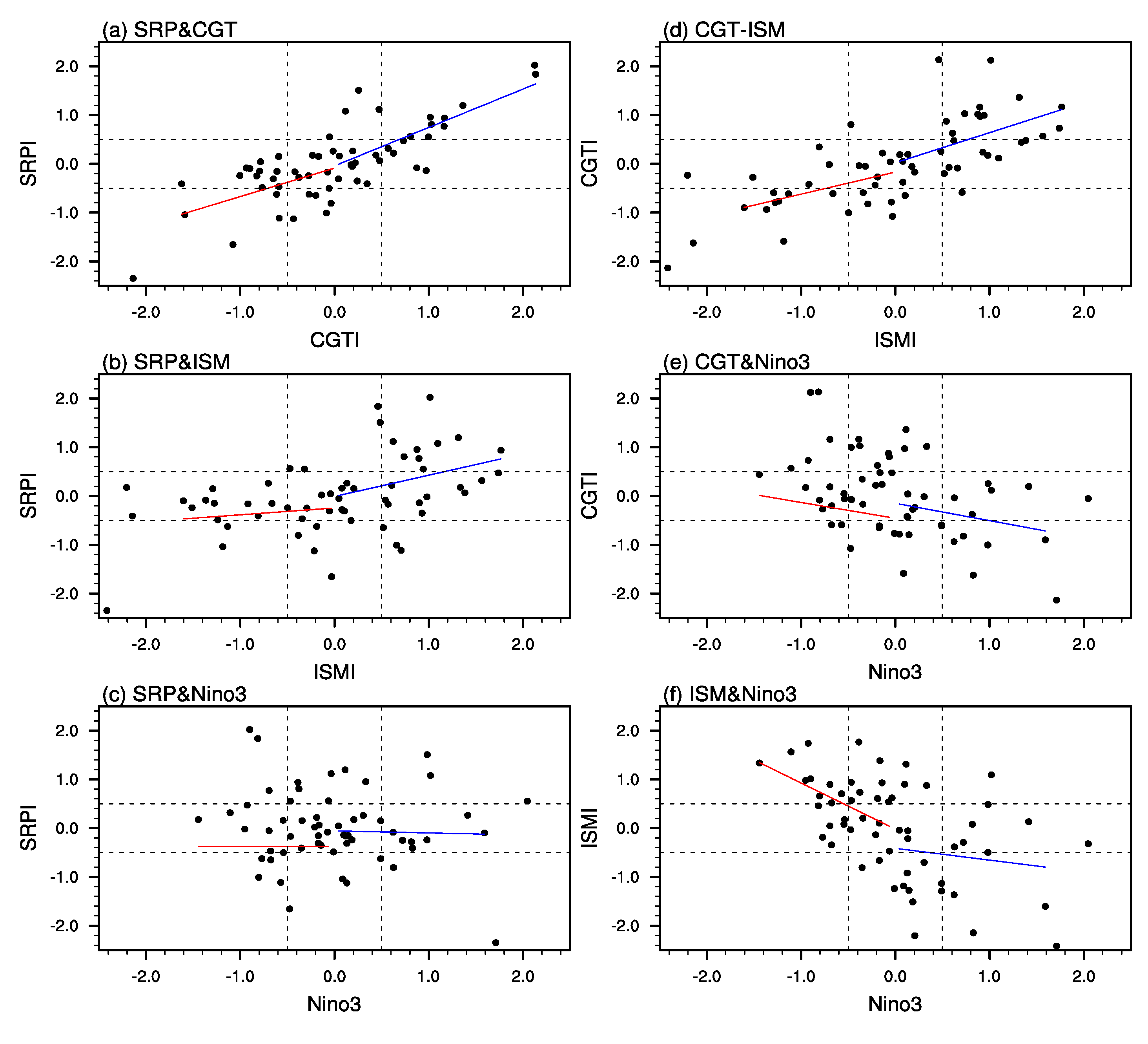
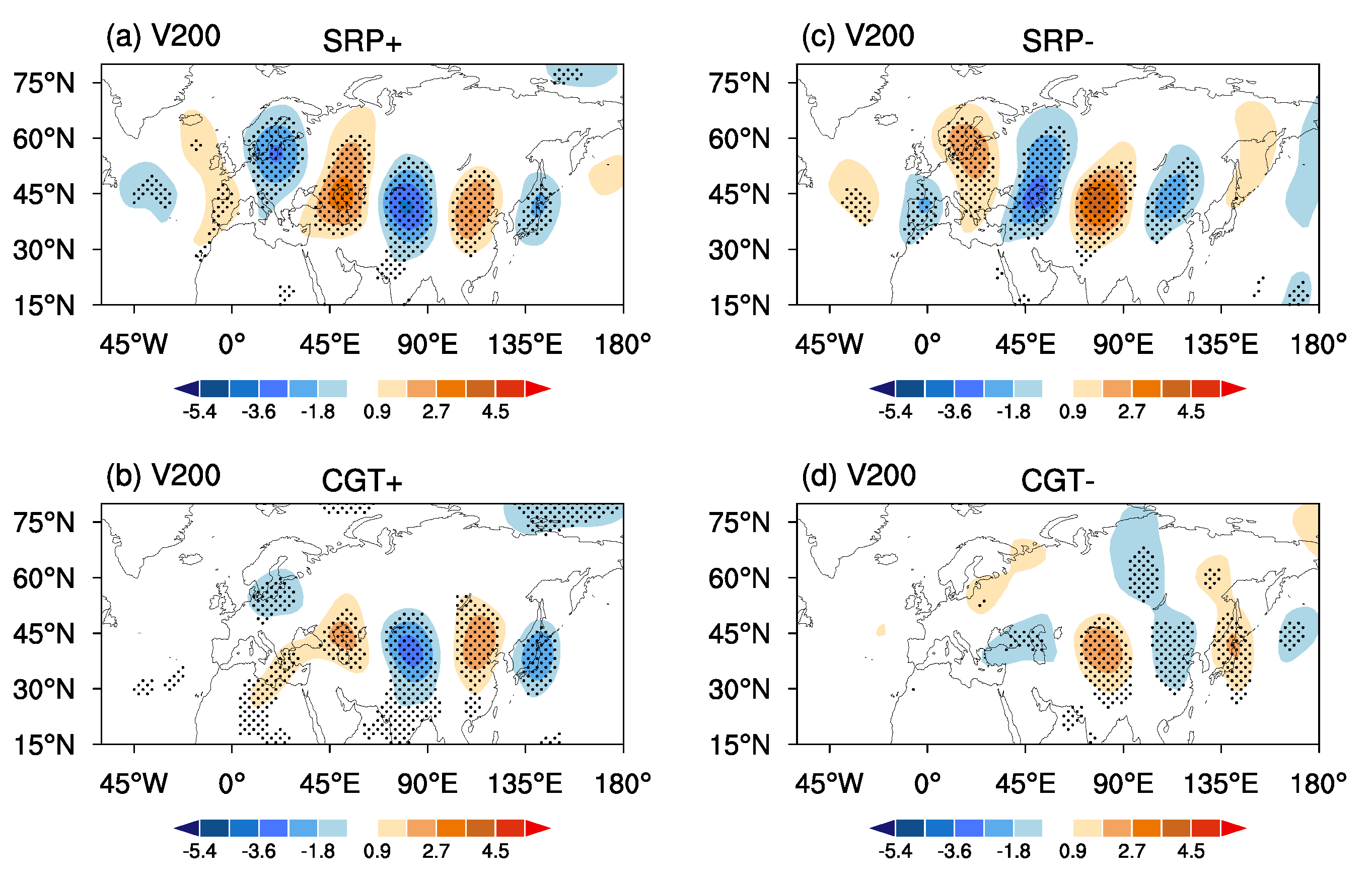
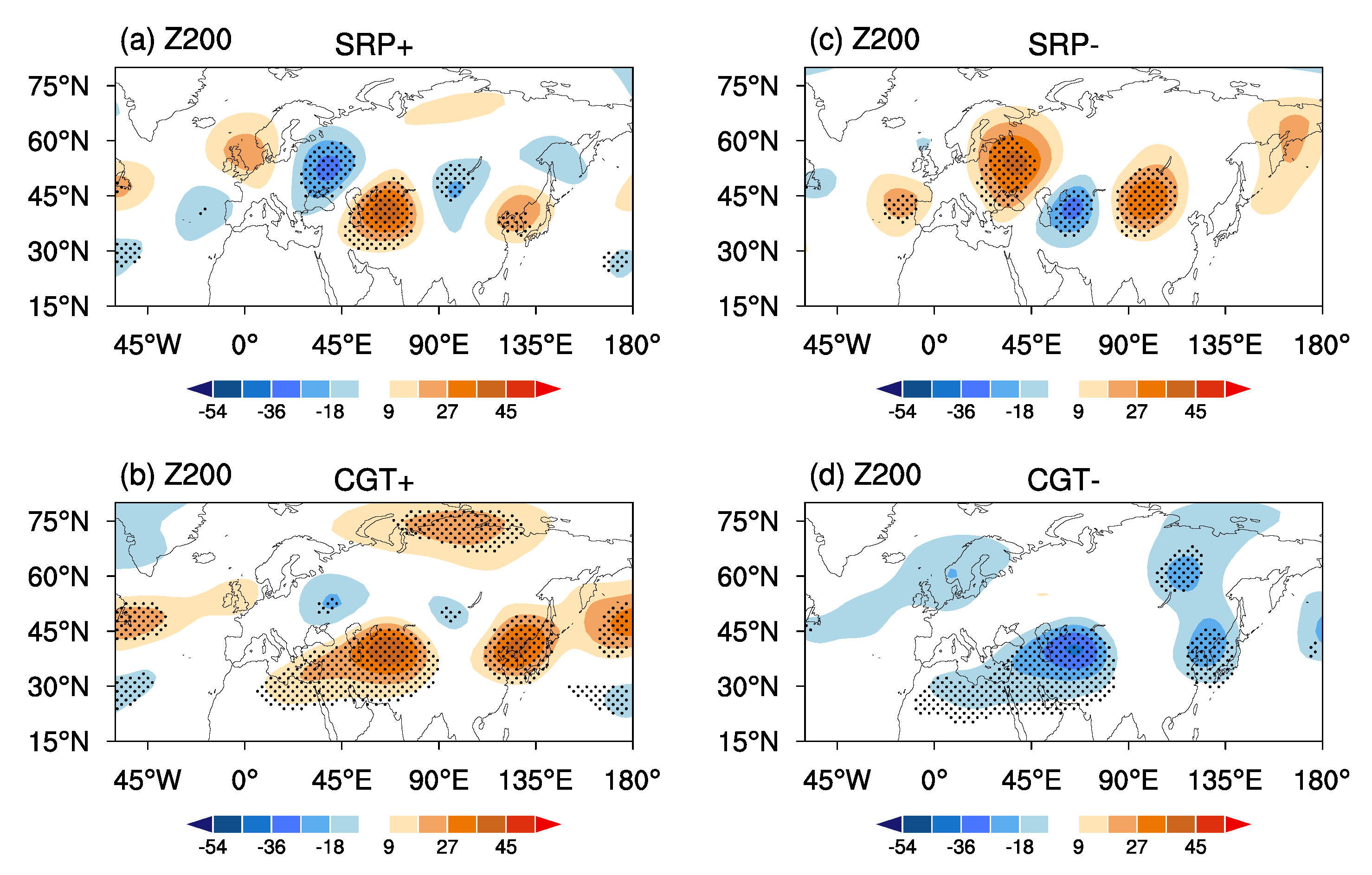
A natural question to ask is why do linkages and differences arise between the IA-SRP and IA-CGT, and what physical factors are responsible for their linkage and difference? Through further analysis, we find that the linkages and differences between the IA-SRP and IA-CGT are associated with their asymmetrical relationship during their positive and negative phases, which are attributed to the asymmetry impacts of the ISM heating and ENSO on NH extra-tropical teleconnections. To verify this, an ISM precipitation index (ISMI) is defined to represent the ISM heating variability, which is the average precipitation anomalies over the domain (15 °N–35 °N; 60°–90 °E), and the Niño3 index is used to denote ENSO, which is the averaged SST anomalies over the domain (5° S–5 °N; 150° W–90° W). With a criterion of 0.5 standard deviations, the typical cases of the IA-SRP and IA-CGT indices and their configurations with the ISMI and Niño3 index are listed in Table 2. Also, a scatterplot between each pair of the IA-SRPI, IA-CGTI, ISMI, and Niño3 index is displayed in Figure 7 to examine their asymmetrical relationship. It can be seen that the IA-SRPI and IA-CGTI are more coherent during their co-positive years than during their co-negative years (Figure 7a), in which there are nine co-positive cases and five co-negative cases. The correlation between them is 0.69 and 0.42 during the two kinds of years, respectively. These features are also supported by the composited V200/Z200 anomalies based on their typical cases. As shown in Figure 8 and Figure 9, the IA-SRP exhibits a symmetrical wave train structure during its positive and negative phases. The IA-CGT shows a weak symmetrical structure and features a similar pattern to the IA-SRP during its positive phase and a different pattern during its negative phase, with notable differences over the North Atlantic and Europe. This configuration makes the IA-SRP and IA-CGT more consistent during their positive phase than during their negative phase, corresponding to their linkages and differences, respectively.
Table 2.
Typical years/cases of different combinations of the IA-SRPI and IA-CGTI (with a criterion of 0.5 standard deviations) and their configurations with the ISMI and Niño3 index. The symbols “+”, “−”, and “neu” after the “SRP” and “CGT” denote the year of the index with values above 0.5, below −0.5, and within ±0.5 standard deviations. The symbols “p” and “n” (“E” and “L”) after the year denote the ISMI (Niño3 index) with values above 0.5 and below −0.5 standard deviations, respectively.
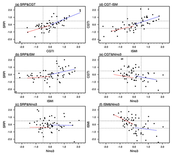
Figure 7.
(a–d) Scatterplot between the (a) SRPI and CGTI, (b) SRPI and ISMI, (c) SRPI and Niño3 index, (d) CGTI and ISMI, (e) CGTI and Niño3 index, and (f) ISMI and Niño3 index. The solid blue (red) line represents the linear regression when the horizontal axis index is larger (less) than zero.

Figure 8.
Composited V200 anomalies (unit: ms−1) during the SRP+ (a), SRP− (c), CGT+ (b), and CGT− (d) years. Stippling denotes the anomalies’ significance beyond the 95% confidence level. The symbols “+” and “−” after the “SRP” and “CGT” denote the year of the IA-SRPI and IA-CGTI with values above 0.5 and below −0.5 standard deviations, respectively.

Figure 9.
Like Figure 8 but for Z200 anomalies (unit: gpm) during the SRP+ (a), SRP− (c), CGT+ (b), and CGT− (d) years.
It is also noticeable that during their strong linkage years, seven out of the nine co-positive cases coexist with positive ISM cases and three out of the five co-negative cases coexist with negative ISM cases (Table 1). This implies that the linkage between the IA-SRP and IA-CGT is closely related to the ISM heating, in particular when the ISM heating is above normal. In addition, the scatterplot between the ISMI, IA-SRPI, and IA-CGTI also shows that the IA-SRP-ISM heating connection presents mainly during positive ISMI years (Figure 7b; with nine co-positives; Table 2). Meanwhile, the IA-CGT-ISM heating connection is evident during both positive and negative ISMI years (Figure 7d; with twelve co-positive and ten co-negative cases; Table 2), which remains evident when excluding the typical IA-SRP cases (with four co-positive and seven co-negative cases; Table 2), corresponding to the strong connection of the (isolated) IA-CGT to the ISM heating. The asymmetry connection of the ISM heating to the IA-SRP and IA-CGT results in the strong linkage between the two teleconnection patterns during their positive phase and weak linkage during their negative phase.
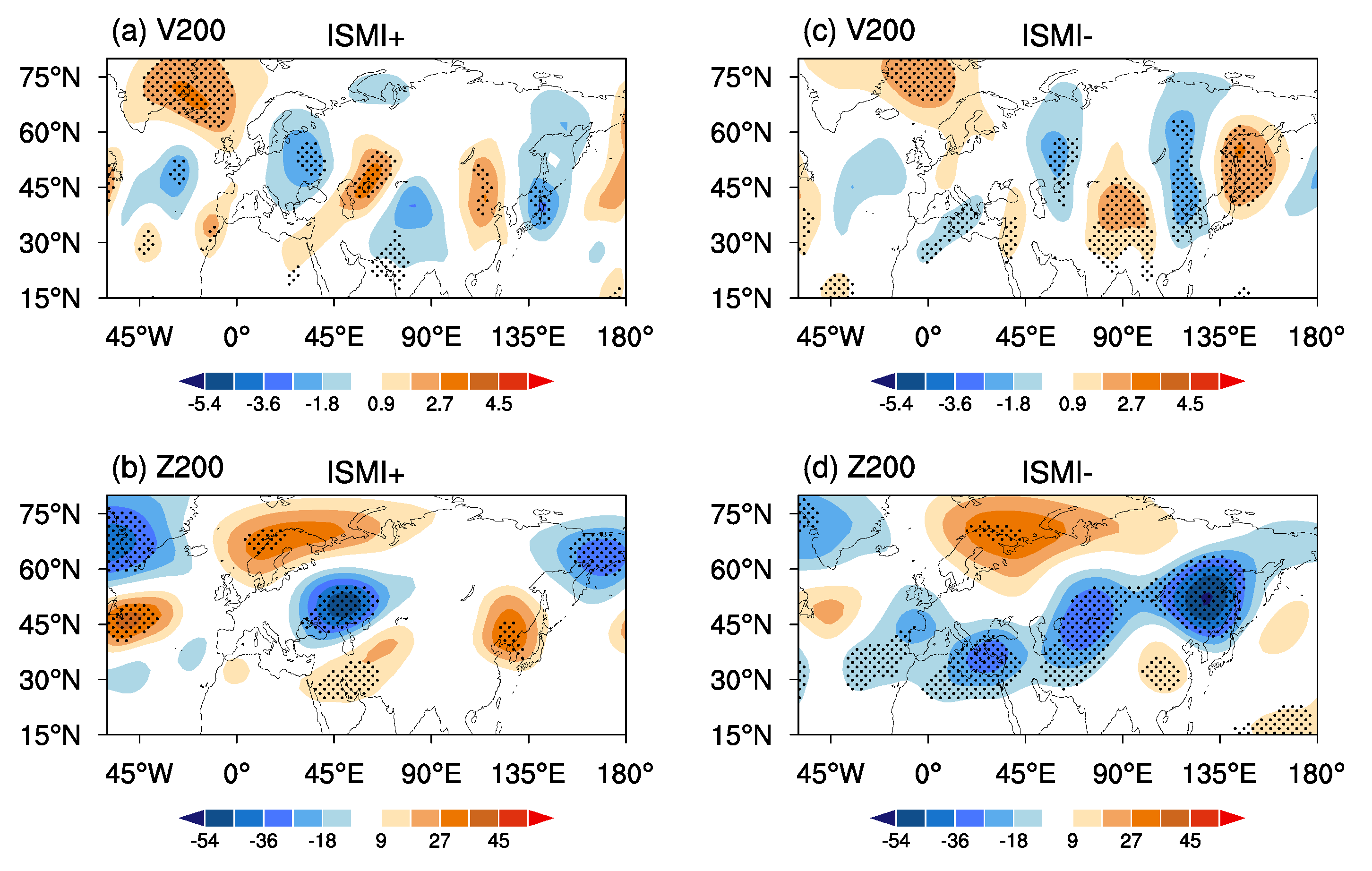
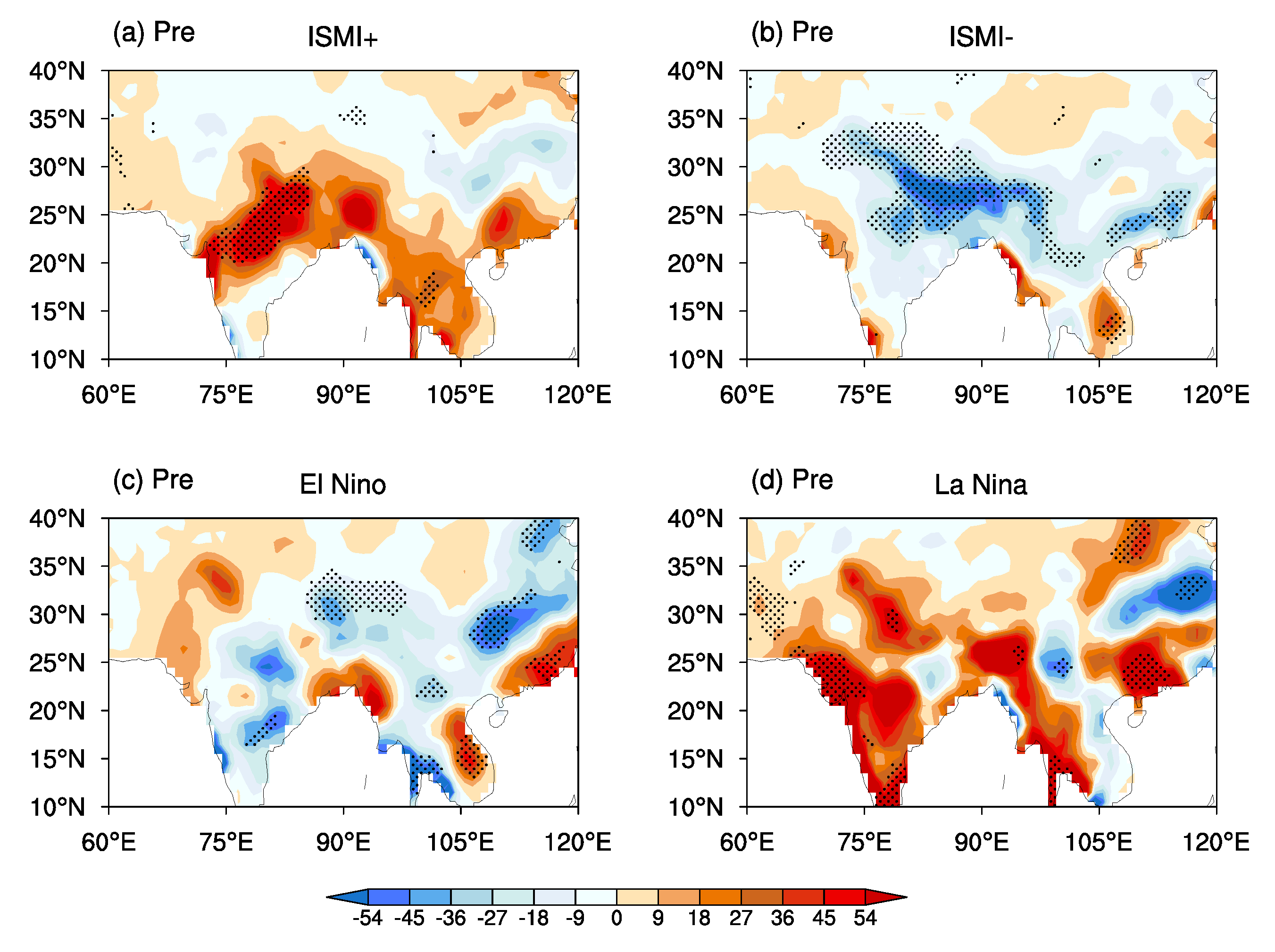
To shed light on the asymmetrical role of the ISM heating in linking the IA-SRP and IA-CGT, the V200/Z200 anomalies that regressed against the positive and negative phases of the ISMI are displayed in Figure 10. Here, the normalized ISMI with a value of above and below 0.5 standard deviations is employed in the regression analyses, aiming to clarify the asymmetrical impact of the ISM heating on the Eurasian circulations. As shown in Figure 10a,b, the V200/Z200 anomalies associated with the positive ISMI resemble those related to the positive IA-SRP/IA-CGT over Eurasia (to the south at 60 °N), corresponding to the strong linkage between the IA-SRP and IA-CGT during positive ISMI years. With respect to negative ISMI years, the associated V200/Z200 anomalies feature a wave train pattern that is similar to the negative IA-CGT over its mid/lower stream (to the east at 45 °E) and resembles the negative isolated IA-CGT (Figure 8, Figure 9 and Figure 10c,d), showing a weak connection to the circulation anomalies over the North Atlantic and Europe. These results not only confirm the essential role of the positive ISM heating in linking/triggering the IA-SRP and IA-CGT but also imply that the weak connection of the negative ISM heating to the circulation anomalies over the North Atlantic and Europe may be responsible for the difference between the IA-SRP and IA-CGT. The asymmetrical responses of the Eurasian circulations to the positive and negative ISM heating may be associated with the asymmetrical distribution of the ISM heating during its two phases. As shown in Figure 11a,b, the precipitation anomaly center is situated prominently over the northwestern ISM when the ISM heating is above normal and over the northeastern ISM when the ISM heating is below normal. The eastward shift of the ISM heating center may reduce its connection to the circulation anomalies over Europe and thereby weaken the linkage/coherence between the IA-SRP and IA-CGT, which is an interesting topic and will be examined in future work.

Figure 10.
Summer V200 (a,c) and Z200 (b,d) anomalies regressed against the (a,b) ISMI+ and (c,d) ISMI− Stippling denotes the anomalies’ significance beyond the 95% confidence level. The symbols “+” and “−” after the “ISMI” denote the year of the ISMI with values above 0.5 and below −0.5 standard deviations, respectively.
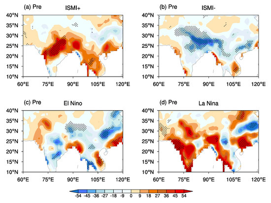
Figure 11.
Like Figure 10 but for the summer precipitation anomalies regressed against the (a) ISMI+, (b) ISMI−, (c) El Niño, and (d) La Niña. El Niño and La Niña denote the Niño3 index with values above 0.5 and below −0.5 standard deviations, respectively.
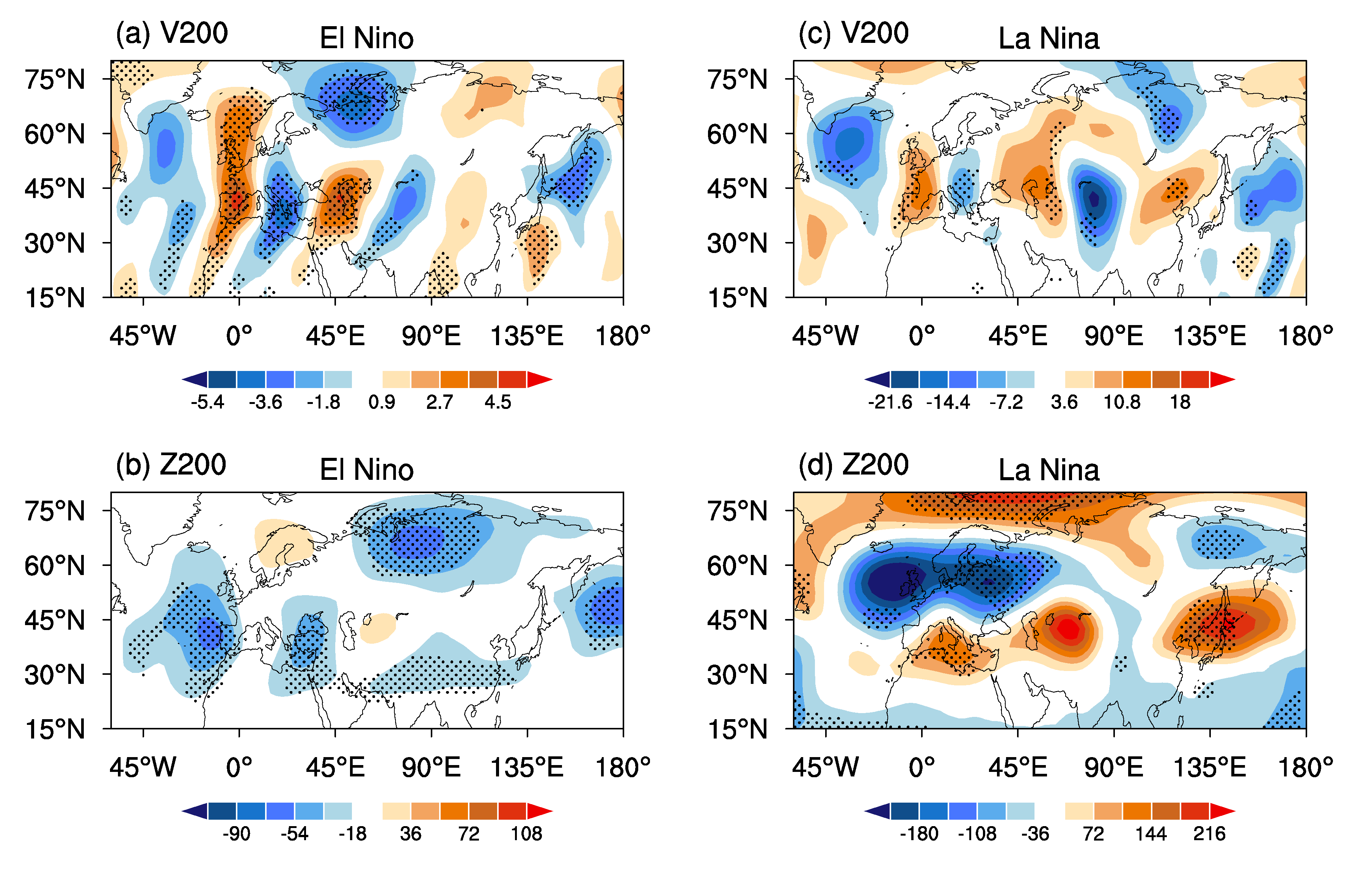
In addition to the essential role of the ISM heating, ENSO may also contribute to the linkage and difference between the IA-SRP and IA-CGT. As listed in Table 1, 18 out of the total 41 typical IA-SRP and IA-CGT cases coexist with typical ENSO cases, among which more typical ENSO cases coexist with individual IA-SRP or individual IA-CGT cases than with the co-typical cases of the IA-SRP and IA-CGT. This means that ENSO contributes largely to the difference between the two IA teleconnections. To confirm this, the V200/Z200 anomalies that regressed against the positive and negative Niño3 index (only the years in which the Niño3 index has values of above and below 0.5 standard deviations are used) are investigated. Given that ENSO and the ISM heating show a strong negative relationship (with a correlation coefficient of −0.52 between them), in particular during La Niña phases (Figure 7f and Figure 11c,d) [39], the years in which the ISMI has values of above and below 0.5 standard deviations are excluded in the regression analyses. As shown in Figure 12a,b, the V200/Z200 anomalies associated with El Niño are similar to the anomalies related to the isolated IA-SRP (Figure 3a,b). The anomalies related to the La Niña feature a similar wave train pattern to the IA-SRP/IA-CGT, albeit the anomalies are insignificant (Figure 12c,d). This means that La Niña, which often coexists with the positive ISM heating, is conducive to the linkage/coherence between the IA-SRP and IA-CGT, while El Niño contributes to the difference between them. In contrast to the ISM heating, ENSO plays a secondary role in the linkages and differences between the IA-SRP and IA-CGT.
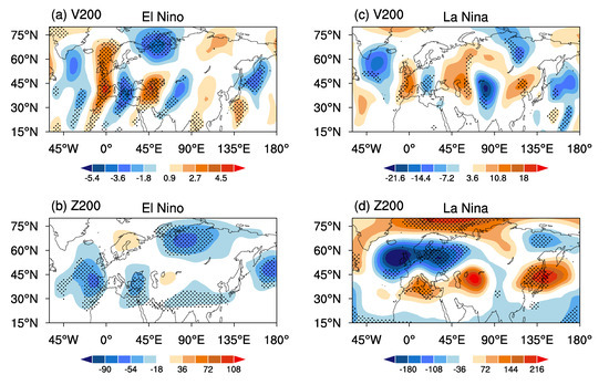
Figure 12.
Like Figure 11c,d but for the V200 (a,c) and Z200 (b,d) anomalies. Here, the years of the ISMI with values above 0.5 and below −0.5 standard deviations are excluded from the regression.
To sum up, the IA-SRP and IA-CGT reveal clear independence. The isolated IA-SRP and isolated IA-CGT mainly represent the mid-/high-latitude-related and tropics-related parts of the NH upper tropospheric circulation variations, respectively. Accordingly, the IA-SRP/IA-CGT shows a strong connection to the summer climate variations over the northern/southern part of the NH mid/high latitudes. These differences result from the asymmetrical relationship between the IA-SRP and IA-CGT during their positive and negative phases, which are mainly attributed to the asymmetrical impact of the positive and negative ISM heating on the Eurasian circulations. ENSO also contributes to the linkages and differences between the IA-SRP and IA-CGT but plays a secondary role.
5. Relationship between the SRP and CGT on the ID Timescale
5.1. Independent Parts of the ID-SRP and ID-CGT
Here, we investigate the independence between the ID-SRP and ID-CGT. In the V200 anomalies, the isolated ID-SRP retains the major wave train of the ID-SRP over the North Atlantic and Eurasia (Figure 13a). The isolated ID-CGT keeps the major structure of the ID-CGT over Korea–Japan, the North Pacific, and North America but exhibits an opposite pattern to the ID-CGT and isolated ID-SRP over Eurasia (Figure 13b). The spatial correlation coefficients of the ID-SRP and ID-CGT with their isolated counterparts are 0.73 and 0.34, respectively. In the Z200 anomalies, the isolated ID-SRP retains the major wave train pattern of the ID-SRP, especially over Eurasia, albeit its positive centers are much weaker (Figure 13c). The spatial correlation coefficient between them is about 0.61. The isolated ID-CGT reveals almost an opposite pattern to the isolated ID-SRP with positive Z200 anomalies over most parts of the NH. However, its positive centers almost overlap with the ID-CGT (Figure 13d). The spatial correlation coefficient between the ID-CGT and isolated ID-CGT is approximately 0.51. By contrast, the isolated ID-SRP keeps a larger portion of the ID-SRP/ID-CGT variations over Eurasia than the isolated ID-CGT over mid-/high-latitude Eurasia (to the north of 45 °N), while the isolated ID-CGT retains a larger portion of the ID-SRP and ID-CGT over lower-latitude Eurasia (to the south of 45 °N). These features are similar to those related to the IA-SRP and IA-CGT. In addition, it should be noted that the ID-SRP and ID-CGT feature a combined result of the isolated ID-SRP and isolated ID-CGT, while the isolated ID-SRP and isolated ID-CGT exhibit nearly an opposite structure over most parts of the NH (160 °E–360° W) except for Eurasia, with spatial correlation coefficients of −0.62 and −0.60 in the V200 and Z200 anomalies, respectively. This is why the ID-SRP and ID-CGT are stronger and more significant over Eurasia than over other parts of the NH.

Figure 13.
Like Figure 3 but for the SRP and CGT on the ID timescale.
5.2. Associations of the ID-SRP and ID-CGT with Global Climate and SST Anomalies
Figure 14 and Figure 15 illustrate the precipitation and Ts anomalies corresponding to the ID-SRP and ID-CGT as well as their independent parts. Both the ID-SRP and ID-CGT are accompanied by similar precipitation anomalies over mid-/high-latitude Eurasia, with positive anomalies over Eastern Europe and Eastern Siberia and negative anomalies over Western Europe, Northern Russia, and subtropical East Asia along the Meiyu belt (Figure 14a,b). The associated Ts anomalies also exhibit similar structures, with negative anomalies over Europe and Eastern Siberia and warm Ts over North India, West Asia, and North Russia (Figure 15a,b). The distributions of the precipitation and Ts anomalies show a good correspondence with the circulation anomalies related to the ID-SRP and ID-CGT. In addition, the ID-SRP and ID-CGT also reveal a certain connection to the precipitation/Ts anomalies over the tropics, albeit the anomalies are statistically insignificant. For example, both the ID-SRP and ID-CGT are accompanied by enhanced precipitation over the ISM and Central Pacific and reduced precipitation over the tropical Atlantic, Southeastern Indian Ocean, and Eastern Pacific (Figure 14a,b). For the Ts anomalies, significant positive anomalies are observed over the Eastern tropical Pacific and significant negative Ts anomalies are seen over the North Pacific (Figure 15a,b), which together feature a PDO-like pattern that may be associated with the positive PDO-like SST anomalies related to the two ID teleconnection patterns (see the results in Figure 16).
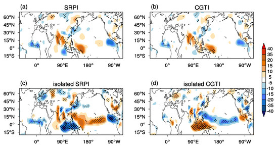
Figure 14.
Like Figure 4 but for the SRP and CGT on the ID timescale.

Figure 15.
Like Figure 5 but for the SRP and CGT on the ID timescale.
Figure 16.
Like Figure 6 but for the SRP and CGT on the ID timescale.
The precipitation/Ts anomalies associated with the isolated ID-SRP retain the major structures of those related to the ID-SRP, which have more significant and stronger anomalies over the tropics and NH extra tropics, except for West Asia (to the west of Balkashi Lake) and North India (Figure 14c and Figure 15c), where the anomalies evidently weaken. The precipitation/Ts anomalies related to the isolated ID-CGT differ largely from those related to the ID-CGT, which feature nearly opposite to those related to the isolated ID-SRP, except for the precipitation anomalies over the Eastern Indian Peninsula and the Ts anomalies over North India (Figure 14d and Figure 15d). The anti-phase precipitation/Ts anomalies related to the isolated ID-SRP and isolated ID-CGT are responsible for the statistically insignificant precipitation/Ts anomalies associated with the ID-SRP and ID-CGT over most parts of the tropics and NH extra tropics.
Previous studies have shown that the ID-SRP and ID-CGT are modulated by the ID SST anomalies over the North Atlantic and North Pacific [25,27,29]. As shown in Figure 16, the ID-SRP and ID-CGT tend to occur during the positive phase of the PDO and the negative phase of the AMO, particularly during summer. The correlation coefficients of the ID-SRPI/ID-CGTI with the summer PDO and AMO indices on the ID timescale are 0.65/0.56 and −0.54/−0.45, respectively. The confidence levels for the four correlation coefficients are 94%, 88%, 89%, and 81%, respectively. When removing the signal of each counterpart, the PDO-like and AMO-like SST anomalies remain during summer in relation to the isolated ID-SRP but disappear in relation to the ID-CGT. From this aspect, the PDO and AMO are more likely the driving factors of the ID-SRP. This is to some extent consistent with previous studies on the linkages of the PDO and AMO to the ID circumglobal wave train over the NH [27,40].
The independence of the ID-SRP and ID-CGT and their associations with global climate and SST anomalies are not as well organized as their IA counterparts, which makes it hard to clarify which factors are responsible for their differences. This is due to the high spatial and temporal correlations (with values of 0.97 and 0.88, respectively) between the ID-SRP and ID-CGT.
6. Conclusions and Discussion
The SRP and CGT are two well-known teleconnection patterns along the Eurasian westerly jet during boreal summer. Due to their highly spatial-temporal similarity, the SRP and CGT are often regarded as one teleconnection pattern. Given their different definitions as well as distinct features on the IA and ID timescales, the present work investigates the linkages and differences between the SRP and CGT on the IA and ID timescales, respectively, aiming to provide a comprehensive view of the SRP–CGT relationship. The main results are summarized as follows.
On the IA timescale, the SRP and CGT reveal high spatial-temporal similarity, and both clearly exhibit a circumglobal wave train over the NH mid-latitudes, with significant and strong active centers over Eurasia. For their independent parts, the isolated IA-SRP retains the IA-SRP structure and shows a strong impact on the summer climate over the northern part of the mid-/high-latitude NH (to the north at about 45 °N). The isolated IA-CGT reserves the major structure of the IA-CGT and has a strong impact on the summer climate over the southern part of the NH mid-latitudes (to the south at about 45 °N). The isolated IA-CGT shows a stronger connection to the ISM heating and ENSO than the isolated IA-SRP. This makes the IA-CGT more like a tropical forcing-driven atmospheric mode, while the IA-SRP is more like an internal atmospheric mode, although it can be modulated by mid-latitude disturbances, ISM heating, and ENSO. From this aspect, the IA-SRP and IA-CGT may largely represent the mid-/high-latitude-related and tropics-related parts of the NH upper tropospheric circulation variations, respectively.
The linkages and differences between the IA-SRP and IA-CGT correspond to their strong and weak coherence during their positive and negative phases, respectively, which are mainly attributed to the asymmetrical impact of the ISM heating on the two teleconnection patterns. Positive ISM heating favors a linkage/coherence between the IA-SRP and IA-CGT by triggering a positive IA-SRP-like/IA-CGT-like wave train pattern over the area of the North Atlantic, Europe, and Asia. Negative ISM heating shows a weak impact on the European circulations and often excites a wave train pattern over the area from North Africa to East Asia, which features a negative IA-CGT-like pattern, contributing to the difference between the IA-SRP and IA-CGT. ENSO plays a secondary role in the linkages and differences between the IA-SRP and IA-CGT, with El Niño contributing to their differences and La Niña to their linkages.
On the ID timescale, both the ID-SRP and ID-CGT feature a two-wave train structure over Eurasia, with one weak wave train and another prominent wave train located to the south and north of 45 °N, respectively. They bear a high spatial-temporal similarity, with spatial and temporal correlation coefficients of 0.97 and 0.88, respectively. These features make the ID-SRP and ID-CGT more like the same teleconnection pattern, in particular over Eurasia. In addition, the ID-SRP shows a strong connection to the PDO and AMO. This means that the PDO and AMO are more likely the driving factors of the ID-SRP.
It should be noted that the present findings regarding the SRP–CGT relationship on the IA and ID timescales are different from those of Zhou et al. [31], who regarded the CGT as a section of the SRP. This discrepancy is due to the fact that they overlooked the distinction between the SRP and CGT on the IA and ID timescales, as well as the impact of the linear trend on their ID variations. More importantly, the clear differences between the IA-SRP and IA-CGT in their structures, associations with Eurasian summer climate, the ISM heating, and ENSO imply that the IA-SRP and IA-CGT should not be simply regarded as the same teleconnection pattern, and they actually capture different portions of the NH upper tropospheric circulation variations. Also, these differences make the prediction of the SRP or CGT variations much more difficult, as argued by Kosaka et al. [6], who stated that the contemporary initialized coupled prediction systems cannot achieve a reliable prediction of the SRP phase at monthly to seasonal lead times. The present findings on the linkages and differences between the SRP and CGT, in particular on the IA timescale, are beneficial to understanding the variability and prediction of the SRP and CGT, which have important implications for seasonal climate prediction over the NH extra-tropics.
Supplementary Materials
The following supporting information can be downloaded at https://www.mdpi.com/article/10.3390/atmos14111626/s1, Figure S1. Summer (a) Z200 regressed against the normalized principal component (b) of the second EOF of the Z200 over the NH (to the north of 20 °N). Figure S2. Summer (a) V200 and (b) Z200 anomalies regressed against the undetrended SRPI (shading) and undetrended CGTI (contour) on the IA timescale with the linear trend of the data and indices reserved. (c,d) Same as (a,b) but on the ID timescale. The horizontal/vertical lines in (a–d) display the V200 and Z200 anomalies regressed against the undetrended SRPI/CGTI on the IA and ID timescales’ significance beyond the 95% confidence level. The units for the V200 and Z200 are ms−1 and gpm, respectively. Table S1. Description of the five SRP indices, their explanation percentage, and correlation with the SRP index defined by Yasui and Watanabe (2010) used in the present study on the total, IA, and ID timescales. The bold and asterisked correlation coefficients are significant beyond 99% and 95% confidence levels, respectively. Table S2. Variance explanation percentages of the detrended (regular number) and undetrended (bold number) IA and ID components of the SRP and CGT to their total variances. Table S3. Correlation coefficients between the total, IA, and ID components of the SRPI and CGTI. The regular and bold numbers denote the correlation coefficients between the IA/ID components of the SRPI and CGTI without and with the linear trend, respectively. The asterisk represents the correlation coefficient significance beyond the 95% confidence level.
Funding
This study is jointly supported by the National Natural Science Foundation of China (grant Nos. 41605058 and 41831175), the Joint Open Project of the Key Laboratory of Meteorological Disaster, Ministry of Education, and the Collaborative Innovation Center on Forecast and the Evaluation of Meteorological Disasters, NUIST (KLME202104).
Data Availability Statement
The atmospheric circulation and surface air temperature is provided by the National Centers for Environmental Prediction and Atmospheric Research (https://downloads.psl.noaa.gov/Datasets/ncep.reanalysis/Monthlies/). The precipitation data is provided by the National Oceanic and Atmospheric Administration’s precipitation reconstruction (PREC) dataset (https://downloads.psl.noaa.gov/Datasets/prec/). The global SST from the Hadley Centre can be download from https://hadleyserver.metoffice.gov.uk/hadsst2/data/download.html. The PDO index and AMO index were downloaded from https://www.esrl.noaa.gov/psd/data/correlation/pdo.data and https://www.esrl.noaa.gov/psd/data/correlation/amon.us.data, respectively.
Acknowledgments
We thank the three anonymous reviewers for their constructive comments that led to the improvements of the manuscript. This study is jointly supported by the National Natural Science Foundation of China (grant Nos. 41605058 and 41831175), the Joint Open Project of the Key Laboratory of Meteorological Disaster, Ministry of Education, and the Collaborative Innovation Center on Forecast and the Evaluation of Meteorological Disasters, NUIST (KLME202104).
Conflicts of Interest
The authors declare no conflict of interest.
References
- Lu, R.Y.; Oh, J.H.; Kim, B.J. A teleconnection pattern in upper-level meridional wind over the North African and Eurasian continent in summer. Tellus Ser. A Dyn. Meteorol. Oceanogr. 2002, 54, 44–55. [Google Scholar] [CrossRef]
- Enomoto, T. Interannual variability of the Bonin high as- sociated with the propagation of Rossby waves along the Asian jet. J. Meteor. Soc. Jpn. 2004, 82, 1019–1034. [Google Scholar] [CrossRef]
- Ding, Q.; Wang, B. Circumglobal teleconnection in the Northern Hemisphere summer. J. Clim. 2005, 18, 3483–3505. [Google Scholar] [CrossRef]
- Yasui, S.; Watanabe, M. Forcing processes of the summertime circumglobal teleconnection pattern in a dry AGCM. J. Clim. 2010, 23, 2093–2114. [Google Scholar] [CrossRef]
- Kosaka, Y.; Nakamura, H. Mechanisms of meridional teleconnection observed between a summer monsoon system and a subtropical anticyclone. Part I: The Pacific-Japan pattern. J. Clim. 2010, 23, 5085–5108. [Google Scholar] [CrossRef]
- Kosaka, Y.; Xie, S.P.; Nakamura, H. Dynamics of interannual variability in summer precipitation over East Asia. J. Clim. 2011, 24, 5435–5453. [Google Scholar] [CrossRef]
- Huang, G.; Liu, Y.; Ronghui, H. The Interannual Variability of Summer Rainfall in the Arid and Semiarid Regions of Northern China and Its Association with the Northern Hemisphere Circumglobal Teleconnection.pdf. Adv. Atmos. Sci. 2011, 28, 257–268. [Google Scholar] [CrossRef]
- Huang, R.H.; Liu, Y.; Feng, T. Interdecadal change of summer precipitation over Eastern China around the late-1990s and associated circulation anomalies, internal dynamical causes. Chin. Sci. Bull. 2013, 58, 1339–1349. [Google Scholar] [CrossRef]
- Hong, X.; Lu, R.; Li, S. Amplified summer warming in Europe-West Asia and Northeast Asia after the mid-1990s. Environ. Res. Lett. 2017, 12, 094007. [Google Scholar] [CrossRef]
- Gong, Z.; Feng, G.; Dogar, M.M.; Huang, G. The possible physical mechanism for the EAP–SR co-action. Clim. Dyn. 2018, 51, 1499–1516. [Google Scholar] [CrossRef]
- Liu, Y.; Huang, R. Linkages between the South and East Asian Monsoon water vapor transport during boreal summer. J. Clim. 2019, 32, 4509–4524. [Google Scholar] [CrossRef]
- Enomoto, T.; Hoskins, B.J.; Matsuda, Y. The formation mechanism of the Bonin high in August. Q. J. R. Meteorol. Soc. 2003, 129, 157–178. [Google Scholar] [CrossRef]
- Sato, N.; Takahashi, M. Dynamical processes related to the appearance of quasi-stationary waves on the subtropical jet in the midsummer northern hemisphere. J. Clim. 2006, 19, 1531–1544. [Google Scholar] [CrossRef]
- Kosaka, Y.; Nakamura, H.; Watanabe, M.; Kimoto, M. Analysis on the Dynamics of a Wave-like Teleconnection Pattern along the Summertime Asian Jet Based on a Reanalysis Dataset and Climate Model Simulations. J. Meteorol. Soc. Jpn. 2009, 87, 561–580. [Google Scholar] [CrossRef]
- Chen, G.; Huang, R. Excitation mechanisms of the teleconnection patterns affecting the July precipitation in Northwest China. J. Clim. 2012, 25, 7834–7851. [Google Scholar] [CrossRef]
- Chen, G.; Huang, R.; Zhou, L. Baroclinic Instability of the Silk Road Pattern Induced by Thermal Damping. J. Atmos. Sci. 2013, 70, 2875–2893. [Google Scholar] [CrossRef]
- Wu, R. A mid-latitude Asian circulation anomaly pattern in boreal summer and its connection with the Indian and East Asian summer monsoons. Int. J. Climatol. 2002, 22, 1879–1895. [Google Scholar] [CrossRef]
- Ding, Q.; Wang, B.; Wallace, J.M.; Branstator, G. Tropical-extratropical teleconnections in boreal summer: Observed interannual variability. J. Clim. 2011, 24, 1878–1896. [Google Scholar] [CrossRef]
- Lin, Z.; Lu, R. Impact of summer rainfall over southern-central Europe on circumglobal teleconnection. Atmos. Sci. Lett. 2016, 17, 258–262. [Google Scholar] [CrossRef]
- Lin, Z.; Lu, R.; Wu, R. Weakened impact of the Indian early summer monsoon on north China rainfall around the late 1970s: Role of basic-state change. J. Clim. 2017, 30, 7991–8005. [Google Scholar] [CrossRef]
- Hong, X.W.; Lu, R.Y.; Chen, S.F.; Li, S.L. The Relationship between the North Atlantic Oscillation and the Silk Road Pattern in Summer. J. Clim. 2022, 35, 3091–3102. [Google Scholar] [CrossRef]
- Liu, Y.; Zhou, W.; Qu, X.; Wu, R.G. An Interdecadal Change of the Boreal Summer Silk Road Pattern around the Late 1990s. J. Clim. 2020, 33, 7083–7100. [Google Scholar] [CrossRef]
- Wu, R.; Wang, B. A contrast of the East Asian summer monsoon-ENSO relationship between 1962-77 and 1978-93. J. Clim. 2002, 15, 3266–3279. [Google Scholar] [CrossRef]
- Wang, H.; Wang, B.; Huang, F.; Ding, Q.; Lee, J.Y. Interdecadal change of the boreal summer circumglobal teleconnection (1958–2010). Geophys. Res. Lett. 2012, 39, L12704. [Google Scholar] [CrossRef]
- Wang, L.; Xu, P.; Chen, W.; Liu, Y. Interdecadal variations of the Silk Road pattern. J. Clim. 2017, 30, 9915–9932. [Google Scholar] [CrossRef]
- Hong, X.-W.; Xue, S.-H.; Lu, R.-Y.; Liu, Y.-Y. Comparison between the interannual and decadal components of the Silk Road pattern. Atmos. Ocean. Sci. Lett. 2018, 11, 270–274. [Google Scholar] [CrossRef]
- Stephan, C.C.; Klingaman, N.P.; Turner, A.G. A mechanism for the interdecadal variability of the Silk Road Pattern. J. Clim. 2019, 32, 717–736. [Google Scholar] [CrossRef]
- Wang, H.; Huang, F.; Yang, Y.X. Reanalysis on the interdecadal variability of the circumglobal teleconnection. J. Ocean Univ. China 2013, 43, 1–8. (In Chinese) [Google Scholar]
- Wu, B.; Lin, J.; Zhou, T. Interdecadal circumglobal teleconnection pattern during boreal summer. Atmos. Sci. Lett. 2016, 17, 446–452. [Google Scholar] [CrossRef]
- Xu, P.; Wang, L.; Chen, W. The British–Baikal Corridor: A Teleconnection Pattern along the Summertime Polar Front Jet over Eurasia. J. Clim. 2019, 32, 877–896. [Google Scholar] [CrossRef]
- Zhou, F.; Zhang, R.; Han, J. Relationship between the Circumglobal Teleconnection and Silk Road Pattern over Eurasian continent. Sci. Bull. 2019, 64, 374–376. [Google Scholar] [CrossRef]
- Kalnay, E.; Kanamitsu, M.; Kistler, R.; Collins, W.; Deaven, D.; Gandin, L. The NCEP/NCAR 40-Year Reanalysis Project. Bull. Am. Meteorol. Soc. 1996, 77, 437–472. [Google Scholar] [CrossRef]
- Chen, M.; Xie, P.; Janowiak, J.E.; Arkin, P.A. Global Land Precipitation: A 50-yr Monthly Analysis Based on Gauge Observations. J. Hydrometeor. 2002, 3, 249–266. [Google Scholar] [CrossRef]
- Rayner, N.A. Global analyses of sea surface temperature, sea ice, and night marine air temperature since the late nineteenth century. J. Geophys. Res. 2003, 108, 4407. [Google Scholar] [CrossRef]
- Duchon, C.E. Lanczos Filtering in One and Two Dimensions. J. Appl. Meteor. 1979, 18, 1016–1022. [Google Scholar] [CrossRef]
- Metz, W. Optimal Relationship of Large-Scale Flow Patterns and the Barotropic Feedback Due to High-Frequency Eddies. J. Atmos. Sci. 1991, 48, 1141–1159. [Google Scholar] [CrossRef]
- Trenberth, K.E.; Branstator, G.W.; Karoly, D.; Kumar, A.; Lau, N.; Ropelewski, C. Progress during TOGA in understanding and modeling global teleconnections associated with tropical sea surface temperatures. J. Geophys. Res. 1998, 103, 14291–14324. [Google Scholar] [CrossRef]
- Seager, R.; Harnik, N.; Kushnir, Y.; Robinson, W.; Miller, J.A. Mechanisms of hemispherically symmetric climate variability. J. Clim. 2003, 16, 2960–2978. [Google Scholar] [CrossRef]
- Kumar, K.K.; Rajagopalan, B.; Hoerling, M.; Bates, G.; Cane, M. Unraveling the Mystery of Indian Monsoon Failure During El Niño. Science 2006, 314, 115–119. [Google Scholar] [CrossRef]
- Zhu, Y.; Wang, H.; Ma, J.; Wang, T.; Sun, J. Contribution of the phase transition of Pacific Decadal Oscillation to the late 1990s’ shift in East China summer rainfall. J. Geophys. Res. 2015, 120, 8817–8827. [Google Scholar] [CrossRef]

Disclaimer/Publisher’s Note: The statements, opinions and data contained in all publications are solely those of the individual author(s) and contributor(s) and not of MDPI and/or the editor(s). MDPI and/or the editor(s) disclaim responsibility for any injury to people or property resulting from any ideas, methods, instructions or products referred to in the content. |
© 2023 by the author. Licensee MDPI, Basel, Switzerland. This article is an open access article distributed under the terms and conditions of the Creative Commons Attribution (CC BY) license (https://creativecommons.org/licenses/by/4.0/).