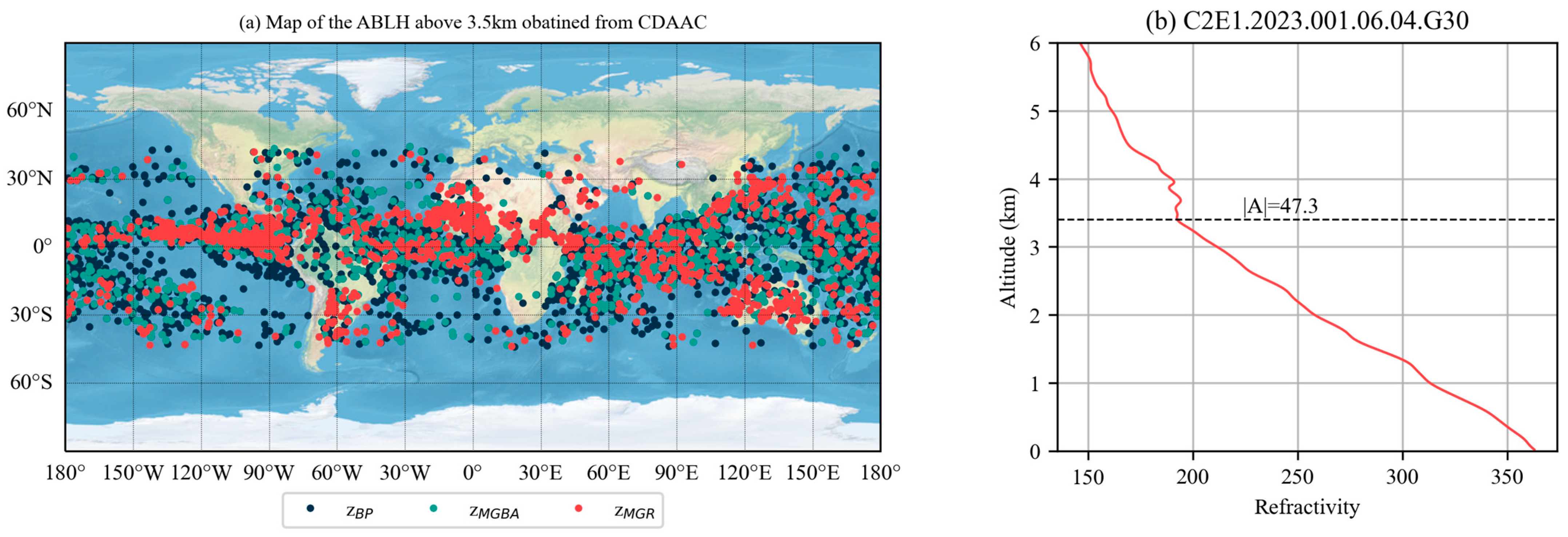
3.1. Initial Analysis
CDAAC provides ABLHs calculated using the MG method with bending angle, the MG method with refractivity, and the BP methods [
23]. Before proceeding with the comparison of the five different methods, we analyze the characteristics of the
,
, and
, calculated by CDAAC. As shown in
Figure 1a, some of the ABLHs obtained from the COSMIC-2 data penetrating the below 0.5 km, particularly in the oceanic region, surpass the threshold of 3.5 km. Additionally,
Figure 1b illustrates that the
do not align with the criteria of |A| > 50 km
−1 proposed by Guo et al. (2011) [
8]. Hence, these values obtained from CDAAC are considered to be raw and have not been filtered according to the specific criteria, making them unreliable and inconsistent with actual atmospheric conditions. Therefore, instead of using the ABLH results provided by CDAAC for the comparative study, we determined the values of
,
, and
using the abovementioned formulae and conducted outlier screening based on the criteria described in
Section 2.3.
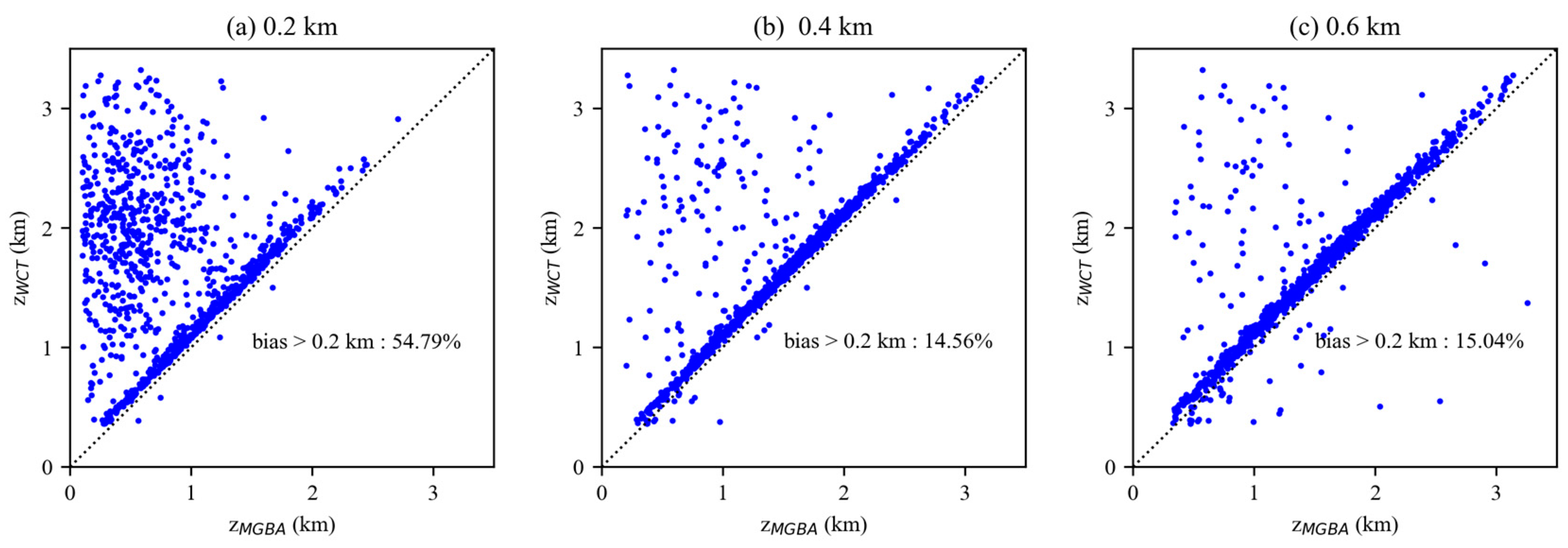
Based on the experiment conducted by Ratnam et al. (2010) [
14], different dilations, ranging from 0.2 km to 0.6 km in intervals of 0.2 km, were selected. To make the dilation more representative of most GNSS-RO profiles, a single GNSS-RO profile was not chosen; instead, all the data on 29 February 2022 were selected to compare the effects of different dilations. Furthermore, it will be compared to the ABLHs calculated using other methods with GNSS-RO profiles. To avoid similarities introduced by the same refractivity profiles, bending angle profiles were used instead. Additionally, considering that the MG method was applied to the determination of AHLH with RO data earlier (than DPMF method) and has received more validation, the MGBA method will be employed.
In
Figure 2, the proportions of biases > 0.2 km between
and
are 54.79%, 14.56%, and 15.04%, corresponding to dilations of 0.2 km, 0.4 km, and 0.6 km, respectively. Therefore, the optimal dilation value should be set to 0.4 km.
3.2. Comparison of the RO- and RAOB-Derived ABLHs
To minimize the potential impact of landform and physiognomy on the comparison, the comparison was initiated using data in islands and coastal regions. Therefore, 61 globally distributed RAOB stations (
Figure 3) on islands or along coastlines were selected to collocate with the data from GNSS-RO. Additionally, due to GNSS-RO data originating from different RO missions, it was necessary to analyze the COSMIC-2 and Spire data independently to prevent any potential systematic errors.
In this study, using the ABLHs (
) derived from RAOB atmospheric profiles as a reference, we evaluated the performances of the ABLHs (
), including
,
,
,
, and
determined from the COSMIC-2 data using five different methods. As shown in
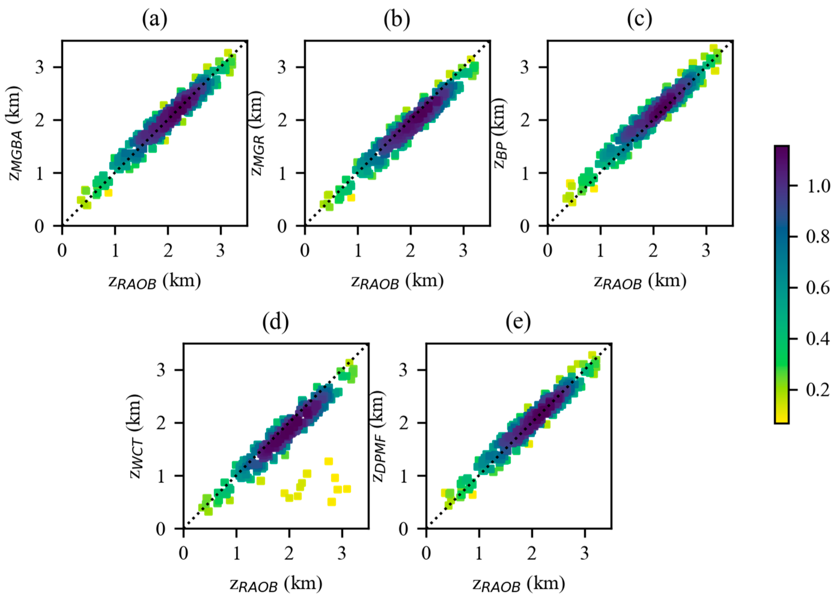
Figure 4, the comparison results indicate a good agreement between the
and
over oceans. The colorbar represents a Gaussian kernel density estimation.
Table 1 presents the correlation coefficients between the
and
derived from COSMIC-2, as well as the biases and root-mean-square error (RMSE) of the
derived from COSMIC-2 compared to the
. Higher positive correlation coefficients for
(0.967),
(0.968),
(0.966),
(0.969), and
(0.967) indicate closer matching between
and
. The differences in the correlation coefficients between
and
were not significant. In terms of bias and RMSE,
agreed closely with
, and were, in descending order:
,
,
,
, and
.
exhibited the smallest bias (0.023 km) with an RMSE of 0.173 km and the best agreement with
, while
showed the most noticeable (positive) bias of 0.100 km, with an RMSE of 0.2 km.
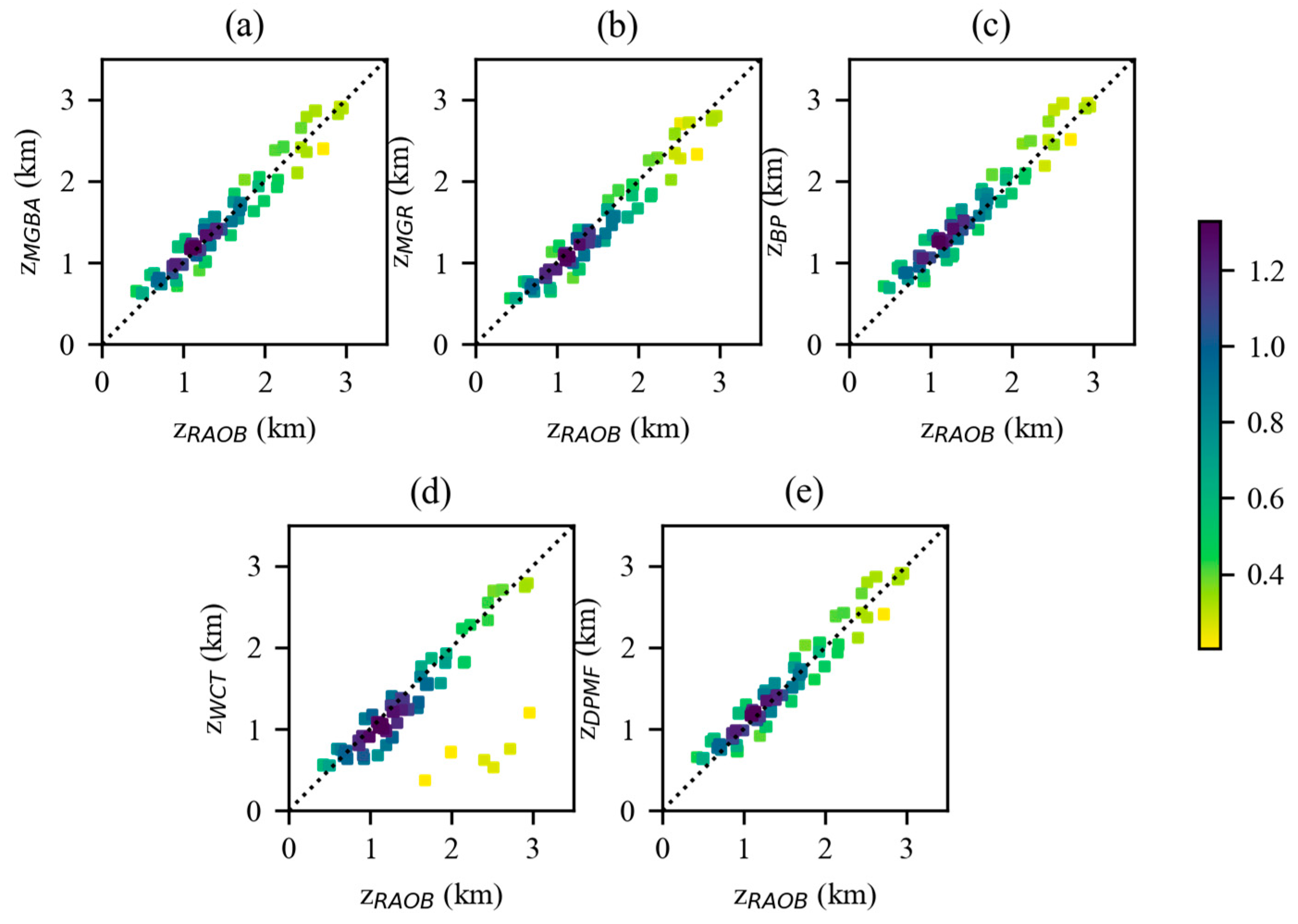
Figure 5 shows the scatter density plots of the
and
over oceans determined from the Spire data, suggesting a satisfactory agreement between the
and
, except for the
determined using the WCT method, which had an obvious negative bias compared to the
. Specifically, some
values were significantly smaller than the values of corresponding
, with biases of more than ~1.2 km. In
Table 2, the correlation coefficient between the
calculated from Spire and
is 0.686. Compared to the correlation between the
derived from COSMIC-2 and
(0.969), the correlation weakened significantly. Moreover, the bias and RMSE were relatively large. In terms of bias and RMSE,
agreed closely with
, and were, in descending order:
,
,
,
, and
. The bias and RMSE for
remained the smallest compared to those from COMSIC-2, showing the closest agreement with
.
Compared to RAOB stations on islands and near coastal regions, there are more RAOB stations on land, and the ABLH over land shows a greater variability than that over the ocean. However, inland RAOB stations are more affected by landform and physiognomy. Therefore, we only considered stations with altitudes below 0.5 km, located deep inland at least 300 km away from the coast, to avoid the influence of coastal and oceanic areas. The distribution of inland RAOB stations is shown in
Figure 6.
Figure 7 displays the scatter density plots of the
and
calculated from the COSMIC-2 data for inland regions.
Table 3 shows the statistical analysis results of the
and
inland from the COSMIC-2 data. Combining the statistical results from
Table 3, the main findings and the results from the
over oceans for Spire were similar. The number of RO profiles over oceans was relatively limited, which may explain why smaller
values were not found in the COSMIC-2 oceanic data. This suggests that the cause of the significantly lower
compared to
was likely inherent to the WCT method itself, rather than the Spire RO data.
In
Figure 8, the scatter density plots of the
and
inland calculated from the Spire data are shown.
Table 4 presents the statistical analysis results of the
and
from the Spire data for inland regions. In
Figure 8, the ABLHs calculated by Spire in the range from 1 to 1.5 km are denser compared to COSMIC-2. There is a greater quantity of data in the range from 1 to 1.5 km, in contrast to the inland ABLHs obtained from COSMIC-2. This was mainly because COSMIC-2 is concentrated in mid-latitude regions, whereas Spire offers global coverage. The ABLH in mid-latitude regions was higher compared to that in high-latitude regions [
24].
Based on the statistical data presented in
Table 1,
Table 2,
Table 3 and
Table 4, it can be observed that there were no significant differences in the biases and RMSE of the
from Spire and COSMIC-2 compared to the
, except in the case of the WCT method. As multiple reports and studies have already compared and evaluated data from both COSMIC-2 and Spire, and considering the high similarity in the bending angle and refractivity accuracy [
25,
26], we will not discuss these aspects separately in the following content.
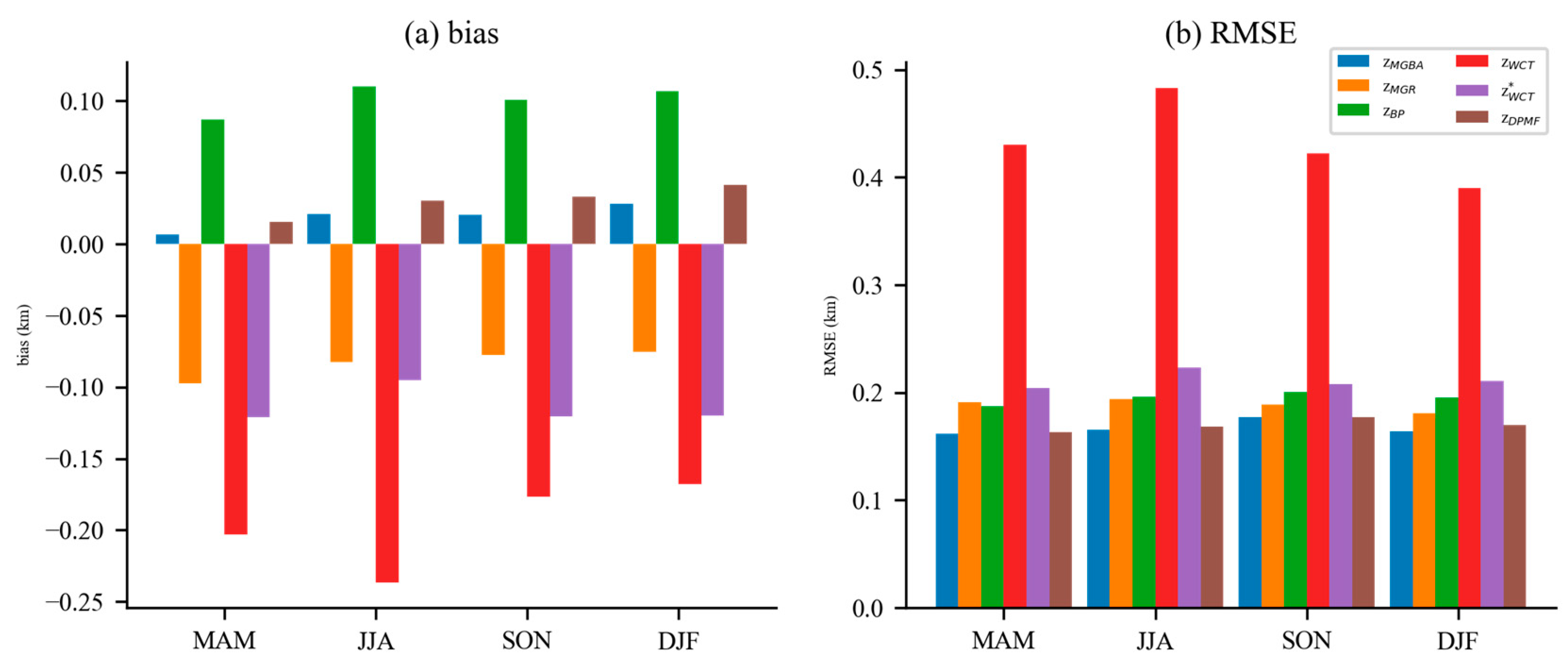
Figure 9 illustrates the biases and RMSE of the
over oceans in the Northern Hemisphere using the five different methods across four seasons (MAM: from March to May, JJA: from June to August, SON: from September to November, and DJF: from December to February). Specially,
represents the
without a bias of more than 1.2 km with
. In all four seasons,
consistently had the largest bias and RMSE among the five methods. Notably, the biases of
and
exhibited seasonal variability, with the highest biases being observed during JJA and the lowest during DJF. Conversely, the RMSE values for the
,
,
, and
did not exhibit pronounced seasonal variations. The biases of
were smaller than those of
, which was due to the removal of data with biases exceeding 1.2 km. The RMSE of
was then relatively close to that of other
. However, the biases and RMSE of
still showed some seasonal characteristics, possibly because larger biases were not completely removed, and the lower number of collocated RO profiles over oceans made it difficult to effectively reduce errors through averaging. It is possible that this was caused by the lower quality of the GNSS-RO refractivity profiles near the Earth’s surface. Near the surface, super-refraction and signal tracking errors are more likely to occur, leading to negative biases in refractivity [
27,
28,
29]. Environments with high humidity are more prone to inducing super-refraction [
30]. As a result, the bias and RMSE of
are more likely to exhibit seasonal variations. Further analysis will be conducted in
Section 3.4.
In
Figure 10, the deviation and RMSE between
and
within the Northern Hemisphere’s inland regions are presented. It can be observed that the
in inland areas did not exhibit significant seasonal variations, due to a larger number of profiles, which helped to reduce errors through averaging. From
Table 1,
Table 2,
Table 3 and
Table 4 and
Figure 9 and
Figure 10, it is evident that
performed the best and was closest to the RAOB measurements.
3.3. Comparison of the RO-Derived ABLHs
The comparisons between the ABLHs derived from the RO data and the RAOB in
Section 3.1 are restricted only to the vicinity of RAOB stations. To further compare the ALBHs derived from RO data on a large spatial scale, we conducted a comprehensive investigation of MBLHs globally. Based on the above analysis,
exhibited the smallest error. Therefore, we used
as a reference value to analyze other
.
Figure 11 shows the annual-averaged differences of
,
,
, and
w.r.t.
over oceans for the period from 1 March 2022 to 28 February 2023 in a given latitude–longitude bin with a resolution of 1° × 1°. In ascending order w.r.t. the differences from
, they were
,
,
, and
. Specifically, the differences for
and
were negative, while those for
and
were positive. The
values were relatively lower than the other
values. This was because
exhibited a significant negative bias, as presented in
Section 3.2.
The boxplot in
Figure 12 graphically shows the distribution of the MBLHs determined by the five methods from 1 March 2022 to 28 February 2023. The box extends from the first quartile (Q1) to the third quartile (Q3), and the yellow line indicates the median value. More detailed information on the median, Q1, and Q3 values for the MBLHs obtained using each method can be found in
Table 5. Among the five methods, the distributions of
and
showed a better agreement with each other than with the others, with a median value of about 1.6 km. Compared to
and
, the median value of
(1.820) was relatively high, while the median value of
(1.598) wazs relatively low. The values of
, on the other hand, were significantly lower than those of the other methods, which is consistent with the results presented in
Section 3.2.
3.4. Analysis on the Biases of the RO-Derived ABLHs
The experimental analysis mentioned above involved the outlier screening of using the five methods. was consistently lower than the ABLHs obtained using other methods. This discrepancy may be attributed to the sensitivity of the WCT method to refractivity mutations near the Earth’s surface. In this case, outlier screening was removed to facilitate the comparison of the differences among the five methods, especially the WCT method.
Compared to
Figure 12 and
Table 5, as shown in
Figure 13 and
Table 6, the median values of the MBLH calculated using the five methods decreased. This was due to the outlier screening process, which removed data with larger differences. MBLH values near the Earth’s surface are more numerous and contain more errors, making them more likely to be removed. Without outlier screening, the number of smaller values for
would increase noticeably, followed by
. In contrast, the boxplots of the other three methods show relatively small variations after the outlier screening (as seen in
Figure 12). The DPMF and WCT methods attempt to utilize data near the lower troposphere more extensively than the other three methods. However, the RO profiles near the lower troposphere are associated with larger errors and significant variations, resulting in the unreliability of the
and
.
As shown in
Figure 14, a GNSS-RO event profile of bending angle (red line) and refractivity (blue line) was selected to further analyze the biases of the RO-derived ABLHs. The WCT and DPMF methods detected strong variations in the profiles near the Earth’s surface and considered them as ABLHs. Through comparison to
, it became evident that these pronounced fluctuations were more likely caused by errors. Using other three
as auxiliary information, the heights of the minimum points closest to the values of other three
were considered as the ABLHs obtained using WCT and DPMF (corresponding to
and
).
Basing their values on the other three , the occurrence of significantly lower values in the case of the and was considered as an outlier. We conducted a statistical analysis on the occurrence of lower values for and from 1 March 2022 to 28 February 2023, and found that the probabilities were 10.50% and 4.24%, respectively.


 ,
, 


