Article

Identification of Airborne Particle Types and Sources at a California School Using Electron Microscopy

1
Environmental Health Laboratory Branch, California Department of Public Health, Richmond, CA 94804, USA
2
Center for Environmental Research and Community Health, School of Public Health, University of California, Berkeley, CA 94704, USA
3
Office of Environmental Health Hazard Assessment, California Environmental Protection Agency, Oakland, CA 94612, USA
4
Department of Civil and Environmental Engineering, University of California, Berkeley, CA 94720, USA
5
Division of Environmental Health Sciences, School of Public Health, University of California, Berkeley, CA 94704, USA
6
Department of Public Health, University of California, Merced, CA 95343, USA
7
Environmental Health Investigations Branch, California Department of Public Health, Richmond, CA 94804, USA
*
Author to whom correspondence should be addressed.
Atmosphere 2023, 14(11), 1702; https://doi.org/10.3390/atmos14111702
Submission received: 7 October 2023 / Revised: 10 November 2023 / Accepted: 16 November 2023 / Published: 20 November 2023
(This article belongs to the Special Issue Chemical and Morphological Characterization of Atmospheric Aerosols)

Abstract

:
We conducted a pilot study to investigate air quality indoors in two classrooms and outdoors on the school grounds in a California community with historically high PM2.5 (fine particulate matter, diameter < 2.5 μm). We used computer-controlled scanning electron microscopy of passive samples to identify major PM types, which were used to help interpret continuous PM2.5 and black carbon sensor data. The five major PM types were sodium salt particles with sulfur, calcium, or chlorine; aluminosilicate dusts; carbonaceous combustion agglomerates; biogenic particles; and metal-rich particles. Based on morphological evidence of water droplets, the salt particles are hypothesized to be secondary aerosols formed via the reaction of sodium chloride fog droplets with sulfur from regional sources. The carbonaceous agglomerates had unusual morphologies consistent with low-temperature combustion and smoke from open-burning activities observed nearby. The passive PM sampler and continuous sensor results indicated lower concentrations in the classroom equipped with an air cleaner. Passive samples collected in one classroom exhibited enhanced PM10–2.5 crustal particles and PM2.5 metal particles, suggesting a potential local PM source in that room. Future study designs that enable longer passive sampling times would reduce detection limits and sample contamination concerns. The determination of major airborne particle types in a given environment makes this technique a useful and unique community exposure assessment tool, even in these limited-duration (48 h) deployments.

1. Introduction

Air pollution is one of the leading causes of mortality and morbidity worldwide, with much of the burden attributed to PM (airborne particulate matter) [1]. Associated respiratory and cardiovascular health effects are disproportionately suffered by those with lower socioeconomic status [2], and children are particularly susceptible to correlated respiratory and inflammation-related diseases such as asthma [3].
The toxicity associated with local PM exposures can vary depending on the specific mixture of particle sizes, sources (indoor or outdoor), and compositions, highlighting the need for targeted mitigation strategies [4,5,6,7]. However, such detailed information can be difficult to ascertain when PM exposure assessment methods are difficult to implement, expensive, or limited to mass concentration data only. Passive PM sampling has been shown to be a convenient, unobtrusive, and relatively low-cost method to conduct community indoor and outdoor air quality studies [8,9,10]. Passive PM samples can be particularly informative when analyzed via scanning electron microscopy plus energy-dispersive X-ray spectroscopy (SEM-EDS). SEM-EDS can be used to characterize individual particles’ morphology, chemistry, size, and their likely sources [11,12,13].
This work is part of the Stockton Air Pollution Exposure Project (SAPEP), in which continuous sensors measuring PM2.5 (PM with aerodynamic diameters less than or equal to 2.5 μm) and black carbon (BC) were deployed at a school in Stockton, California. Stockton is located within the San Joaquin Valley, a designated US non-attainment area for the PM2.5 National Ambient Air Quality Standard (NAAQS). Stockton’s PM2.5 levels rank in the top 5% of the state, and it possesses one of the highest asthma rates in California [14].
The objective of this work was to deploy passive PM samplers to identify the major particle types present in two classrooms and outdoors on the school grounds. Additionally, these data can help interpret any differences that may be found between the indoor classrooms using the continuous PM2.5 and BC sensors, as well as estimate airborne PM concentrations.

2. Materials and Methods

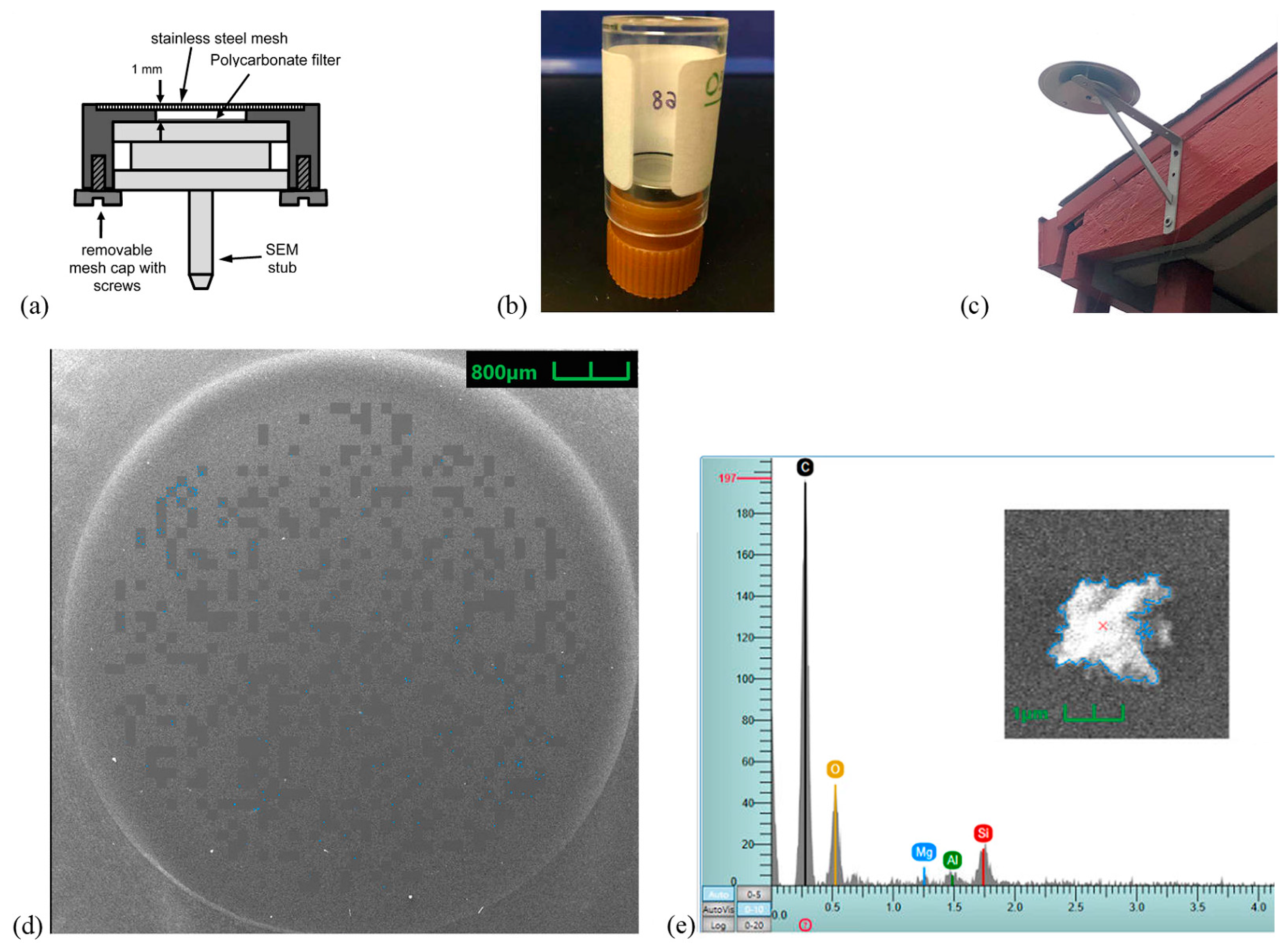
2.1. Sampling Methods

The low-cost, passive PM samplers used in this study (UNC-PAS, RJ Lee Group, Monroeville, PA, USA) (Figure 1a) are about the size of a dime and collect particles onto coated, 0.1 µm pore polycarbonate filter substrates [15]. The sampler collects particles via gravitational settling and diffusion. Mass concentrations are calculated using a particle deposition velocity model that accounts for collection as a function of particle size [8].
UNC-PAS mass size fractions and particle size distributions have shown good co-located precision and correlation with active PM samplers [11,13,16,17].
The passive samplers were transported in single sampler vials (Figure 1b) to and from the site. The indoor samplers were deployed with the vial base as a stand on classroom shelves approximately 2 m high. For outdoor sampling, each passive sampler was deployed inside a weather shelter [18] (Figure 1c).

2.2. Sampling Design

Sampling was conducted at a kindergarten through 8th grade parochial school in Stockton, CA, for two 48 h periods during the first two weeks of December 2021. Due to public health considerations and logistical concerns during the COVID-19 pandemic, all data collection, including the air sampling, was limited to those 48 h periods. The school is in a residential neighborhood surrounded by busy surface roads; an interstate highway 1 mile to the west; and the Port of Stockton, an industrial area with heavy shipping and rail traffic 3 miles away.
Three passive PM samplers were deployed by field staff in two indoor classrooms and one outdoor location on the school premises (Figure 2) as a pilot addition to the larger SAPEP study. The two classrooms A and B were chosen such that they enabled comparison with other SAPEP air measurements, and between rooms with and without air cleaners; Classroom A had a portable air cleaner (IQAir Health Pro Plus) running during the study period while classroom B did not. In both classrooms, doors were typically open and windows were closed. Classroom A was a prefabricated, portable, semi-permanent classroom equipped with an HVAC system that had an ill-fitting MERV 6 filter (gaps were observed) and minimal outside air ventilation. Classroom B was a permanent structure with an HVAC that appeared to have a well-fitting MERV 6 filter and functional outdoor air supply.
Passive PM samplers were co-located with continuous PM2.5 sensors and a pair of BC sensors in all locations. The PM2.5 devices were low-cost nephelometers (Purple Air PA-II, Draper, UT, USA) that utilized a community-developed, continuously updated algorithm that regresses against local PM2.5 beta attenuation monitors and environmental conditions [19]. The BC devices were low-cost aerosol absorption photometers (Aerosol Black Carbon Detectors (ABCD), precommercial version) that have been validated previously in lab and field studies [20]. Due to device registration issues, the PM2.5 sensors only operated during the final 32 h of the 48 h passive sampling period during the first week but covered the entire 48 h sampling period during the second week (hereafter referred to as Week 1 and Week 2).
Two unexposed samplers from the same lot as the field samples were inspected using SEM as laboratory blanks and were analyzed using computer-controlled SEM-EDS (CCSEM-EDS) to blank-correct the sample results.

2.3. CCSEM-EDS Analysis

Particle size and elemental chemistry were measured with a field emission SEM (Tescan MIRA3, Brno) with EDS (Bruker Quantax, Billerica, MA, USA) and automated analysis software (IntelliSEM v1, RJ Lee Group, Monroeville, PA, USA). 500 microscope fields were selected randomly by the IntelliSEM for each sample, and data were collected for each individual particle (Figure 1d,e).
See Appendix A for details on the CCSEM-EDS analysis parameters and airborne PM concentration calculations. Briefly, CCSEM-EDS data from each analyzed sample were input into a custom software algorithm that calculated PM size fractions (PM2.5, PM10–2.5 (PM between 2.5 and 10 μm) and PM10 (PM < 10 μm)), elemental size distributions, mass size distributions, and chemical types [4]. All PM concentrations were blank-corrected by subtracting the average of the two blanks. Blank calculations used the nominal sampling duration (T = 48 h). Particle types were defined using a combination of the automated chemical types and a review of the acquired micro-images’ particle size and morphology.

3. Results

3.1. Airborne Particle Types

The number of particles analyzed via CCSEM-EDS ranged from 200 to 1000 particles per passive sample. Observed particle sizes, morphology, and CCSEM-EDS chemical types are shown in Figure 3, Figure 4, Figure 5, Figure 6, Figure 7, Figure 8 and Figure 9. Together, these data suggest five major airborne particle types: (a) fine, carbonaceous combustion agglomerates, 20 nm–10 μm w/20–200 nm primaries (Figure 3); (b) coarse, biogenic, carbonaceous particles, 1–10 μm (Figure 4); (c) fine iron (Fe)-, chromium (Cr)-, and nickel (Ni)-rich particles, 250 nm–2 μm (Figure 5); (d) predominantly coarse, aluminosilicate soil, dust, and crustal particles, 1–10 μm (Figure 6); and (e) sodium (Na) salt fog particles with associated calcium (Ca), sulfur (S), and/or chlorine (Cl), 200 nm–6 μm (Figure 7).
Figure 8 shows elemental size distributions that are consistent with the above particle types and sizes. Carbonaceous particles (“CO only” in Figure 8 and Figure 9) include both particle types (a) and (b) above. Week 1 carbonaceous size distributions were distributed bimodally, corresponding to fine combustion and coarse biogenic particles. Week 2 carbonaceous and salt particles exhibited more flattened shapes, possibly due to moisture from the 38 mm (1.5 in) of rain recorded at the nearby Holt station during Week 2 sampling; only 0.5 mm (0.02 in) was recorded during Week 1 [21]. The sizes of these flattened carbonaceous and salt particles were likely underestimated due to the low contrast with the substrate in the flat areas (see Figure 7 for an example of a flattened salt particle). The morphology and sizes of the biogenic particles in Figure 4 are generally consistent with fungal spores, hyphae, or other plant fragments [22].
Figure 9 summarizes the compositions of CCSEM-EDS chemical types in each sample. In the PM2.5 fraction, salt particles were the most prevalent chemical type in most samples, with a mean and standard deviation of 44 +/− 18% salt per sample. The next most common PM2.5 types were crustal particles (25 +/− 15%) and carbonaceous (17 +/− 12%). The most prevalent particle types in the PM10–2.5 fraction were crustal (54 +/− 18%), carbonaceous (27 +/− 17%), and salt particles (13 +/− 10%). Of the less common types, unclassified (misc) particles ranged from 9.5 +/− 4.3% to 1.3 +/− 2.5% of the mass in PM2.5 and PM10–2.5, respectively, and metal-rich particles ranged from 4.1 +/− 3.4% to 2.2 +/− 4.9% of the mass in PM2.5 and PM10–2.5, respectively. Phosphorus (P)-, Cl-, and potassium (K)-rich particles were the smallest constituents of these samples, ranging from 0.5 +/− 0.9% to 3.1 +/− 7.0% of the mass in PM2.5 and PM10–2.5, respectively. The P-, Cl-, and K-rich chemical class indicates agricultural fertilizers, plant fragments, and biomass ash and thus represents components of the crustal, biogenic, and combustion particle types described above.
Salt particle compositions and morphologies varied somewhat between the two weeks (Figure 7). In Week 1, the observed salts were mostly Na plus S, with some particles exhibiting Na only and no observed Cl. Fine Na and S curves were measured in all samples (Figure 8). In one sample (Classroom B Week 1), several submicrometer Ca-S particles were also observed, sometimes with a minor Na component, indicating fine gypsum (Figure 8). These hygroscopic particles exhibited a typical morphology of fine spherical or cubic crystals arranged in localized deposits, or “halos”, around a central particle, a pattern caused by their crystallization under vacuum from their original droplet form [13]. In Week 2, salt compositions were more evenly split between sodium plus sulfur, sodium, and sodium chloride. Similar to the carbonaceous particles, Week 2 exhibited more flattened, larger salt recrystallization morphologies (Figure 7).
The two blanks did not possess sulfur-rich salt particles of any of the above types. However, both possessed 1–2 larger (5 μm) S-Cl particles each (see Section 4.2).

3.2. PM Concentrations, Size Distributions, and Comparison to Continuous Sensors

Table 1 presents blank-corrected passive PM concentrations, which ranged from 2.6 to 12.3 μg/m3 for PM2.5 and from 0.5 to 4.6 μg/m3 for PM10–2.5. The average and standard deviations of the blanks for PM2.5 and PM10–2.5 were 1.6 ± 2.0 and 0.3 ± 0.4 μg/m3. The first 48 h period outdoor sampler was damaged during retrieval from the shelter and could not be analyzed.
Measured PM size distributions from Week 1 (Figure 10) show that submicron PM dominated the sample from Classroom B, while the sample from Classroom A had substantial coarse PM. The PM size distributions during Week 2 were similar between both classrooms and the outdoor sample, but Classroom A’s concentration was the lowest. These relationships are also reflected in the calculated PM concentration size fractions in Table 1, which show the lowest PM2.5 in Classroom A during both weeks. The room differences for coarse PM10–2.5, however, were inconsistent.
Two-day averages and trends for the hourly PM2.5 sensor data are presented in Table 1 and Figure 11, respectively. Passive PM2.5, sensor PM2.5, and continuous sensor BC all show similar trends of lower values in Classroom A vs. B, and Week 2 vs. 1. The exception was Classroom A during Week 2, for which PM2.5 sensor data showed the highest average concentration and several prominent peaks. These excursions were not observed in the BC sensor, suggesting either non-BC PM2.5 composition, PM2.5 variation within the classroom, or PM2.5 sensor malfunction.
Overall, passive PM2.5 averaged 4.1 μg/m3 lower than the continuous sensors in pairwise comparisons across all samples (−59%). Note that the Week 1 comparison is limited by incomplete PM2.5 sensor data (32 instead of 48 h). Outdoor PM2.5 measured with a local air district beta attenuation monitor (BAM) approximately 2 mi away (Stockton-University) [23] averaged 17 mg/m3 during Week 1. This is slightly higher than the 12.3 mg/m3 measured using the Week 1 passive sampler in the classroom without an air cleaner (Classroom B); the outdoor passive sampler was damaged in Week 1. The outdoor BAM PM2.5 average of 4.5 mg/m3 during Week 2 was only slightly lower than the passive PM2.5 values for Outdoor C (5.1 mg/m3) and Classroom B (4.9 mg/m3).

4. Discussion

4.1. Combustion and Biogenic Particles

The combustion PM observed in this study had somewhat unusual morphologies, suggesting inefficient combustion, low temperatures, and amorphous organic carbon (Figure 3). These particles are more consistent with smoldering biomass compared with high-temperature combustion (diesel and other engine fuels) [24,25], but they possessed more irregular, agglomerated forms. These particles were observed in both weeks and at all sample locations. The agglomerate in Figure 3a exhibited uniquely large primary particles up to 1 mm in diameter and may represent an unusually heavy organic carbon mass coating or possibly a mixed agglomerate of combustion and biogenic material.
In rare cases, silicon (Si)-dominated 2–3 μm particles with a submicron structure were observed, suggesting ash [26] (Figure 12). The particle in Figure 12b had measurable fluorine (F), suggesting a possible plastic source. Together, these particles suggest impacts from a low-to-medium-temperature burning source. These particles are consistent with smoke from nearby open burning reported during Week 1 approximately 100 m away, though better characterization of that source (and any other nearby combustion sources) and prevailing winds would be needed to link them further.
The lower passive sampler concentrations compared to the PM2.5 sensors (though still within 5 μg/m3) are consistent with previous studies that have observed overestimation from PM2.5 sensors, depending on the algorithm used [27]. In addition, Castillo et al. [13] found that combustion-dominated passive samples analyzed at CCSEM-EDS accelerating voltages of 20 kV yielded lower concentrations than continuous monitors due to reduced detection of combustion PM at this voltage. Despite the detection of fine combustion particles in this study at 20 kV, it is possible that the smallest carbonaceous, submicron particles were under-detected (e.g., smaller diesel PM). When wildfires are expected to be a dominant source, additional 5 kV analyses are recommended to improve detection of this particle type, and have yielded good correlation with organic carbon-rich smoke particles [25]. Nevertheless, the generally good agreement between PM2.5 measured with passive samplers and regional BAM data suggests that any underestimation of mass concentrations was minimal.
The presence of biogenic spore particles in these samples is not unusual for indoor and outdoor environments and is consistent with other studies that have identified particle types in air samples (e.g., [11,13]). Spores and pollen grains may be further identified at the genus level—or in some cases, species or group levels—and may be useful for epidemiology studies targeting allergy and asthma [28].

4.2. Salts

All detected S-rich particles were observed in combination with Na, Na plus Cl, or Ca. Based on the strong morphological evidence of associated water, we hypothesize that these S-rich salt particles are secondary aerosols formed via heterogeneous reactions of Na, Cl, and Ca ions in fog droplets with S from local or regional sources.
One possible source of saline fogs is from San Francisco Bay [29], traveling inland via the Sacramento–San Joaquin River Delta, though local radiation fogs are also common in the Stockton area in the winter months [30]. Average relative humidity was >95% during both weeks [21]. Another potential source is resuspension and rehumidification of sodium hypochlorite aerosols from disinfecting misters that were used historically in this school.
Gypsum (CaSO4) is a common, natural constituent of coarse soil particles, but the extremely fine gypsum particles observed in one sample suggest fog processing of calcium ions together with S, a process analogous to flue gas desulfurization [31].
Two potential S sources of note are several petroleum refineries in neighboring Contra Costa County to the west (gaseous compounds including hydrogen disulfide and sulfur dioxide), as well as local storage facilities for refinery biproducts (solid sulfate powders or elemental S). The latter biproducts are trucked in and out of the Stockton area and stored in uncovered piles on the order of 30,000 tons each, where they are ultimately shipped out of the Port of Stockton as agricultural products [32,33]. These pilings are located approximately 3.5 miles upwind of the school site.
A potential confounder in these results is the rare 5 μm S-Cl particles observed in the blanks, potentially from detergents or personal care products. Although these particles differed substantially from the Na-Cl-S particles in the samples in terms of both their prevalence and size, it is hypothetically possible that any S and Cl contamination could disperse over the substrate and contribute to the S-rich salts in the samples. However, three observations suggest that any such contributions were minimal: (1) EDS acquired from substrate regions with no particles yielded no sulfur; (2) most non-salt particles contained no sulfur; (3) a passive sampler from the same production batch but deployed in a different study in a different location (San Jose, CA, USA) exhibited NaCl particles without S.
The slightly different salt morphologies observed during Week 2 are consistent with the higher droplet water content and the heavier rain reported that week. The rain in Week 2 may also be consistent with the higher proportions of Cl in the Week 2 salt particles if it reduced the residence time of these particles in the air and thus the amount of S that could be incorporated into airborne salt droplets.

4.3. Particles in Classroom A Compared to Classroom B

Passive sampler PM2.5 data (Table 1) show that the room with the portable air cleaner (Classroom A) had lower fine-particle concentrations than Classroom B in both weeks, averaging 5.4 μg/m3 lower (−66%). Coarse PM10–2.5 room differences showed no clear trend; PM10–2.5 was 2.9 μg/m3 higher (130%) in Classroom A than Classroom B in Week 1 but 0.3 μg/m3 lower (−12%) in Week 2. Classroom A exhibited lower passive PM2.5 and PM10–2.5 than the outdoor sample (Week 2), consistent with the BC sensor results, which also showed continuously lower BC in Classroom A than outdoors. Although there is a greater likelihood of combustion BC sources outdoors (with the exception of indoor candles or cooking), their typical particle size range is associated with high penetration efficiency indoors [25]. As such, the lower concentrations in Classroom A still suggest the portable air cleaner was effective. In Classroom B, which was not equipped with an air cleaner, indoor concentrations were only slightly lower than outdoors for both the passive and continuous data.
The CCSEM-EDS data show that Classroom A, Week 1 PM10–2.5 particles were primarily Al-Si soil and dust (Figure 8 and Figure 9). In addition, numerous fine Fe-Cr, Cr, and Fe-Ni particles were present in the Week 1, Classroom A sample (Figure 5a–h). Although dust and metal particles were most prevalent in Classroom A, Week 1, the presence of some dust and minor metals is common and was observed in all environmental samples (Figure 5 and Figure 6). The enhanced presence of coarse PM10–2.5 and metals in Classroom A during Week 1 suggests a potential local PM source such as dust resuspension or heated materials with metal content such as reinforced candle wicks. During week 1, there were evening activities reported in Classroom A, potentially involving lit candles.

4.4. Limitations

The 48 h passive sampling approach necessitated by the overall logistics of this study yielded adequate data quality to determine qualitative particle types and room PM comparisons. However, two days is towards the low end of the 1–90 day range employed in previous studies of similar environments, and thus yielded up to 10 times lower counts [13]. However, the counts in this study were comparable to previous 24 h samples in slightly more polluted areas [11]. The major limitation of short passive sampling durations in lower-PM environments is reduced particle collection, which limits detection of rare particle types and yields poor statistics in the form of high Poisson counting error [11]. The limited passive deployment in this work precluded co-located samplers to verify precision, but the average number of counts, N, implies a Poisson error (=N−1/2) for PM2.5, PM10–2.5, and PM10 of 5.9%, 35%, and 5.8%, respectively. This is comparable to the precision previously reported for passive samplers deployed for less than 1 week [11].
A second impact of short passive durations and reduced sample collection is the greater potential influence of any contamination observed in the blanks. In addition, the blank PM concentrations of 1.6 and 0.3 μg/m3 for PM2.5 and PM10–2.5, respectively, were high compared to the relatively low ambient concentrations at this site. Future study designs with longer sampling times would decrease the blank concentration and detection limit linearly with time, e.g., a 2 week duration would yield detection limits that are seven times lower than 2 days. Future study designs that allow for longer passive sampling times (>1 week) would increase the value of the passive sampling approach. In cases where return sampler retrieval visits are not possible on this timescale, the samples can be retrieved by participants and mailed to the lab [34].
Finally, the predominance of airborne, hygroscopic salt, and gypsum in these samples is associated with variable quantitation uncertainties [9]. Depending on the humidity present during sampling, recrystallization of droplets into dried deposits of much smaller particles can lead to errors in detection, counting statistics, particle volume, and deposition velocity.

5. Conclusions

This work utilized electron microscopy and passive PM samplers to identify particle types based on their particle size, elemental chemistry, and morphology, and also to help interpret continuous pollutant data from low-cost air monitors.
The determination of major airborne particle types in a given environment makes this technique a useful and unique community exposure assessment tool, even in an extremely limited deployment such as this work. The five major particle types identified with CCSEM-EDS, in descending concentrations, were Na salt droplets with S and/or Cl; aluminosilicate dusts; fine, carbonaceous combustion agglomerates and coarse biogenic particles; and fine Fe-, Cr-, and Ni-rich particles. The fine carbonaceous PM observed in this study had unusual morphologies suggesting inefficient combustion, consistent with reported smoke from nearby open burning, though better characterization of that source, any other nearby combustion sources, and prevailing winds would be needed to link them further. We hypothesize that the numerous observed S-rich salt particles are secondary aerosols formed via the reaction of NaCl fog droplets with S from local or regional sources.
The passive PM samplers and continuous PM2.5 and BC sensors show similar trends of lower PM in a classroom equipped with a portable air cleaner, and during the week in which rain was reported. Enhanced PM10–2.5 crustal particles and fine metal particles suggested a potential local PM source in that room, consistent with short-term peaks observed in the PM2.5 sensor data. These findings will help with the interpretation of the broader findings of the SAPEP study when they become available.
Passive PM2.5 concentrations showed generally good agreement with regional reference monitors. As with any lower-cost PM device, however, passive PM2.5 concentrations are best used for comparing relative trends and locations, as opposed to absolute values for health or regulatory purposes. Future studies incorporating more extensive passive sampling in additional classrooms, outdoors, in different seasons, and near regional sources would add more capabilities to future studies.

Author Contributions

Conceptualization, A.B. and J.W.; methodology, A.B., R.C. and J.W.; software, J.W.; validation, J.W.; formal analysis, J.W.; investigation, A.B. and J.W.; resources, J.W.; data curation, R.S., M.T. and J.W.; writing—original draft preparation, J.W.; writing—review and editing, A.B., R.C., S.H., E.M.N., R.S., M.T. and J.W.; visualization, J.W.; supervision, J.W.; project administration, R.C., S.H. and K.K.; funding acquisition, R.C. and S.H. All authors have read and agreed to the published version of the manuscript.

Funding

This research was funded by the Office of Environmental Health Hazard Assessment (OEHHA), Agreement Number 19-E0019.

Institutional Review Board Statement

All study instruments and activities were approved by the State of California Committee for the Protection of Human Subjects with reliance obtained from the UC Berkeley Committee for the Protection of Human Subjects (i.e., the Institutional Review Boards (IRBs)). (CPHS project number: 2021-081; date of approval: 25 August 2021). The study was consistent with the guidelines of the Declaration of Helsinki.

Informed Consent Statement

Informed consent was obtained from all subjects involved in the study.

Data Availability Statement

The data summarized in this study are available on request from the corresponding author. The particle database data are not posted publicly due to their file sizes and operating system requirements but can be exported according to each request.

Acknowledgments

We thank the schoolteachers, staff, and families who participated in SAPEP, without whom this work would not be possible. We thank Thomas Kirchstetter and Chelsea Preble of the Lawrence Berkeley National Laboratory and UC Berkeley for providing the Aerosol Black Carbon Detectors. The findings and conclusions in this article are those of the authors and do not necessarily represent the views or opinions of the California Department of Public Health, the California Health and Human Services Agency, the California Environmental Protection Agency, or OEHHA.

Conflicts of Interest

The authors declare no conflict of interest.

Appendix A. Passive Sampler Analysis Details

Passive sampler SEM-EDS analyses were conducted using secondary electron (SE) and backscattered electron (BSE) detectors. SE imaging is sensitive primarily to sample topography, while BSE imaging is sensitive primarily to atomic number. Before analysis, a carbon coating was applied to all samples for enhanced conductivity and imaging. The SEM was operated in high-vacuum mode at a working distance of 10 mm. Manual SEM-EDS was used to inspect each sample prior to CCSEM-EDS.
CCSEM-EDS was run using a 20 kV accelerating voltage, a beam intensity of 10, a micro-image dwell time of 10 μs, and the SE detector. Manual quality assurance checks of each CCSEM-EDS dataset were performed to check for false negatives or false positives due to filter pores or segmentation of particles larger than 10 µm.
A custom code incorporating a validated, size-dependent deposition model was used to calculate deposition rates and convert the CCSEM-EDS particle count, size, and elemental chemistry data into PM2.5, PM10–2.5, PM10, mass size distributions, and elemental concentration size distributions [8]:
PM i = n = 1 N E i , n P M n = n = 1 N E i , n F n v d e p , n = 1 T n = 1 N E i , n m p , n A s , n v d e p , n
where PMi is either PM2.5 or PM10, Ei,n is the particle-size-dependent, US EPA PM2.5 or PM10 inlet efficiency multiplier for particle n [9], PMn and Fn are the concentration and mass flux contributions from a single particle n, N is the total number of measured particles, T is the sampling duration, mp,n is the mass of particle n [=πρp,n dev,n3/6], dev,n is the equivalent volume diameter of particle n [=dpa,n/Sv], Sv is the assumed volume shape factor (=1.6), ρp is the assumed particle density (=2.0 g/cm3), dpa,n, is the projected-area-equivalent diameter of particle n (=[4 × projected area/π]1/2), and As,n is the substrate area scanned during the analysis for the particle size range including particle n. The particle-size-dependent deposition velocity to the sampler substrate for particle n is defined as follows [35]:
v d e p , n = P c × v t +   D X d × 1 P c + x c / x d   × E c a p
where Pc = porosity of the UNC-PAS cap screen = 0.30, D is the Brownian diffusion coefficient, Xd = distance between cap screen and collection substrate = 0.982 mm, and Xc = cap screen thickness = 0.132 mm. When sampling in low winds indoors or inside the weather shelter, the ambient deposition velocity to the outside of the cap vt is assumed to equal the gravitational settling velocity (=τg), where τ = ρ0 da2Cc/18μ, μ is the dynamic viscosity, g is the gravitational acceleration constant, Cc is the Cunningham correction factor, ρ0 is unit particle density, da (= d e v ρ p C c , d e v ρ 0 C c , d a S d 1 / 2 ) is the aerodynamic particle diameter, and Sd is the dynamic shape factor (=1.4). The minimum detectable particle size for automated acquisitions was da = 0.1 μm.
Individual elemental size distributions were generated by multiplying each particle mass by the measured weight percent of the given element, and were not blank corrected to allow comparison to blank elemental size distributions. All inorganic weight percents were corrected for the non-negligible contribution of the substrate carbon background to the beam X-ray excitation volume using the particle-size-dependent correction factor of Wagner et al. (2012) [11]. Primarily carbonaceous particles (“CO only” in Figure 8) were defined as particles with carbon plus oxygen elemental weight percents = 99% or higher. CO-only size distributions were generated by multiplying each carbonaceous particle mass by 100%.
The custom code automatically assigned each particle one of six chemical types based on its measured elemental weight percents, and then generated corresponding pie charts [7]: (1) Cr, Ni, copper (Cu), or lead (Pb)-containing particles (“metal-rich”); (2) carbonaceous (“CO only”, defined as above), indicative of soot, organic carbon, and plant matter; (3) greater than 2% non-aluminum-silicate K, P, or non-sea-salt Cl (“K, P, Cl”), indicative of agricultural sources and biomass ash; (4) aluminum silicates and Si or calcium oxides, unless they contain P or non-sea-salt Cl (“Crustal”); (5) Na-containing particles (“Salt”); and (6) all others particles (“Misc.”). Chemical-type pie charts were then generated by calculating the relative mass percentages for each size fraction.

References

  1. Murray, C.J.; Aravkin, A.Y.; Zheng, P.; Abbafati, C.; Abbas, K.M.; Abbasi-Kangevari, M.; Abd-Allah, F.; Abdelalim, A.; Abdollahi, M.; Abdollahpour, I.; et al. Global burden of 87 risk factors in 204 countries and territories, 1990–2019: A systematic analysis for the Global Burden of Disease Study 2019. Lancet 2020, 396, 1223–1249. [Google Scholar] [CrossRef] [PubMed]
  2. Gaffney, A.W.; Himmelstein, D.U.; Christiani, D.C.; Woolhandler, S. Socioeconomic Inequality in Respiratory Health in the US From 1959 to 2018. JAMA Intern Med. 2021, 181, 968–976. [Google Scholar] [CrossRef] [PubMed]
  3. Holm, S.; Miller, M.D.; Balmes, J.R. Health Effects of Wildfire Smoke in Children and Public Health Tools: A Narrative Review. J. Expo. Sci. Environ. Epidemiol. 2021, 31, 1–20. [Google Scholar] [CrossRef] [PubMed]
  4. Jandacka, D.; Durcanska, D. Seasonal Variation, Chemical Composition, and PMF-Derived Sources Identification of Traffic-Related PM1, PM2.5, and PM2.5–10 in the Air Quality Management Region of Žilina, Slovakia. Int. J. Environ. Res. Public Health 2021, 18, 10191. [Google Scholar] [CrossRef]
  5. Ayres, J.G.; Borm, P.; Cassee, F.R.; Castranova, V.; Donaldson, K.; Ghio, A.; Harrison, R.M.; Hider, R.; Kelly, F.; Kooter, I.M.; et al. Evaluating the toxicity of airborne particulate matter and nanoparticles by measuring oxidative stress potential—A workshop report and consensus statement. Inhal. Toxicol. 2008, 20, 75–99. [Google Scholar] [CrossRef]
  6. Fussell, J.C.; Franklin, M.; Green, D.C.; Gustafsson, M.; Harrison, R.M.; Hicks, W.; Kelly, F.J.; Kishta, F.; Miller, M.R.; Mudway, I.S.; et al. A Review of Road Traffic-Derived Non-Exhaust Particles: Emissions, Physicochemical Characteristics, Health Risks, and Mitigation Measures. Environ. Sci. Technol. 2022, 56, 6813–6835. [Google Scholar] [CrossRef]
  7. Croft, D.P.; Zhang, W.; Lin, S.; Thurston, S.W.; Hopke, P.K.; van Wijngaarden, E.; Squizzato, S.; Masiol, M.; Utell, M.J.; Rich, D.Q. Associations between source-specific particulate matter and respiratory infections in New York state adults. Environ. Sci. Technol. 2020, 54, 975–984. [Google Scholar] [CrossRef]
  8. Wagner, J.; Leith, D. Passive Aerosol Sampler. Part I: Principle of Operation. Aerosol Sci. Technol. 2001, 34, 186–192. [Google Scholar] [CrossRef]
  9. Ott, D.K.; Cyrs, W.; Peters, T.M. Passive measurement of coarse particulate matter. J. Aerosol Sci. 2008, 39, 156–167. [Google Scholar] [CrossRef]
  10. Wang, Z.M.; Zhou, Y.; Gaspar, F.W.; Bradman, A. Using low cost open-face passive samplers to sample PM concentration and elemental composition in childcare facilities. Environ. Sci. Process. Impacts 2020, 22, 1502–1513. [Google Scholar] [CrossRef]
  11. Wagner, J.; Naik-Patel, K.; Wall, S.; Harnly, M. Measurement of ambient particulate matter concentrations and particle types near agricultural burns using electron microscopy and passive samplers. Atmos. Environ. 2012, 54, 260–271. [Google Scholar] [CrossRef]
  12. Wagner, J.; Casuccio, G. Spectral Imaging and Passive Sampling to Investigate ParticleSources in Urban Desert Regions. Environ. Sci. Process. Impacts 2014, 16, 1745–1753. [Google Scholar] [CrossRef] [PubMed]
  13. Castillo, M.; Kinney, P.; Wagner, J.; Freedman, F.; Eisl, H.; Casuccio, G.; West, R.; Wang, Z.; Yip, K. Field testing a low-cost passive aerosol sampler for long-term measurement of ambient PM2.5 concentrations. Atmos. Environ. 2019, 216, 116905. [Google Scholar] [CrossRef]
  14. OEHHA. California Environmental Protection Agency Office of Health Hazard Assessment. 2021. Available online: https://oehha.ca.gov/calenviroscreen/report/calenviroscreen-40 (accessed on 28 June 2023).
  15. Wagner, J.; Macher, J.M. Comparison of a Passive Aerosol Sampler to Size-Selective Pump Samplers in Indoor Environments. Aiha J. 2003, 64, 630–639. [Google Scholar] [CrossRef]
  16. Maiko, A.; Leith, D. Precision of PM Measurements with the UNC Passive Aerosol Sampler. J. Aerosol Sci. 2013, 57, 161–164. [Google Scholar]
  17. Peters, T.M.; Sawvel, E.J.; Willis, R.; West, R.R.; Casuccio, G.S. Performance of Passive Samplers Analyzed by Computer-Controlled Scanning Electron Microscopy to Measure PM 10–2.5. Environ. Sci. Technol. 2016, 50, 7581–7589. [Google Scholar] [CrossRef] [PubMed]
  18. Ott, D.K.; Peters, T.M. A Shelter to Protect a Passive Sampler for Coarse Particulate Matter, PM 10–2.5. Aerosol Sci. Technol. 2008, 42, 299–309. [Google Scholar] [CrossRef]
  19. SJVAir Collaborative. 2021. Available online: https://www.sjvair.com/about/testing (accessed on 22 September 2023).
  20. Caubel, J.J.; Cados, T.E.; Kirchstetter, T.W. A New Black Carbon Sensor for Dense Air Quality Monitoring Networks. Sensors 2018, 18, 738. [Google Scholar] [CrossRef]
  21. California Irrigation Management Information System (CIMIS) Database, California Department of Water Resources. Available online: https://cimis.water.ca.gov/ (accessed on 21 May 2023).
  22. Wagner, J.; Macher, J. Automated Spore Measurements Using Microscopy, Image Analysis, and Peak Recognition of Near-Monodisperse Aerosols. Aerosol Sci. Technol. 2012, 46, 862–873. [Google Scholar] [CrossRef]
  23. US EPA AirNowTech Database. 2023. Available online: https://www.airnowtech.org/data/ (accessed on 7 November 2023).
  24. Pósfai, M.; Gelencsér, A.; Simonics, R.; Arató, K.; Li, J.; Hobbs, P.V.; Buseck, P.R. Atmospheric tar balls: Particles from biomass and biofuel burning. J. Geophys. Res. 2004, 109, D06213. [Google Scholar] [CrossRef]
  25. Sparks, T.; Wagner, J. Composition of Particulate Matter During a Wildfire Smoke Episode in an Urban Area. Aerosol Sci. Technol. 2021, 55, 734–747. [Google Scholar] [CrossRef]
  26. Adachi, K.; Dibb, J.E.; Scheuer, E.; Katich, J.M.; Schwarz, J.P.; Perring, A.E.; Mediavilla, B.; Guo, H.; Campuzano-Jost, P.; Jimenez, J.L.; et al. Fine ash-bearing particles as a major aerosol component in biomass burning smoke. J. Geophys. Res. Atmos. 2022, 127, e2021JD035657. [Google Scholar] [CrossRef]
  27. Wallace, L.; Zhao, T.; Klepeis, N.E. Calibration of PurpleAir PA-I and PA-II Monitors Using Daily Mean PM2.5 Concentrations Measured in California, Washington, and Oregon from 2017 to 2021. Sensors 2022, 22, 4741. [Google Scholar] [CrossRef]
  28. Hjelmroos-Koski, M.K.; Macher, J.M.; Katharine Hammond, S.; Tager, I. Considerations in the grouping of plant and fungal taxa for an epidemiologic study. Grana 2006, 45, 261–287. [Google Scholar] [CrossRef]
  29. Gundel, L.A.; Benner, W.H.; Hansen, A.D. Chemical composition of fog water and interstitial aerosol in Berkeley, California. Atmos. Environ. 1994, 28, 2715–2725. [Google Scholar] [CrossRef]
  30. Herckes, P.; Marcotte, A.R.; Wang, Y.; Collett, J.L., Jr. Fog composition in the Central Valley of California over three decades. Atmos. Res. 2015, 151, 20–30. [Google Scholar] [CrossRef]
  31. Ma, Q.; He, H.; Liu, Y.; Liu, C.; Grassian, V.H. Heterogeneous and multiphase formation pathways of gypsum in the atmosphere. Phys. Chem. Chem. Phys. 2013, 15, 19196–19204. [Google Scholar] [CrossRef]
  32. Stockton Record, Piles of Sulfur at Port of Stockton. 28 May 1996. Available online: https://www.recordnet.com/story/news/1996/05/28/piles-sulfur-at-port-stockton/50854338007/ (accessed on 21 November 2022).
  33. California Regional Water Quality Control Board, Central Valley, Revised Monitoring and Reporting Program No. R5-2008-0825. 2008. Available online: https://www.waterboards.ca.gov/centralvalley/board_decisions/adopted_orders/san_joaquin/r5-2008-0825_mrp_rev.pdf (accessed on 15 November 2023).
  34. Harnly, M.; Naik-Patel, K.; Wall, S.; Quintana, P.; Pon, D.; Wagner, J. Agricultural burning: Air monitoring and exposure reduction in Imperial County. Calif. Agric. 2012, 66, 85–90. [Google Scholar] [CrossRef]
  35. Nash, D.G.; Leith, D. Ultrafine Particle Sampling with the UNC Passive Aerosol Sampler. Aerosol Sci. Technol. 2010, 44, 1059–1064. [Google Scholar] [CrossRef]
Figure 1. (a) Schematic of passive PM sampler. (b) Shipping vial. (c) Outdoor weather shelter. (d) CCSEM-EDS overview image showing random field selection (small dark squares) and detected particles (blue dots). (e) Example of individual particle record including EDS data.
Atmosphere 14 01702 g001
Figure 2. Sampling map of the school site showing A and B indoor classroom locations and outdoor sampling location C.
Atmosphere 14 01702 g002
Figure 3. Carbonaceous combustion agglomerates, 20 nm–10 μm w/20–200 nm primary particles. (a,b) Room A, week 1. (c,d) Room B, week 1. (e,f) Room A, week 2. (g,h) Room B, week 2. (i,j) Outdoor C, week 2. See Section 4.1 for discussion of the primary sizes in (a).
Atmosphere 14 01702 g003
Figure 4. Biogenic particles, 1–10 μm. (a,b) Room A, week 1. (c,d) Room A, week 2. (e,f) Room B, week 2. (g) Outdoor C, week 2.
Atmosphere 14 01702 g004
Figure 5. Fine metal particles. (ah) Classroom A, week 1. (i,j) Flat particles in Classroom B, week 1. (k) Fragment in Classroom A, week 2. (l) Fragment in blank sample.
Atmosphere 14 01702 g005
Figure 6. Typical coarse aluminosilicate PM10–2.5 particles in Classroom A, week 1, and EDS spectrum from left particle showing aluminum (Al), Si, and minor Na, K, Ca, and Fe.
Atmosphere 14 01702 g006
Figure 7. Low magnification SEM images showing clusters of submicron, Na (S, Cl, and Ca) salt particles in samples from Classroom A, week 1, and Classroom B, week 2, but absent from blank. Magnified examples of individual particles from each sample are shown in the second row, along with an extremely rare, 5 μm S-Cl particle from a blank sample average.
Atmosphere 14 01702 g007
Figure 8. Elemental size distributions (size bin-normalized mass concentrations (μg/m3) vs. aerodynamic diameter (μm)) calculated for all sampling locations and blank average. Primarily carbonaceous particles are also included and denoted “CO only”. The arrows on the X axes denote 2.5 μm.
Atmosphere 14 01702 g008
Figure 9. Percentage of chemical types per sample by mass for (a) PM2.5 and (b) PM10–2.5. The size of each pie chart is scaled by the non-blank-corrected mass concentration. See Appendix A for particle type definitions.
Atmosphere 14 01702 g009
Figure 10. PM size distributions (size bin-normalized mass concentrations (μg/m3) vs. aerodynamic diameter (μm)) for outdoor Week 2 and both classrooms during Weeks 1 and 2.
Atmosphere 14 01702 g010
Figure 11. Continuous PM2.5 and BC sensor data for the three locations and two sampling periods. Each BC time series represents the average of two co-located BC sensors.
Atmosphere 14 01702 g011
Figure 12. (a,b) Two Si-dominated 2–3 μm particles with submicron-fine structure, suggesting ash. Both are from the Classroom B, week 2 sample.
Atmosphere 14 01702 g012
Table 1. Sampling information, PM2.5 sensor averages, and passive sample PM results.
Week NumberSample DatesDescriptionPM2.5 Sensor Avg (μg/m3)Sample IDPassive Samples (Blank-Corrected)
PM2.5 (μg/m3)PM10–2.5 (μg/m3)PM10 (μg/m3)
15 December 2021–7 December 2021Classroom A7.869403.93.47.3
Classroom B13.6694712.30.512.8
Outdoor C17.96948n/a an/a an/a a
212 December 2021–14 December 2021Classroom A12.369442.62.04.6
Classroom B7.669494.92.37.2
Outdoor C7.969435.14.69.7
a Sample malfunction, not analyzed.
Disclaimer/Publisher’s Note: The statements, opinions and data contained in all publications are solely those of the individual author(s) and contributor(s) and not of MDPI and/or the editor(s). MDPI and/or the editor(s) disclaim responsibility for any injury to people or property resulting from any ideas, methods, instructions or products referred to in the content.

