Article

Vertical Profile of Meteoric and Surface-Water Isotopes in Nepal Himalayas to Everest’s Summit

1
State Key Laboratory of Tibetan Plateau Earth System, Resources and Environment (TPESRE), Institute of Tibetan Plateau Research, Chinese Academy of Sciences, Beijing 100101, China
2
Central Department of Hydrology and Meteorology (CDHM), Tribhuvan University, Kathmandu 44600, Nepal
*
Author to whom correspondence should be addressed.
Atmosphere 2023, 14(2), 202; https://doi.org/10.3390/atmos14020202
Submission received: 29 November 2022 / Revised: 30 December 2022 / Accepted: 17 January 2023 / Published: 18 January 2023
(This article belongs to the Section Meteorology)

Abstract

:
This study presents isotopic compositions and their vertical profile of meteoric and surface water samples collected in the Southern Himalaya since 2015, with elevations extending all the way up to Mt. Everest’s summit. The data covering a wide altitudinal ranges and rich water types are presented for the first time. The series of in situ samples up to 8848 m asl lead to the following discoveries: (1) the dominance of rainy-season precipitation to surface-water composition in the Southern Himalaya, (2) the high correlation and high similarity between meteoric and surface-snow isotopes, thus implying the representation of surface-snow isotopes to high-elevation climatology, (3) a significant altitude effect in river and ground water, with the higher altitudinal lapse rate in ground water δ18O highlighting strong local impacts on the vertical profile of surface-water isotopes, (4) different transitions suggested by the vertical profiles of δ18O variation in snow and ice in the Southern Himalaya, with the transition in snow δ18O at a vertical zone between 6030 and 6280 m asl, and that in ice at 5775 m asl, and (5) complex circulation processes on top of the Himalaya, featuring the interaction of large-scale circulation with local mountain valley circulation, katabatic wind, and sublimation in the extremely cold and high environment. They, thus, confirm the correlation between isotopes and altitudes in regions influenced by complex circulation patterns to clarify the altitude effect, and suggest the application of isotopic study/isotopic chemistry in geological study.

1. Introduction

The Tibetan Plateau and its surroundings host the largest ice mass outside the conventional polar regions (i.e., the Arctic and Antarctica) [1]; thus, it is known as the Asian water towers [2]. As alpine glaciers mainly grow in extremely high elevations, the appreciation of glacial mass balance requires a comprehensive understanding of air temperature and precipitation variation features with altitude in the mountainous terrain. Ground-based meteorological observations rely on automatic weather stations (AWSs) and field expeditions with penetrating radar and boreholes in the Southern Himalaya, and help shed light on unique variation features of various meteorological variables with altitude, suggesting elevation-dependent variation in major meteorological variables, including precipitation, temperature, humidity, and radiation between 2600 and 5600 m above sea level (later abbreviated as asl) (e.g., [3,4]). The elevation-dependent warming (EDW) was first proposed to indicate that the increase in warming rate with altitude would have a devastating effect on alpine glaciers [4]. The integration of station data with remote sensing data also supports this understanding, as Qin et al. [5] detected the halting of temperature decrease at altitudes up to around 5000 m asl, beyond which the temperature was found to increase with altitude. Yet, recent integration by Zhang et al. [6] suggested that that EDW is only valid up to about 5000 m, followed by reversed altitudinal patterns above 5000 m to 6500 m, and attributed the reversed altitudinal pattern below and above 5000 m to the persistent snow cover that prohibits an increase in warming rate with increasing height. The resolution of such a controversy relies on the better understanding of local meteorological conditions; yet, establishing and maintaining meteorological observation stations under such harsh environments are challenging and sometimes even dangerous.
Due to the temperature dependence of water isotopes during phase transformation, the altitudinal lapse rate of temperature is translated to the altitude effect of water-stable isotopes in meteoric and surface waters. Earlier datasets in IAEA-GNIP facilitated the detection of the altitude effect in precipitation isotopes, discovering the depletion of the heavy oxygen isotopes with elevation as ranging between 0.1 and 0.5‰ per 100 m and primarily resulting from the cooling of the air masses as they ascend a mountain, accompanied by the rainout of the excess moisture [7]. Such an isotopic feature has been widely used in the reconstruction of paleoelevations [8], and successful examples can be found with the understanding of the uplift history of the Tibetan Plateau [8,9,10] and Cordillera [11]. A recent controversy also arose, quoting atmospheric circulation as capable of influencing the altitudinal lapse rate [12]. Indeed, the altitude effect of water isotopes is mainly attributed to the Rayleigh effect as dominating the water-phase transformation, while other factors besides the basic Rayleigh effect may also change the isotope composition [7]. Surface-water sampling in and around the region also suggests the weakening [13], or even reverse [14], of the altitude effect in water isotopes under complicated atmospheric-circulation dominance. Those controversies highlight the importance of clarifying the altitude effect in complex topography and extremely high elevations, as it concerns the validity and robustness of applying the isotope altitude effect to paleoelevation reconstruction in the earth’s history.
The importance of large-scale atmospheric circulation on the altitude effect has been proposed in previous studies, although no consensus has been reached regarding the exact altitude for the emergence of the transition in the elevation-dependent variations [15]. Some studies (e.g., [16]) found the monsoon climate, particularly the wind circulation variation which is closely linked to the monsoon onset [17], is significantly affecting the meteorological conditions in the Southern Himalaya between 2600 and 5600 m asl. While other studies found the different wind circulations at different elevations, characterized by the down-slope winds at low elevations, leading to enhanced precipitation as the enhancement of surface convergence prevents drying [15], whereas significant diurnal variations at high elevations [17] resulting in reduced precipitation at high elevations due to the enhancement of nocturnal down-slope winds under warming [15]. Isotopes in water, as they participate in water-phase transformation during the water cycle, are a direct recorder of atmospheric circulations. Regarding the surface accumulation of glaciers in the atmospheric complex region on the Tibetan Plateau, it has a topographic-dependent feature that is subject to post-deposition processes including wind scouring, condensation, ablation, sublimation, etc. [18]. Yet, the lack of field observations and coexistence of complex geographical factors (such as cloud and glaciers) obstruct the validation of remote sensing data and reanalysis data, which have too-coarse grid spacing and are unnecessary for resolving orographic flow patterns [15].
Water-stable isotopes stand out as a natural bond in linking local hydrological status to large-scale and local atmospheric circulations, as the vapor pressure differs at the surface versus in the atmosphere. The difference may vary under various circulation and transportation conditions, thus directly affecting the isotopic composition in precipitation and surface water. Various studies [19,20,21,22] have confirmed water-stable isotopes as an efficient tracer of moisture trajectory and atmospheric status.
Compared to meteorological monitoring in extremely high altitudes (>5500 m asl) that requires continuous duty, surface water along the mountain slopes is relatively easy to sample. The Sagarmāthā National Park lies in the Himalayas of Eastern Nepal which is dominated by Mount Everest, extending to Dudh Kosi River in the south and the peak of Qomolangma in the north. It experiences the most dramatic elevation rise (from 1000 to 8848 m asl) within a short distance of about 30 km, and hence holds the key to understanding elevation-dependent variations in both atmospheric circulation and local processes, which ultimately contributes to better appreciating the past and future of the Himalayan environment.
This study presents a series of first-hand sampling data along Khumbu Valley in the Nepal Himalayas, hoping to present a comprehensive understanding of the altitude effect on meteoric and surface water in the Southern Himalayan region. A better understanding of the spatial and temporal variation features of water-stable isotopes in the topographically complex regions is expected to contribute to (1) verifying the close link between isotopes and local meteorological conditions and attempting to use surface-water sampling and isotopic study in the study of elevation-dependent warming. Additionally, (2) confirming the correlation between isotopes and altitudes in regions influenced by complex circulation patterns to clarify the altitude effect, and make suggestions on the application of isotopic study/isotopic chemistry in geological study.

2. Materials and Methods

Making use of the popular trekking route in the Khumbu Valley, Nepal Himalaya, this study collaborated with Nepalese Sherpa mountaineers to focus on both fixed-sited precipitation and extensive field surface-water sampling along the route, and aimed to present a comprehensive understanding of the altitude effect in water-stable isotopes, taking interannual, seasonal, and topographic factors into consideration. Since 2014, several field campaigns have been conducted along the Khumbu Valley in the Nepal Himalayas, setting up fixed-sited precipitation-sampling sites and acquiring river, ground water, snow, and ice samples from the southern plain to the peak of Qomolangma. The high-elevation precipitation-sampling site was located at Lobuche (86.8 ºE, 27.9 ºN, 5050 m asl; Figure 1), in collaboration with Nepal Academy of Sciences. The local staff was asked to collect event-based precipitation, with liquid precipitation directly poured into 15 mL PET bottles before tightly screwing, and snow samples melted at room temperature before undergoing the same practice as the liquid samples. The precipitation onset date and start and finish time were also recorded according to local time.
Meanwhile, we carried out the surface-water sampling at moderate elevations, and also asked local Sherpa mountaineers to sample mainly in the Khumbu Glacier, which originates in the western Cwm near Everest, flows westwards in a great fall of seracs before turning southwards to form a tongue that descends to an altitude of 3900 m (Figure 1). In those field campaigns, water was collected from rivers, trickles, ponds, snow surface, and ice using a 15 mL (for liquid) or 30 mL (for solid) polyethylene bottle. The geographical locations of the sampling sites were determined using a hand-held Garmin 639 s. The upper limit of the surface-water sample has been pushed up to Mt Everest’s summit (8848 m asl).
All samples from fields are well-preserved in the cold natural environment at Lobuche before being transported to Beijing, China for measurement in the Lab of Tibetan Environmental Changes and Land surface processes. The lab measurement was performed on Picarro Li2101 using the cavity ring-down system, with the precision for δ18O as ±0.1‰ and ±0.5‰ for δ2H.
The deuterium excess (d) is a secondary parameter in isotope hydrology and is calculated as:
d = δ2H − 8 × δ18O
The local meteoric water line (LMWL) of precipitation or local evaporation line (LEL) of surface water is calculated by linearly regressing δ18O against δ2H for respective elevation ranges and/or seasons.
Sampling sites are binned to elevation ranges every 50 m and presented by the median value of each bin, so as to clearly show the altitudinal variation profile of surface-water isotopes.
To find the change point in δ18O variation with altitude, we used the ruptures package in Python, and applied four methods, i.e., the Pelt search method, the binary segmentation search method, the window-based method, and dynamic programming search methods. Through comparing those outputs, we eye-picked those with clear and concise changes. The transitions were then double-checked using other isotopic features including the δ2H-δ18O regression and d18O correlations.
To better understand local climate controls and possible large-scale atmospheric circulation impacts on water-stable isotopes, we resorted to station historical data at the Pyramid International Laboratory/Observatory high-altitude scientific research center, as well as updated reanalysis data including NCEP/NCAR reanalysis, ERA5, CRU TS4., and GHND2. SRTM was also downloaded to give an impression of the sampling-domain topography.

3. Results

3.1. Precipitation Stable Isotopes

Daily precipitation stable isotopes during 2016–2018 showed wide variation amplitude in both δ18O (ranging over 30‰) and d (ranging over 60‰) values. The climatology demonstrated a distinct intra-annual variation, highlighting low δ18O (median = −20‰) and d (<10‰) values during February, generally high δ18O (median > −10‰) concomitant with a decreasing d median value from 25‰ in May to 17‰ in June, and low δ18O and d values during July–September (Figure 2).
The LMWL for daily precipitation during July–September showed much lower slopes (<8) and intercepts (<5), but much higher slopes (>8.2) and intercepts (>10) during May–June. These variations are the result of a number of factors, the foremost being the origin and rainout history of the precipitating air mass, the rain intensity and cloud structure, as well as the degree of evaporation during the descent of the rain droplets to the ground beneath the cloud base, are also important factors.
Such a distinct intra-annual variation in precipitation stable isotopes corresponds well with metrological climatology based on hourly data during 2004–2008, as July–September featured much higher precipitation and temperature than in other months, implying a rainy season associated with the summer monsoon circulation (Figure 2b). Meanwhile, as precipitation increased dramatically from May to June, contemporary δ18O increased while d decreased, probably attributable to the increasing relative humidity, as the adjoining ocean provides the major moisture source during the monsoon season. February witnessed the lowest δ18O in precipitation, which corresponded to the lowest air temperature of the year, suggesting the temperature effect is dominant during dry seasons (Figure 2c).
To better link the surface water with the meteoric water, this study mainly focuses on climate controls during rainy seasons and ignores climatic controls over precipitation during dry seasons (November–April), given the latter’s minimal contribution to annual accumulation. There was a significant negative correlation between δ18O and temperature during June (slope: −5.1‰/°C, p < 0.01), whereas it was positive during July (slope: 1.93‰/°C, p < 0.05) and September (slope: 7.81‰/°C, p < 0.01). The negative temperature–δ18O correlation coexists with the amount effect widely present in tropical regions during intense convection [23], while the positive correlation during the full-blown phase of the summer monsoon is worth noticing. Previous studies in monsoon domains have also focused on such a phenomenon, and concluded that zero thermal uplift during the mature monsoon evolution might play a role in the temperature effect on precipitation δ18O [24].

3.2. Surface Waters

Both river and ground water showed little difference in altitude effect regardless of month. The vertical-variation gradient of δ18O in river water varied from −0.14‰/100 m in May to −0.16‰/100 m in November (Table 1 and Figure 3). The altitude effect of ground water was larger than that in river water, which might be associated with the local effect that subjects ground water to the local climate status. The altitude-δ18Ogradient varied from −0.24‰/100 m (−0.25‰/100 m) during November (May) to −0.37‰/100 m during January. Given the much lower temperature in January than other months, the significantly higher temperature from May to October probably contributes to the melting of permafrost. Consequently, the mixing of ice and snow melt with ground water in higher altitudes might lead to the further depletion of ground water isotopes in higher altitudes.
The variation in ice and snow isotopes with altitude was comparatively more complex: there was increasing ice but decreasing snow δ18O with altitude throughout the year (Table 1). As water in high, cold regions has a low change ratio and long stay period, the combination of old and fresh snow δ18O yielded a significant altitudinal lapse rate in snow in the Nepal Himalaya as −0.33‰/100 m (R = −0.48), which was much larger than that in regional river or ground water, but similar to that in surface water in the extensive Asian monsoon domain (16–30 ºN, 77–98 ºE) during the non-monsoon (−0.32‰/100 m) [25]. There was no significant altitude effect on ice δ18O (Table 1).
The overlay of surface-snow samples on contemporary precipitation at Lobuche (5050 m asl) shows large similarity in their isotopic compositions (Figure 4). Statistical analyses using cross-correlation from the statsmodels package (https://www.statsmodels.org/stable/generated/statsmodels.tsa.stattools.ccf.html, accessed on 26 December 2022) show the two time series are significantly correlated within a two-day lag. Particularly, the surface-snow δ18O in 2016 was strongly positively correlated with precipitation δ18O within a two-day lag (R value, the correlation co-efficiency, is 0.96 at lag 0, decreasing to 0.76 at lag 1, and further to 0.56 at lag 2), and similarly with the correlation in 2017 (R = 0.81 at lag 0, decreasing to 0.72 at lag 1 and 0.48 at lag 2). Note, however, that the cross-correlations were not significant in 2018. The much lower δ18O value in May of 2018 was probably associated with the fact that the surface-snow-sample location was 300 m lower in elevation than the precipitation-sampling sites and, hence, the possible altitudinal lapse effect. Despite the identical meteoric δ18O (medians for 2016 and 2017 are, respectively, −16.4‰ and −13.1‰) and d (medians for 2016 and 2017 are, respectively, 10.7‰ and 11.7‰) values at Lobuche station from 2016 to 2017, δ18O in the corresponding ice collected between 5000 and 5600 m showed wide amplitude (~18 ‰) and distinct interannual variations (higher in 2016 than that in 2017 by nearly 20‰ in median values). This suggests a distant link between ice and corresponding precipitation, as the old ice probably records the precipitation in past years.
The vertical variation in snow and ice isotopes along slopes will be the foci of the following discussions, as they are abnormal and complex, extend up to extremely high elevations, and have rarely been reported for such an altitudinal level.

4. Discussion

4.1. Possible Transition Suggested by Vertical Profile of Surface Snow and Ice Isotopes

To avoid possible biases due to seasonality impacts on surface-snow isotopic variation, we only report samples collected in May for the vertical profile of δ18O (Figure 5). From Figure 5, it is found that the altitudinal range does not directly determine the snow δ18O variation amplitude, as the year 2017 of the widest sampling elevation range failed to witness the most δ18O variation, but instead showed an annual δ18O value close to that in 2016 (Figure 4a). Additionally, note that the altitudinal level for surface-snow sampling was not the highest in 2018, yet the corresponding δ18O values were generally lower than in other years, which is largely associated with three outliers that can be considered as normal in the previous two years (Figure 5a). All those interannual-variation features in surface-snow δ18O suggest the superimposition and mixture of snow between succinct years. Hence, the interannual variation in surface-snow δ18O may mean less for interannual variation in atmospheric circulations, but more of a general status of dominant circulations/trajectories over the altitudinal range. We will attempt to discuss this issue in Section 4.3. Unlike snow δ18O, ice δ18O showed no clear interannual or seasonal variations (Figure 5b), which was due to the different physical features and formation mechanisms between the two [26].
The vertical profiles of surface water δ18O in 50 m elevation bins highlight large standard deviations in surface-snow δ18O (Figure 5c), which is probably related to the large interannual variation in surface-snow samples, and suggests possible transitions in the altitudinal lapse rates of ice δ18O around 6000 m asl (Figure 5d). This highlights the necessity to distinguish between snow and ice in the discussion of their vertical profile along the Southern Himalayan slope.

4.2. Detection of the Transitional Altitudes and Attributions

As aforementioned, we focused on snow samples in May only and calculated the sample δ18O anomalies by removing the means before dividing them by the standard deviation (Figure 6). The application of checkpoint detection in machine learning helps identify the altitudes where possible transitions occur. The transitional zone for surface-snow δ18O values was found between 6030 and 6280 m asl (Figure 6a). Surface snow below 6030 m asl showed a significant (p < 0.01) altitudinal lapse rate for δ18O at −0.78‰/100 m (R = −0.48) (Figure 6(c1)), corresponding to a high δ2H-δ18O linear regression slope (8.46) and intercept (18.83) (Figure 6(c2)). The variation gradient of δ18O with altitude was much larger than previously reported for the Tibetan Plateau and its surroundings during non-monsoon (−0.32‰/100 m, [25]), and for the Yungas–Altiplano transect during the rainy season (~0.25‰/100 m; [27]). Other larger variation gradients (e.g., −1.0‰/100 m) were only found from the combination of summer rainfall δ18O across stations (ranging from 2400 to 4200 m asl) on the Pacific slope of the Andean Cordillera in Northern Chile [27,28] with those reported by Fritz et al. [29]. The patently larger δ18O–altitude gradient, hence, may be attributed to complex moisture sources.
Those above 6280 m asl showed a significant (p < 0.05) increase in δ18O with altitude at 0.30‰/100 m (R = 0.66) (Figure 6(c1)). Previous studies (e.g., [26]) have shown that in extremely cold cases, deposition (i.e.vapor transforms directly to ice) might take place, leading to heat release, and this probably explains the positive slope of surface-snow δ18O with altitude beyond the transitional zone. Correspondingly, the δ2H-δ18O regression showed a much lower slope and intercept, probably associated with the partial rainout from the vapor reservoir with increasing altitude [30] (Figure 6(c2)). The reversed d18O correlations below and beyond the transition zone are also worth noting, as the coexistence of depleted δ18O values with high d (correlation coefficient, R, as −0.82 at the 99% confidence level) in surface-snow samples above 6280 m (Figure 6(c3)) suggests the Jouzel–Merlivat effect during snow formation in a colder environment [20]. The positive d18O correlation in the lower elevation zone (R = 0.54, p < 0.01), otherwise, corresponds to the high δ2H -δ18O slope and intercept and probably reflects precipitation condensation at high relative humidity associated with the abundant marine vapor supply [31]. The distinct δ18O variation features, meteoric-water lines, and d18O correlations with altitudinal groups confirm the stark contrast in surface-snow isotopic compositions, and imply possible transitions in the atmospheric circulation or local land surface processes in those elevation zones. The field account in the 1950s showed that the altitudinal range between 6000 and 7500 m witnessed a powdery snow field where the refreeze of snow was common [32]. Surface snow in the transition zone features a δ2H -δ18O slope of 8.01 and intercept of 13.9, generally close to the GMWL [21] (Figure 6(c2)), while the wide amplitude of δ18O and lack of significant correlation between d and δ18O (Figure 6(c1,c3)) suggest the effect of wind drifting. Specifically, the monsoon precipitation in the form of snow at higher elevations would be whipped up and cascaded off the steep slope in this elevation zone, resulting in a possible mixture of snow from different moisture sources with wind scouring and fresh snow relocation [32]. Thus, caution should be used when interpreting the vertical-variation features of surface-snow δ18O in the transition zone.
Checkpoint detection clearly identified 5775 m asl as a transition in the vertical lapse rate of ice δ18O, with its covariation gradient increasing by 3.6‰ per 100 m increase in elevation (R = 0.68, p < 0.01) below, with a gradient of −0.32‰/100 m (R = −0.55, p < 0.01) above the transition (Figure 6(d1)). Despite the overall declining trend in ice δ18O with altitude beyond 5775 m asl, there are noticeable fluctuations, such as the persistent increase from −16.83‰ in 6680 m to −3.65‰ in 7330 m asl, implying complex interactions between large-scale atmospheric and local mountain circulations. The remarkable discrepancy in precipitation seasonality between the Dasuopu glacier (7200 m) and the East Rongbuk glacier (6518 m asl) in the Central Himalayas [33] demonstrates the complex atmospheric circulations in this elevation zone.
The comparison of the δ2H-δ18O linear regression lines between lower and higher elevation zones is opposite in ice to that in surface snow, featuring a much higher slope and intercept beyond (slope = 8.32) than below (slope = 7.46) the transition (Figure 6(d2)). The high δ2H -δ18O slope in ice above 5775 m asl is identical to the slope in surface snow below 6030 m asl, both close to the slope yielded by condensation by isobaric cooling for an initial temperature of 0 °C [34]. This is usually associated with closed-system conditions under equilibrium fractionations [35]. Compared with the high relative humidity for surface snow in lower elevations, winds were mainly out of the northeast near Everest’s summit [36], with the cold continental wind further cooling the region. Both conditions would lead to high δ2H-δ18O slopes, as there is a negative correlation between temperature and δ2H-δ18O slope, with more than eight slopes corresponding to a low condensation temperature [37] and/or a lack of secondary evaporation in an extremely cold environment [34].
The transition elevation initiates lower for ice than surface snow in the Southern Himalaya, which underlines the comparative stability of ice versus snow after deposition. Specifically, the transition for ice δ18O falls within the zone of ice pinnacles (5200–5900 m asl) developing on the southeast sides of convexities in the glacier [32], suggesting marine moisture intrusion from the adjoining ocean. The generally steep slope in the Nepal Himalaya may result in more meteoric precipitation in the lower altitudes, which is characterized by very low δ18O and high d due to monsoon convection of marine moisture (Figure 6(d3)) [38,39]. Additionally, it should be noted that the high δ18O near the transition is accompanied by low d (Figure 6(d3)), which is attributable to the latent heat release during melting and refreezing. As snow is usually regarded as material that has not changed much since it fell [26], it might be more closely related to circulation and trajectories, as will be discussed below.

4.3. Circulation Mechanisms Revealed by the Vertical Profile of Surface-Snow Isotopes

The isotopic compositions in surface snow are inherited from those in meteoric water, and, thus, can help reveal atmospheric circulation patterns and contribute to understanding atmospheric transmission over extremely high elevations. The transition zone on the southern slope of the Eastern Himalaya demarcates the vertical profile of surface-snow δ18O-altitude from negative below to positive beyond the transition zone (Figure 6(c1)). Several causes might contribute to the transition: (1) The dominance of monsoon circulation below 6030 m asl, which is suggested by the significant altitude effect, high LEL slope, and intercepts related to equilibrium fractionation during monsoon convection and moisture supply, and significant d-relative humidity anomaly correlation in the eastern equatorial Indian Ocean (Figure 7a). (2) The prevalence of katabatic wind above 6280 m asl, where cooling on the snow-covered plateau would generate a large pressure gradient force that would cause a dramatic temperature decrease on the mountain slope, leading to a dramatic decrease in surface-snow δ18O (Figure 7b). (3) Sublimation in extremely high elevations, where the extremely cold environment induces vapor to deposit on ice, leading to heat release and a temperature increase in the surface snow, hence the increase in snow δ18O with altitude; this can be confirmed by the much lower LEL slope (6.85) and intercept (−7.69) (Figure 6(c2)), usually associated with sub-cloud evaporation under a super-cooled and dry environment (Figure 7c). Additionally, (4) the superimposition of large-scale atmospheric circulation with local valley wind brings about surface-snow disturbances and results in the mixture of precipitation of various sources, hence the wide variation range in surface-snow δ18O in the transitional zone (Figure 6(c1,c3) and Figure 7b).

5. Conclusions

The topographic-dependent feature of glaciers requires a comprehensive understanding of the vertical structure of local and large-scale atmospheric circulations, as they pertain directly to surface accumulation subject to post-deposition processes including wind scouring, condensation, ablation, sublimation, etc. [18]. The lack of field observations and coexistence of complex geographical factors (such as cloud and glaciers), however, obstruct the validation of remote sensing data and reanalysis data, which have too-coarse grid spacing and are unnecessary for resolving orographic flow patterns [15]. Otherwise, the most important water towers are also among the most vulnerable [40]. Such an urgent situation warrants an advanced understanding of glacial mass variations and their driving mechanisms based on solid ground evidence. This study presents isotopic compositions and their vertical profile of meteoric and surface-water samples collected from the Khumbu Valley in the Southern Himalaya since 2015. The rich sample types, repeatable samplings, and wide elevation ranges of those samples ensure a more robust understanding of unique circulation features on the highest mountain peak in the world. The following discoveries are proposed:
(1)
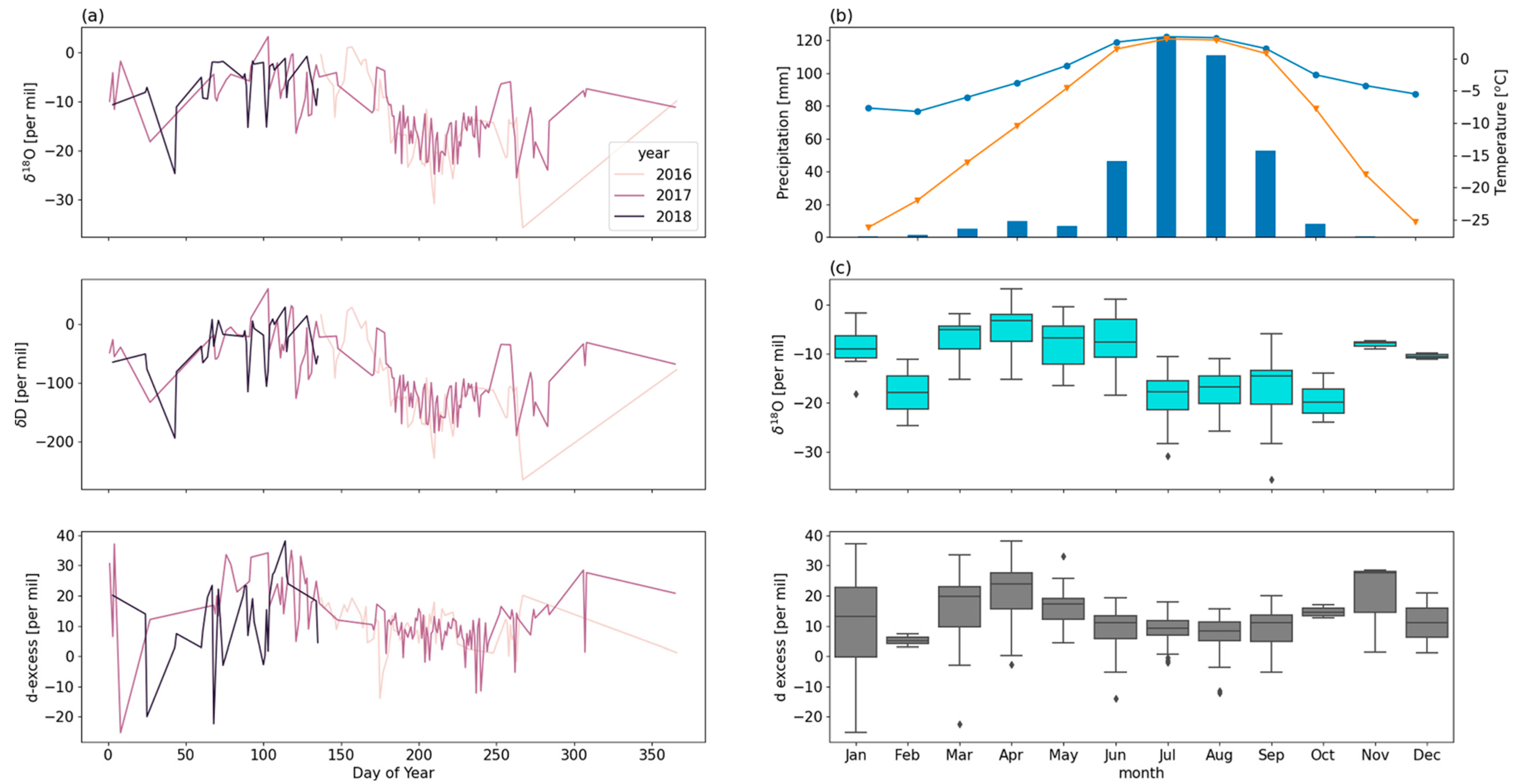
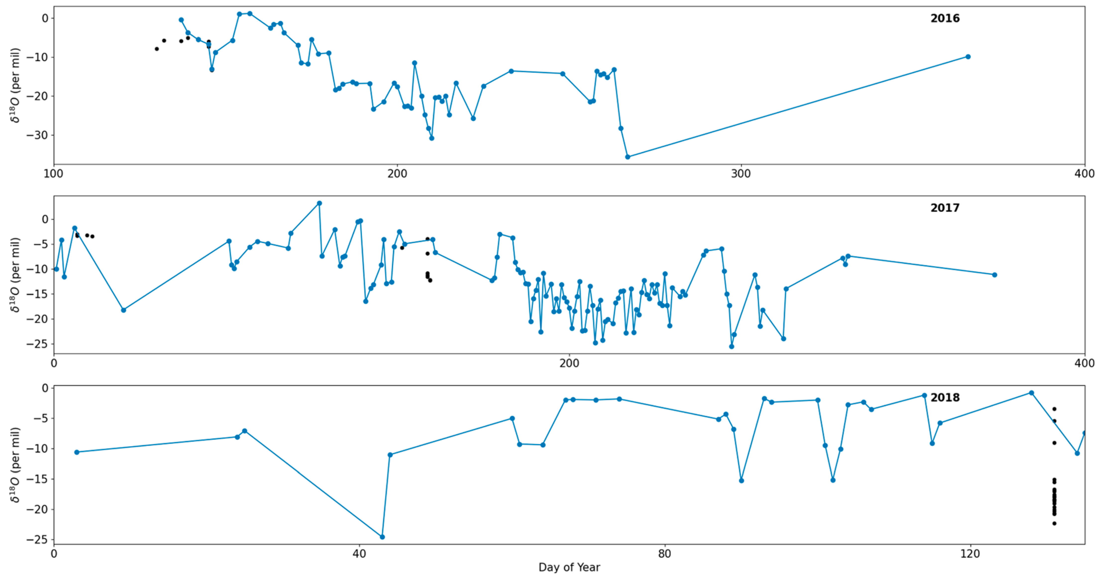
Daily precipitation stable isotopes during 2016–2018 at 5050 m asl confirm the dominance of Indian summer monsoon circulation, highlighting the significance of rainy-season (May–October) precipitation to surface-water composition given the poor precipitation amount during dry seasons (November–April).
(2)
The comparison of surface-snow isotopes with corresponding precipitation data prove the high correlation and high similarity between the two. It also underlines the slow rotation cycle of surface snow and implies the climatic, rather than synoptic, significance of high-elevation surface snow.
(3)
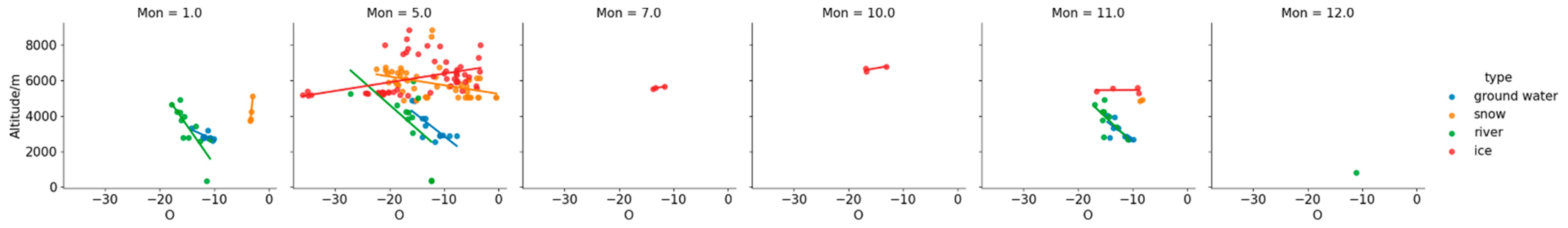
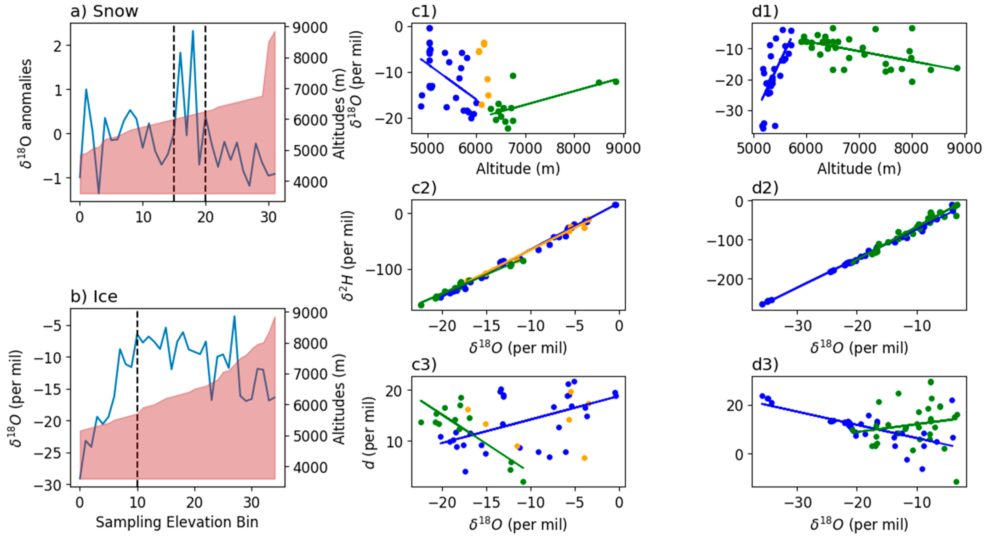
δ18O in both river and ground water sampled below 5500 m asl show a significant altitude effect in the Southern Himalaya, with the altitudinal lapse rate of ground water larger than that of river. This implies strong local impacts on the vertical profile of surface-water isotopes.
(4)
Snow and ice samples were all collected above 5500 m asl; hence, they provide a first glimpse of the altitudinal lapse rate of surface water in extremely high elevations. The vertical profiles of both water types suggest a transition in the altitudinal lapse rate of δ18O, with the transition in snow δ18O at a vertical zone between 6030 and 6280 m asl, while that in ice at 5775 m asl.
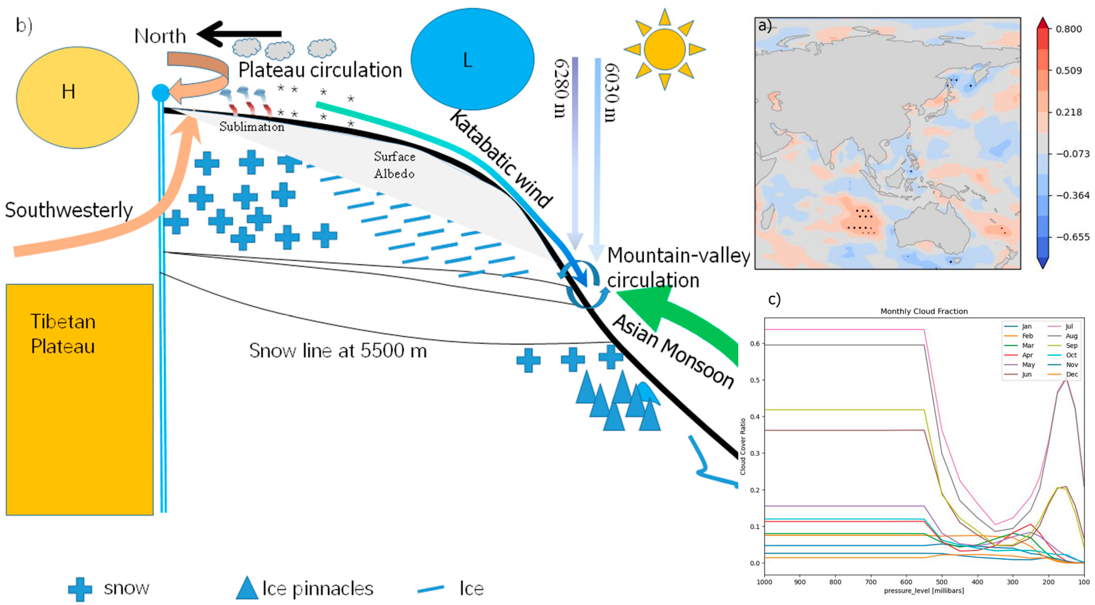
(5)
The vertical profile in surface-snow δ18O also suggests moisture sources and the interaction of large-scale circulation with local mountain valley circulation, katabatic wind, and sublimation in the extremely cold and dry environment on top. We, thus, reveal more complex circulation patterns overpassing the peak of the Himalaya than previously understood. Such a study is also conducive to understanding the deposition effect of a cold and dry environment on atmospheric pollutants, supplementing the current understanding on major wind circulation streams over extremely high elevations, and highlighting the effect of katabatic wind on South Asian transport.
More matching studies in the northern slope of the Himalaya should be conducted to verify the surmounting processes of various atmospheric components (such as black carbon, aerosols, water vapor, precipitation, etc.) over the Qomolangma and, thus, to better comprehend the interaction between atmospheric circulation and complex topography.

Author Contributions

Conceptualization, X.Y.; methodology, X.Y.; formal analysis, X.Y. and S.A.; investigation, X.Y.; resources, X.Y. and S.A.; data curation, X.Y.; writing—original draft preparation, X.Y.; writing—review and editing, X.Y.; visualization, X.Y.; supervision, T.Y.; project administration, T.Y.; funding acquisition, T.Y. All authors have read and agreed to the published version of the manuscript.

Funding

This study was supported by the second Tibetan plateau scientific expedition and research program (grant No. 2019QZKK0208, 2019QZKK0201) and Strategic Priority Research Program of Chinese Academy of Sciences (grant No. XDA20100300).

Informed Consent Statement

Not applicable for studies not involving humans.

Data Availability Statement

The data presented in this study are available on request from the corresponding author.

Acknowledgments

The authors acknowledge Kaji Bista for coordinating sampling along the southern slope of Everest, Dongmei Qu for facilitating the lab analysis, and numerous mountaineers for risking their lives in sampling along their way to the Everest’s summit.

Conflicts of Interest

The authors declare no conflict of interest.

References

  1. Farinotti, D.; Huss, M.; Fürst, J.J.; Landmann, J.; Machguth, H.; Maussion, F.; Pandit, A. A consensus estimate for the ice thickness distribution of all glaciers on Earth. Nat. Geosci. 2019, 12, 168–173. [Google Scholar] [CrossRef] [Green Version]
  2. Immerzeel, W.W.; Van Beek, L.P.H.; Bierkens, M.F.P. Climate change will affect the Asian Water Towers. Science 2010, 328, 1382–1385. [Google Scholar] [CrossRef] [PubMed]
  3. Barros, A.P.; Lang, T.J. Monitoring the Monsoon in the Himalayas: Observations in Central Nepal, June 2001. Mon. Weather Rev. 2003, 131, 1408–1427. [Google Scholar] [CrossRef]
  4. Pepin, N.; Bradley, R.S.; Diaz, H.F.; Baraer, M.; Caceres, E.B.; Forsythe, N.; Fowler, H.; Greenwood, G.; Hashmi, M.Z.; Liu, X.D.; et al. Elevation-dependent warming in mountain regions of the world. Nat. Clim. Chang. 2015, 5, 424–430. [Google Scholar] [CrossRef] [Green Version]
  5. Qin, J.; Yang, K.; Liang, S.; Guo, X. The altitudinal dependence of recent rapid warming over the Tibetan Plateau. Clim. Chang. 2009, 97, 321–327. [Google Scholar] [CrossRef]
  6. Zhang, H.; Immerzeel, W.W.; Zhang, F.; de Kok, R.J.; Chen, D.; Yan, W. Snow cover persistence reverses the altitudinal pat-terns of warming above and below 5000 m on the Tibetan Plateau. Sci. Total Environ. 2022, 803, 149889. [Google Scholar] [CrossRef] [PubMed]
  7. Ingraham, N.L. Chapter 3—Isotopic Variations in Precipitation. In Isotope Tracers in Catchment Hydrology; Kendall, C., McDonnell, J.J., Eds.; Elsevier: Amsterdam, The Netherlands, 1998; pp. 87–118. [Google Scholar]
  8. Ding, L.; Spicer, R.A.; Yang, J.; Xu, Q.; Cai, F.; Li, S.; Lai, Q.; Wang, H.; Spicer, T.E.V.; Yue, Y.; et al. Quantifying the rise of the Himalaya orogen and implications for the South Asian monsoon. Geology 2017, 45, 215–218. [Google Scholar] [CrossRef] [Green Version]
  9. Rowley, D.B.; Garzione, C.N. Stable Isotope-Based Paleoaltimetry. Annu. Rev. Earth Planet. Sci. 2007, 35, 463–508. [Google Scholar] [CrossRef]
  10. Xiong, Z.; Liu, X.; Ding, L.; Farnsworth, A.; Spicer, R.A.; Xu, Q.; Valdes, P.; He, S.; Zeng, D.; Wang, C.; et al. The rise and demise of the Paleogene Central Tibetan Valley. Sci. Adv. 2022, 8, eabj0944. [Google Scholar] [CrossRef]
  11. Feng, R.; Poulsen, C.J.; Werner, M.; Chamberlain, C.P.; Mix, H.; Mulch, A. Early Cenozoic Evolution of topography, climate and stable isotopes in precipitation in the North American Cordillera. Am. J. Sci. 2013, 313, 613–648. [Google Scholar] [CrossRef]
  12. Botsyun, S.; Sepulchre, P.; Donnadieu, Y.; Risi, C.; Licht, A.; Rugenstein, J.K.C. Revised paleoaltimetry data show low Tibetan Plateau elevation during the Eocene. Science 2019, 363, eaaq1436. [Google Scholar] [CrossRef] [PubMed]
  13. Kang, S.; Qin, D.; Yao, T.; Duan, K. High-elevation Meteoric precipitation δ~(18)O features in Xixabangma during summer monsoon (in Chinese with English abstract). J. Mt. Sci. 2000, 1, 1–6. [Google Scholar]
  14. Kong, Y.; Pang, Z. A positive altitude gradient of isotopes in the precipitation over the Tianshan Mountains: Effects of moisture recycling and sub-cloud evaporation. J. Hydrol. 2016, 542, 222–230. [Google Scholar] [CrossRef]
  15. Norris, J.; Carvalho, L.M.V.; Jones, C.; Cannon, F. Warming and drying over the central Himalaya caused by an amplification of local mountain circulation. Npj Clim. Atmos. Sci. 2020, 3, 1. [Google Scholar] [CrossRef] [Green Version]
  16. Yang, K.; Guyennon, N.; Ouyang, L.; Tian, L.; Tartari, G.; Salerno, F. Impact of summer monsoon on the elevation-dependence of meteorological variables in the south of central Himalaya. Int. J. Climatol. 2018, 38, 1748–1759. [Google Scholar] [CrossRef]
  17. Ueno, K.; Toyotsu, K.; Bertolani, L.; Tartari, G. Stepwise Onset of Monsoon Weather Observed in the Nepal Himalaya. Mon. Weather. Rev. 2008, 136, 2507–2522. [Google Scholar] [CrossRef]
  18. de Kok, R.J.; Tuinenburg, O.A.; Bonekamp, P.N.J.; Immerzeel, W.W. Irrigation as a Potential Driver for Anomalous Glacier Behavior in High Mountain Asia. Geophys. Res. Lett. 2018, 45, 2047–2054. [Google Scholar] [CrossRef] [Green Version]
  19. Gat, J.R. Some classical concepts of isotope hydrology: ”Rayleigh fractionation, Meteoric Water Lines, the Dansgaard effects (altitude, latitude, distance from coast and amount effects) and the dexcess parameter”. In Isotopes in the Water Cycle: Present and Future of a Developing Science; Aggarwal, P.K., Gat, J.R., Froehlich, K.F.O., Eds.; Springer: Dordrecht, The Netherlands, 2005; pp. 127–137. [Google Scholar]
  20. Jouzel, J.; Merlivat, L. Deuterium and oxygen 18 in precipitation: Modeling of the isotopic effects during snow formation. J. Geophys. Res. Atmos. 1984, 89, 1749–1757. [Google Scholar] [CrossRef]
  21. Rozanski, K.; Araguasaraguas, L.; Gonfiantini, R. Relation between Long-Term Trends of Oxygen-18 Isotope Composition of Precipitation and Climate. Science 1992, 258, 981–985. [Google Scholar] [CrossRef]
  22. Tian, L.; Yao, T.; Numaguti, A.; Sun, W. Stable Isotope Variations in Monsoon Precipitation on the Tibetan Plateau. J. Meteorol. Soc. Jpn. 2001, 79, 959–966. [Google Scholar] [CrossRef] [Green Version]
  23. Aggarwal, P.K.; Romatschke, U.; Araguas-Araguas, L.; Belachew, D.; Longstaffe, F.J.; Berg, P.; Schumacher, C.; Funk, A. Proportions of convective and stratiform precipitation revealed in water isotope ratios. Nat. Geosci. 2016, 9, 624–629. [Google Scholar] [CrossRef]
  24. Yang, X.; Yao, T.; Yang, W.; Yu, W.; Qu, D. Co-existence of temperature and amount effects on precipitation δ18O in the Asian monsoon region. Geophys. Res. Lett. 2011, 38, 6. [Google Scholar] [CrossRef]
  25. Yang, X.; Xu, B.; Yang, W.; Qu, D. The Indian monsoonal influence on altitude effect of δ 18O in surface water on southeast Tibetan Plateau. Sci. China Earth Sci. 2012, 55, 438–445. [Google Scholar] [CrossRef]
  26. Cuffey, K.M.; Paterson, W.S.B. The Physics of Glaciers; Elservier: Oxford, UK, 2010. [Google Scholar]
  27. Gonfiantini, R.; Roche, M.-A.; Olivry, J.-C.; Fontes, J.-C.; Zuppi, G.M. The altitude effect on the isotopic composition of tropical rains. Chem. Geol. 2001, 181, 147–167. [Google Scholar] [CrossRef]
  28. Aravena, R.; Suzuki, O.; Peña, H.; Pollastri, A.; Fuenzalida, H.; Grilli, A. Isotopic composition and origin of the precipitation in Northern Chile. Appl. Geochem. 1999, 14, 411–422. [Google Scholar] [CrossRef]
  29. Fritz, P.; Suzuki, O.; Silva, C.; Salati, E. Isotope hydrology of groundwaters in the Pampa del Tamarugal, Chile. J. Hydrol. 1981, 53, 161–184. [Google Scholar] [CrossRef]
  30. Gonfiantini, R. On the isotopic composition of precipitation. In Proceedings, International Symposium on Isotope Hydrology, In memory of J.-Ch. Fontes; BRGM-Orstom: Paris, France, 1996. [Google Scholar]
  31. Clark, I.D.; Fritz, P. Environmental Isotopes in Hydrogeology; CRC Press: New York, NY, USA, 1997. [Google Scholar]
  32. Roch, A. The Glaciers, Snow and Avalanches of Mount Everest. J. Glaciol. 1954, 2, 428–430. [Google Scholar] [CrossRef] [Green Version]
  33. Pang, H.; Hou, S.; Kaspari, S.; Mayewski, P.A. Influence of regional precipitation patterns on stable isotopes in ice cores from the central Himalayas. Cryosphere 2014, 8, 289–301. [Google Scholar] [CrossRef] [Green Version]
  34. Dansgaard, W. Stable isotopes in precipitation. Tellus 1964, 16, 436–468. [Google Scholar] [CrossRef]
  35. Kendall, C.; Caldwell, E.A. Fundamentals of Isotope Geochemistry. In Isotope Tracers in Catchment Hydrology; Kendall, C., McDonnell, J.J., Eds.; Elsevier: Amsterdam, The Netherlands, 1998; pp. 51–86. [Google Scholar]
  36. Matthews, T.; Perry, L.B.; Koch, I.; Aryal, D.; Khadka, A.; Shrestha, D.; Abernathy, K.; Elmore, A.C.; Seimon, A.; Tait, A.; et al. Going to Extremes: Installing the World’s Highest Weather Stations on Mount Everest. Bull. Am. Meteorol. Soc. 2020, 101, E1870–E1890. [Google Scholar] [CrossRef]
  37. Majoube, M. Fractionnement en 180 entre la glace et la vapeur d’eau. J. Chim. Phys. 1971, 68, 625–636. [Google Scholar] [CrossRef]
  38. Vuille, M.; Werner, M. Stable isotopes in precipitation recording South American summer monsoon and ENSO variability: Observations and model results. Clim. Dyn. 2005, 25, 401–413. [Google Scholar] [CrossRef] [Green Version]
  39. Wang, D.; Tian, L.; Cai, Z.; Shao, L.; Guo, X.; Tian, R.; Li, Y.; Chen, Y.; Yuan, C. Indian monsoon precipitation isotopes linked with high level cloud cover at local and regional scales. Earth Planet. Sci. Lett. 2020, 529, 115837. [Google Scholar] [CrossRef]
  40. Immerzeel, W.W.; Lutz, A.F.; Andrade, M.; Bahl, A.; Biemans, H.; Bolch, T.; Hyde, S.; Brumby, S.; Davies, B.J.; Elmore, A.C.; et al. Importance and vulnerability of the world’s water towers. Nature 2020, 577, 364–369. [Google Scholar] [CrossRef]
Figure 1. Map of meteoric- and surface-water-sampling sites in the Southern Himalaya. The red square in the upper panel indicate water-sampling area. The red markers in the lower panel demarcate surface-water-sampling sites against the hillslope background downloaded from Shuttle Radar Topography Mission (SRTM).
Atmosphere 14 00202 g001
Figure 2. Variation in δ18O in daily meteoric water at Lobuche and climatic seasonality based on hourly data during 2004–2008. (a) daily time series of meteoric water δ18O at Lobuche during 2016–2018, (b) five-year climatology of precipitation amount (bars), air temperature (blue curve), and dew-point temperature (orange curve) at the station, and (c) monthly boxplot of daily meteoric isotopes during the observation period.
Atmosphere 14 00202 g002
Figure 3. Variation in surface water δ18O with altitude in different months. Numbers on top of each panel represent sampling month.
Atmosphere 14 00202 g003
Figure 4. Overlay of precipitation δ18O (blue dotted curve) with that in surface snow (black dots) collected within a 50 m distance.
Atmosphere 14 00202 g004
Figure 5. Variation in surface-snow sampling in May during the entire sampling program. (a) boxplot of interannual δ18O variation (colored) superimposed on sampling elevation ranges (vertical gray bars) for surface-snow samples, (b) same as (a) but for ice samples, (c) vertical profile of surface-snow δ18O with error bars in elevation bins, (d) same as (c) but of ice δ18O.
Atmosphere 14 00202 g005
Figure 6. Possible transition in the snow/ice δ18O variations with altitude in the Southern Himalaya identified using change point detection. (a) transitional zone detected for surface-snow samples, and (b) same as (a), but for ice samples. (c1c3) vertical lapse rate of δ18O in surface-snow samples with altitude, local evaporation lines (LELs) and correlation of δ18O with d excesses in different elevation ranges; least square linear regression lines are shown, together with corresponding results for significant correlations at 95% confidence level. (d1d3) same as (c1c3), but for ice samples. The brown shadings in (a,b) indicate samples’ elevations. ‘Trans-‘ and ‘Trans + ’ indicate areas, respectively, below and above the transition. Blue, orange, and green dots in (c)s and (d)s indicate samples, respectively, below, within, and above the transitional zone.
Atmosphere 14 00202 g006
Figure 7. Hypothetical mechanisms for the transition and verification using reanalysis data. (a) correlation of anomalies between d excess in snow with relative humidity based on daily data throughout the sample periods, (b) schematic figure of possible circulation streams and interactions on the southern slope of the Himalaya, and (c) cloud fraction over corresponding grid (27.9 ºN, 86.8 ºE) from EAR5.
Atmosphere 14 00202 g007
Table 1. Variation in water-stable isotopes with altitude. Bold numbers indicate correlation covariants significant at 99% confidence level, and italic numbers significant at 95% confidence level. ‘--’ indicates correlation insignificant due to too few samples.
Water TypeAltitude–δ18O Covariant (‰/100 m)Altitude–Deuterium Excess Covariant (‰/100 m)
JanMayJulOctNovDecAllAll
Ground Water−0.37−0.25 −0.24
River−0.14-- −0.16--
Snow--−0.27 -- −0.33−0.19
Ice 0.34------ 0.34--
Disclaimer/Publisher’s Note: The statements, opinions and data contained in all publications are solely those of the individual author(s) and contributor(s) and not of MDPI and/or the editor(s). MDPI and/or the editor(s) disclaim responsibility for any injury to people or property resulting from any ideas, methods, instructions or products referred to in the content.

