Analysis of PM_2.5 Characteristics in Yancheng from 2017 to 2021 Based on Kolmogorov–Zurbenko Filter and PSCF Model

Abstract

Based on the hourly monitoring data including meteorological elements and PM_2.5 mass concentration in Yancheng from 2017 to 2021, PM_2.5 mass concentration variations, influencing factors and source apportionment were studied by the Kolmogorov–Zurbenko filter and Potential Source Contribution Function Analysis (PSCF) method. The results showed that the mass concentration of PM_2.5 in Yancheng showed a decreasing trend from 2017 to 2021, with a decline rate of about 33.8% (2017, 44.79 ± 31.22 μg/m³; 2021, 29.66 ± 21.69 μg/m³); the visibility increased by 18.4% (2017, 11.69 ± 6.46 km; 2021,13.8 ± 6.24 km), which is mainly related to emission reduction measures in China. The mass concentration of PM_2.5 has significant seasonal variation characteristics, with the highest in winter, reaching 60.61 μg/m³, and the lowest in summer, only 23.11 μg/m³. The diurnal variation of PM_2.5 showed a unimodal distribution, and concentration difference is obvious under the influence of land–sea breeze (36.60 μg/m³, easterly wind; 43.57 μg/m³, westerly wind). Meteorological factors have an important impact on the mass concentration of PM_2.5, which fluctuates with seasons. It is calculated to have a good fitting relationship between the visibility and PM_2.5 concentration, and the correlation decreases with the increase in humidity (−0.71 ~ −0.41). The relatively clean atmosphere under high humidity conditions is also prone to the obstruction to vision. The corresponding PM_2.5 concentration varies significantly under different wind directions and wind speeds in Yancheng, and high values mainly come from the northwest–southeast–southwest direction. The potential source regions in autumn are mainly distributed in southwestern Jiangsu and northwestern Zhejiang; the potential source regions in winter are mainly located in southwestern Jiangsu, southern Anhui and northern Jiangxi.

1. Introduction

Atmospheric aerosol refers to all kinds of solid and liquid particulate matter in the atmosphere, in which the aerodynamic equivalent diameter is less than or equal to 2.5 μm, called fine particulate matter, namely, PM_2.5. In recent decades, with the rapid urbanization and industrialization process, a large number of pollutants have been discharged and environmental air quality has deteriorated. PM_2.5 has become an important pollutant affecting urban air quality [1,2]. PM_2.5 stays in the air for a long time and can effectively absorb and scatter solar radiation, which significantly reduces atmospheric visibility [3,4]. Because of its small particle size and large specific surface area, it is easy to carry harmful substances such as polycyclic aromatic hydrocarbons [5,6].

In order to control PM_2.5 pollution, the Chinese government has implemented effective emission reduction measures since 2013. The PM_2.5 mass concentration has decreased significantly, but there are still high-pollution incidents [7,8,9]. Since air quality improved by anthropogenic emission reduction may be affected by meteorological conditions [10], it is of great significance to analyze the influence of meteorological conditions on the change in PM_2.5 concentration. In recent years, a large number of studies have been conducted on the spatial and temporal distribution, influencing factors and source apportionment of PM_2.5 mass concentration. Zhang et al. [11] statistically analyzed the low visibility events in eastern China in January 2013 and found that more than 2/3 of the diurnal changes in fog-haze and heavy pollution weather were caused by meteorological factors. Under stable weather conditions, low near-surface wind speed and high relative humidity are conducive to the accumulation of pollutants [12,13,14]. In addition, regional transport is an important factor in exacerbating local air pollution. Wang et al. [15] used the backward trajectory analysis method to study the source of black carbon aerosol in Beijing, and found that the air mass pollution from Siberia was light and the air mass pollution from North China was more serious. Wang et al. [16] analyzed the large-scale haze process in central and eastern China caused by a cold front transport in the winter of 2019, and found that in the whole process, the local pollutants in Jiangsu accounted for 25.8%, and the pollutants outside Jiangsu accounted for 74.2%, and the contribution of transportation was the main one. Through a three-year observation, Wang et al. [17] found that ambient air quality in Shanghai was mainly affected by air masses in the west, east and north directions, with a high concentration of pollution mainly coming from air masses in the west of the Yangtze River Delta, while air masses from the East China Sea were relatively clean and had the lowest particulate pollution.

Yancheng is located in the central and eastern part of Jiangsu Province, with rich land resources and the main landforms constituted by plains. It is the intersection of the two strategies of national coastal development and the integration of the Yangtze River Delta. Its social and economic development ranks in the middle of Jiangsu Province, and it is also in the stage of steady progress. At present, there are few studies on Yancheng in Jiangsu Province. As a coastal city, Yancheng is frequently affected by local circulation such as sea–land breeze. However, there are few studies on the role of regional transport caused by land and sea differences in the formation of PM_2.5 pollution events in Yancheng. Based on the observation data of PM_2.5 in Yancheng from 2017 to 2021, combined with meteorological data, this paper analyzed its long-term trend and influencing factors, and explored the reasons why obstruction to vision still occurs frequently in Yancheng despite the gradual improvement of air quality. By calculating the mass concentration of PM_2.5 under different wind direction and wind speed, and clustering the backward trajectory, the main direction of pollutants under the influence of local circulation such as sea–land breeze was preliminarily determined. In addition, the concentration weight trajectory analysis was used to study the transmission path and potential source regions of PM_2.5 in Yancheng, in order to provide support for regional air pollution prevention and control.

2. Data and Methods

2.1. Observation Site and Data

The PM_2.5 observation data in this paper were collected from the National Air Quality Environmental Monitoring Platform from 1 January 2017 to 31 December 2021, and the observation station is located in the Municipal Environmental Monitoring Center Station (33.39° N, 120.16° E), No. 7 Wengang North Road, Tinghu District, Yancheng, and the station is mainly surrounded by residential communities, commercial areas and schools. Figure 1a,b, respectively, show the location of Yancheng in Jiangsu and even in China and the environment around the observation station. The observation site is surrounded by Jianjun Road, Huanghai Road, Kaifang Avenue, Qingnian Road Viaduct, Huanghai Road Viaduct and other main roads, and there is a large traffic flow nearby. The meteorological data used in this paper are the same period data from the observation site of Yancheng Meteorological Bureau.

Before the research, the quality control of PM_2.5 data was carried out: 1. Remove the missing and incorrect values (PM_2.5 concentration ≤ 0) of PM_2.5 concentration in the original data; 2. The 3σ rule method was used to remove the outliers; 3. If the number of samples is less than 80% of the total number when calculating the daily average and monthly average PM_2.5 concentration, it would be considered invalid.

In this paper, the seasons are divided according to climatic methods, with spring from March to May, summer from June to August, autumn from September to November, and winter from December, January and February.

2.2. Kolmogorov–Zurbenko Filter

For the daily average concentration X (t) of PM_2.5 in Yancheng it can be decomposed into:

$$X(t)=e(t)+S(t)+W(t)$$

(1)

where e(t) is the long-term variation of PM_2.5 in Yancheng City, S(t) is the seasonal variation, and W(t) is the short-term variation [18,19].

KZ(m, p) filtering was used to extract the daily average PM_2.5 concentration to extract the long-term trend from PM_2.5 data. KZ filtering is a low-pass filtering through p iterations and m point moving average. The calculation formula is as follows:

$$Y_i=\frac{1}{m}{\displaystyle \sum _{-k}^k{X}_{i+j}}$$

(2)

where X is the daily average concentration of PM_2.5 from 2017 to 2021. When X is filtered, the length of sliding windows at both ends is k, m is the length of sliding windows, m = 2k + 1. The result of this filtering will be calculated again as the input variable of the next filtering. This cycle was iterated p times to extract the long-term trend of PM_2.5 in Yancheng.

The filtering parameters m and p can control filtering of processes with different scales. KZ (m, p) filtering removes wave frequencies with wavelength less than N:

$$m\times p^{1/2}\le N$$

(3)

KZ(365,3) filter removes short-term fluctuations with periods less than 632 days (1.7 years), thus obtaining the long-term trend of PM_2.5 in Yancheng.

2.3. Potential Source Contribution Function (PSCF)

The PSCF is a method for identifying the source of pollutants based on airflow trajectory analysis, and is widely used to identify potential source regions [20]. PSCF function is defined as the conditional probability that the corresponding PM_2.5 concentration exceeds the set threshold when the air mass passing through a certain region reaches the observation point. In this paper, the threshold of PM_2.5 concentration is set as 75 μg/m³ (the second grade of national standard). When the corresponding concentration of the trajectory is higher than the threshold, it will be identified as a pollution trajectory. In this paper, the region corresponding to the high PSCF value is the potential source area of PM_2.5 concentration in Yancheng.

Yancheng monitoring station (33.39° N, 120.16° E) was selected as the starting point of the backward track, and the simulated initial height was 500 m. The Hybrid Single-Particle Lagrangian Integrated Trajectory model (HYSPLIT) [21,22] is used to calculate the backward trajectory of air masses arriving at Yancheng monitoring station hourly every day. The mode backward time is 72 h. In this paper, the study area is divided into 0.5° × 0.5° i × j grids. PSCF is used to evaluate the contribution of different regions to PM_2.5 concentration in Yancheng, and the conditional probability of particle concentration exceeding the threshold at the observation point corresponding to the trajectory through the grid is calculated. The calculation method is shown in Formula (4):

$$\mathrm{P}\mathrm{S}\mathrm{C}{\mathrm{F}}_{ij}=\frac{m_{ij}}{n_{ij}}W\left(n_{ij}\right)$$

(4)

$$W(n_{ij})=\{\begin{array}{l}\begin{array}{cc}1.0\begin{array}{cc}\begin{array}{cc}& \end{array}& \end{array}& 3n_{ave}<n_{ij}\end{array}\\ \begin{array}{cc}0.7& 1.5n_{ave}<n_{ij}\le 3n_{ij}\end{array}\\ \begin{array}{cc}0.4& n_{ave}<n_{ij}\le 1.5n_{ave}\end{array}\\ \begin{array}{cc}0.17\begin{array}{cc}& \begin{array}{cc}& \end{array}\end{array}& n_{ij}\le n_{ave}\end{array}\end{array}$$

(5)

where n_ij is the total number of all trajectory endpoints passing through the grid point(i, j), and n_ij is the total number of endpoints whose corresponding pollutant concentration exceeds the set threshold in the trajectory passing through the grid point(i, j). PSCF is a conditional probability function. When n_ij is small, there is greater uncertainty, so the weight function W (n_ij) [23] is introduced.

The data required for PSCF were accessed from the NCEP Global Data Assimilation System database (GDAS1).

3. Results and Discussion

3.1. Time Variation of PM_2.5 Mass Concentration

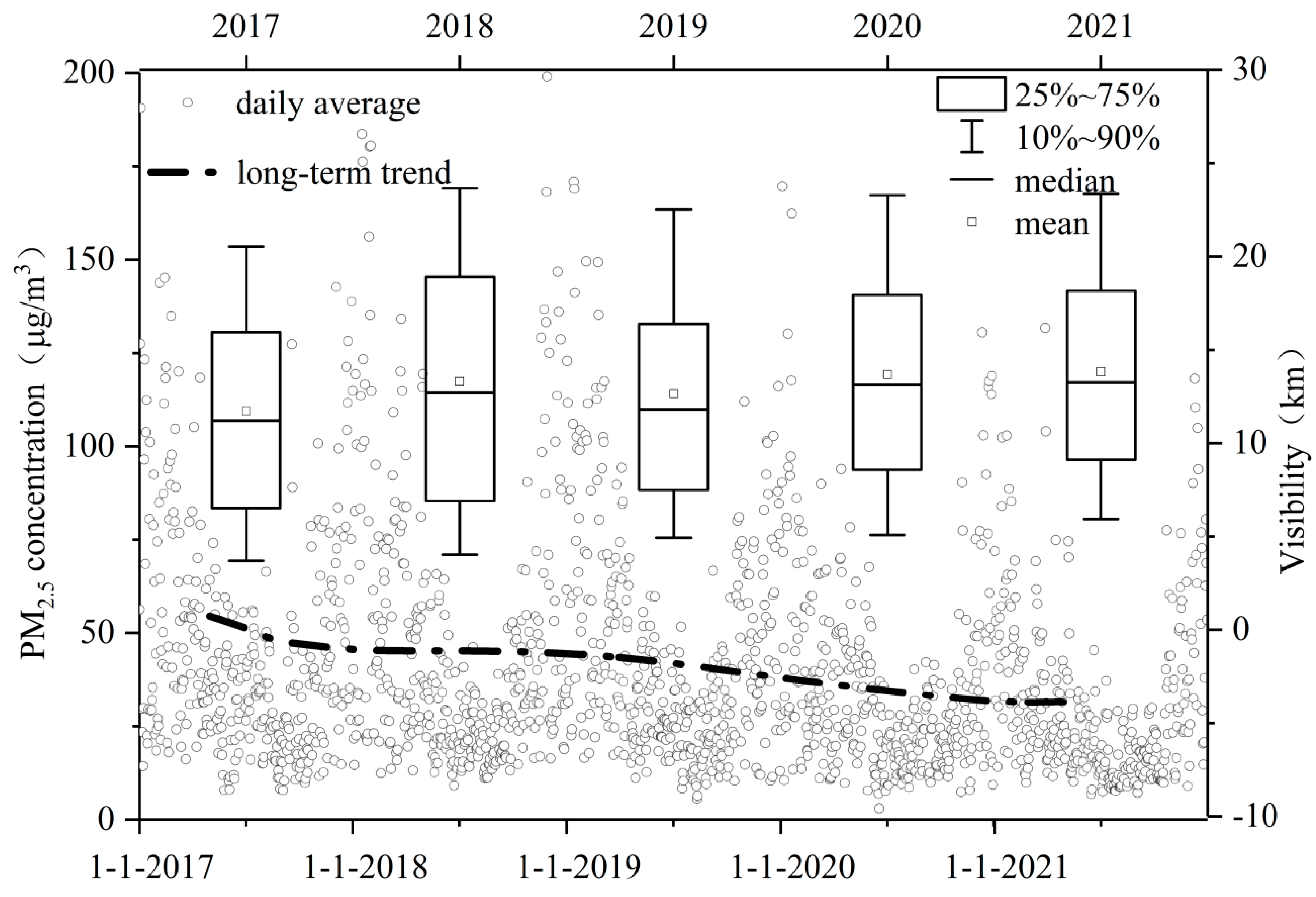
3.1.1. Annual Variation of PM_2.5 Concentration

In order to eliminate the impact of diurnal and seasonal fluctuations, more intuitively obtain the evolution characteristics of PM_2.5. In this study, a KZ(365,3) filter was used to extract the long-term PM_2.5 trend. As shown in Figure 2, the PM_2.5 concentration in Yancheng has shown a decreasing trend in the past five years. From 2017 to 2021, the PM_2.5 mass concentration in Yancheng decreased from 44.79 ± 31.22 μg/m³ in 2017 to 29.66 ± 21.69 μg/m³ in 2021, with a decrease of about 33.8%. It was lower than the annual mean mass concentration of 42 μg/m³ in Beijing, in 2019 [24], and 40 μg/m³ in Jiangsu Province, in 2020 [25,26]. The annual average PM_2.5 mass concentration in Yancheng has been lower than secondary standard of environment air quality GB3095-2012 (35 μg /m³) since 2020, but still higher than the guideline standard of World Health Organization (WHO) (10 μg/m³) [27]. The reduction in PM_2.5 concentration in Yancheng is mainly related to emission reduction measures in China, and the restrictions during the COVID-19 pandemic also has a certain contribution after 2020. The visibility in Yancheng increased from 11.69 ± 6.46 km in 2017 to 13.85 ± 6.24 km 2021, with a cumulative increase of 18.4% in 5 years.

According to Figure 3, the proportion with PM_2.5 daily average mass concentration lower than secondary standard of environment air quality (PM_2.5 daily average mass concentration ≤ 75 μg/m³) is 84.37%, 84.68%, 87.02%, 91.64% and 95.36%, respectively. At the same time, the proportion lower than the primary standard (the daily average mass concentration of PM_2.5 ≤ 35 μg/m³) was 48.86%, 55.43%, 50.83%, 64.84% and 72.75%, respectively. The above data shows that the air quality in Yancheng has gradually improved.

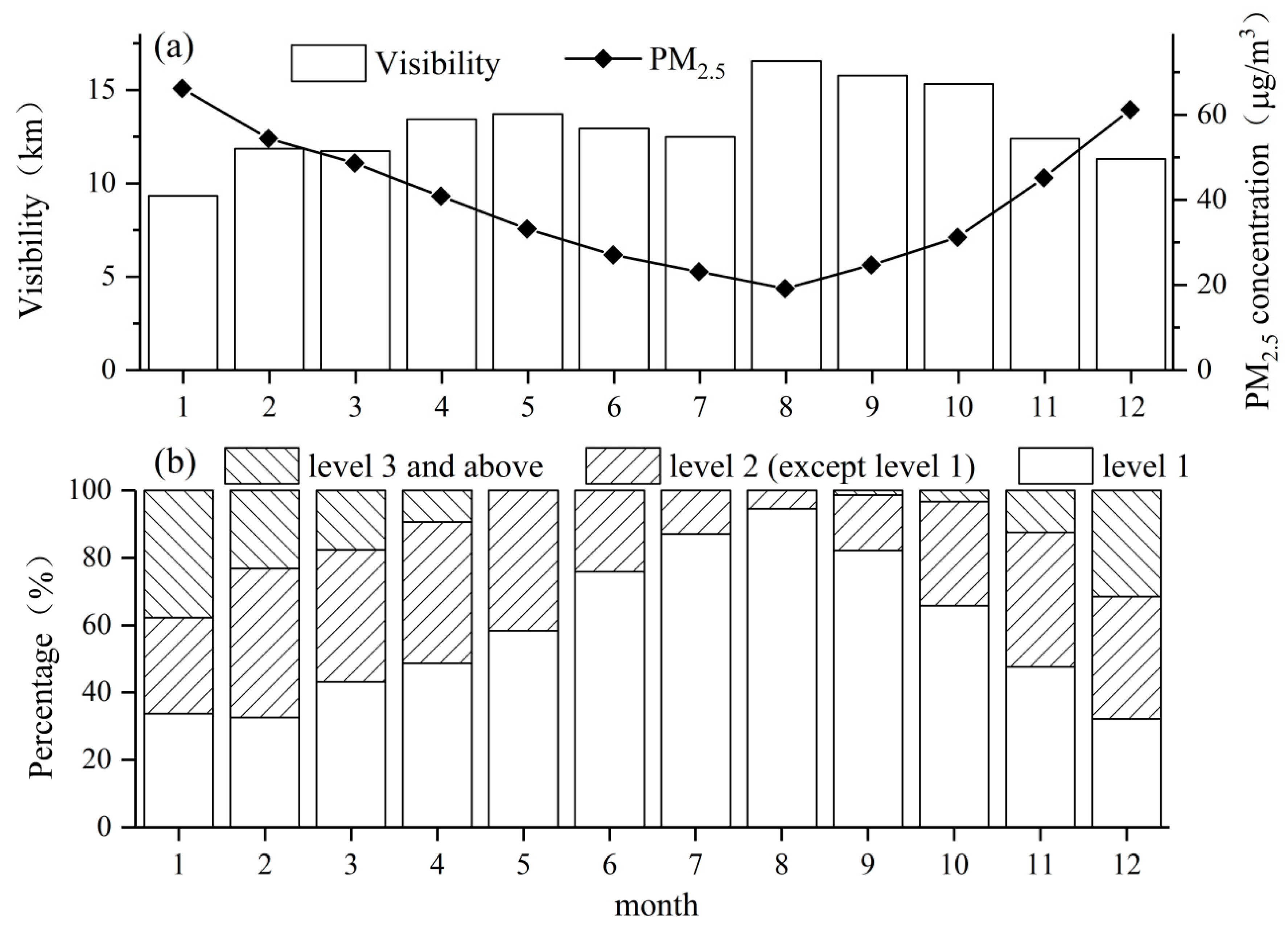
3.1.2. Monthly and Seasonal Variations of PM_2.5

As can be seen from Figure 4a, the monthly average concentration of PM_2.5 shows a unimodal distribution with significant monthly variation. The PM_2.5 concentration was the highest in January (66.19 μg/m³) and the lowest in August (19.17 μg/m³), with the concentration in January being 3.5 times higher than that in August. The variation of atmospheric visibility is opposite to that of PM_2.5 concentration: the highest value occurs in August (16.54 km), and the lowest value occurs in January (9.33 km). The PM_2.5 concentration decreased in June and July, and visibility also decreased slightly. This may be due to the two months that are in the plum rain season, with more precipitation, which is conducive to the wet deposition of pollutants, but at the same time, the precipitation reduces visibility. As can be seen from Figure 4b, the average daily concentration of PM_2.5 in Yancheng from May to August was all lower than the secondary standard of environment air quality, with the lowest proportion (62.3%) in January. The proportion of PM_2.5 daily average concentration lower than the national first standard of environment air quality was the highest in August, reaching 94.6%. Through seasonal discussion, the PM_2.5 concentration in Yancheng has a significant seasonal variation, with the highest in winter (60.61 μg/m³), lowest in summer (23.11 μg/m³), which is consistent with the conclusions of Lu et al. [27] and Jing et al. [20] on the seasonal variation of pollutants in Nanjing. The average visibility in autumn was the highest (14.49 km), slightly higher than that in summer (13.99 km). The visibility was lowest in winter (10.83 km), at only 74.7% of the visibility in summer. The proportion of the PM_2.5 daily average concentration lower than the national second standard of environment air quality in Yancheng was the highest in summer (100%), much higher than that in winter (68.9%).

Yancheng is located in the subtropical monsoon climate zone. Affected by the subtropical anticyclone and the East Asian monsoon in summer, the easterly wind prevails, which can easily transport clean air masses from the sea; high temperature and violent turbulence activity result in strong pollutant diffusion capacity; more precipitation is favorable for wet sedimentation of PM_2.5. Affected by the continual cold high in summer, the westerly wind prevails, which can easily transport polluted air masses from inland; stable atmospheric stratification and a low atmospheric boundary layer are not conducive to the diffusion of pollutants [28,29,30]. The PM_2.5 concentration is the highest in winter and the lowest in summer, so the visibility in summer is higher than that in winter. Through comparative analysis of the precipitation and visibility data of Yancheng, from 2017–2021, it is found that the average visibility with precipitation (7.08 km) is significantly lower than that without precipitation (13.65 km), and precipitation has a significant impact on visibility. The difference in PM_2.5 concentration between autumn and summer in Yancheng is small, but the precipitation in autumn is significantly lower than that in summer. The visibility in autumn is less affected by precipitation, so the visibility in autumn in Yancheng is slightly higher than that in summer.

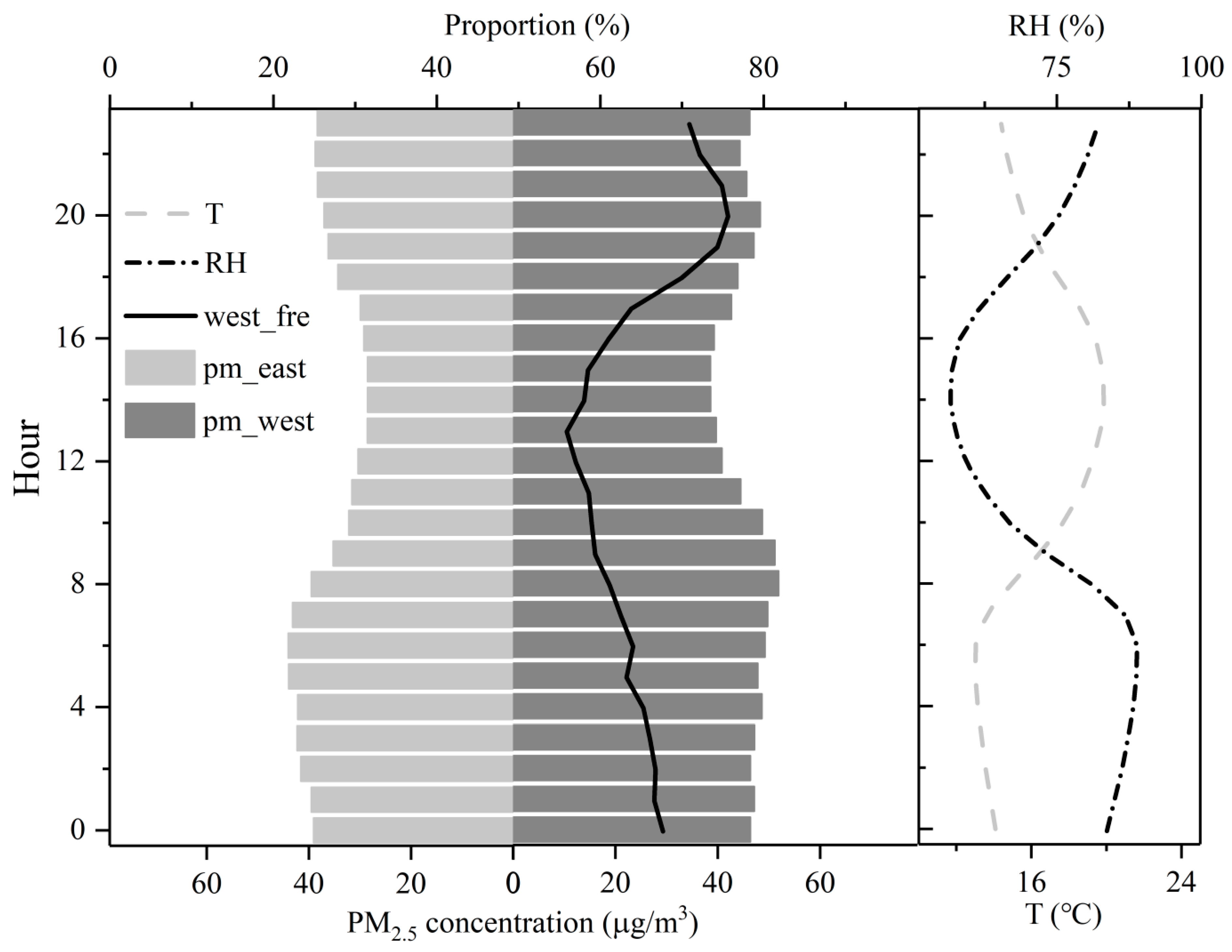
3.1.3. Diurnal Variations of PM_2.5

As can be seen from Figure 5, the diurnal variation of PM_2.5 concentration in Yancheng presents a unimodal distribution. The concentration of PM_2.5 rises slowly from 0 to 6, reaches its peak at around 7 to 8, and then gradually decreases, with the peak value generally appearing at 15. The temperature is the lowest at about 6, the highest at 14–15, and the relative humidity variations are in reverse. Some studies have found that the diurnal variation of urban PM_2.5 concentration is mainly affected by diurnal variation of human activities and meteorological conditions [31,32,33]. After sunset, solar radiation disappears, temperature drops, and relative humidity rises. Inversion stratification gradually forms near the ground, and turbulent activities are inhibited, making it difficult for pollutants to diffuse in the atmosphere. The PM_2.5 accumulates near the ground, resulting in an increase in concentration accumulation [34]. The rush hour is around 7, when the number of motor vehicles on the road increases; the emission of PM_2.5 reaches the maximum during this period, and the concentration peaks at that time. After sunrise, the ground receives solar radiation, the temperature rises, the atmospheric boundary layer continues to rise, and the convection and turbulence become intense, which is conducive to the diffusion of PM_2.5 and reaches the valley value at 14–15.

Yancheng is located in the eastern coastal area of Jiangsu Province, and there are obvious diurnal variations in the direction of sea–land breeze. Generally speaking, 0–8 is the general occurrence period of land wind, 12–20 is the general occurrence period of sea breeze, and the rest is the transition period [35,36], which is consistent with the hourly variation of the proportion of easterly wind in Yancheng in this study. From 2017 to 2021, the PM_2.5 concentration under the easterly wind at Yancheng was 36.60 μg/m³, and the PM_2.5 concentration under the westerly wind was 45.37 μg/m³. The western parts of Yancheng have gradually dense population and developed industries, and the air pollution is more serious; the eastern section of Yancheng is the sea, and the sea breeze has a significant effect on the removal of PM_2.5. The peak–valley difference in PM_2.5 hourly mean concentration corresponding to the easterly wind is greater than that of the westerly wind (15.55 μg/m³ and 13.33 μg/m³), which may be due to the high wind speed in the daytime, and the oceanic air mass corresponding to the easterly wind is relatively clean, and the scavenging effect is more obvious.

3.2. Relationship between PM_2.5 Concentration and Meteorological Elements

3.2.1. Correlation Analysis between PM_2.5 Mass Concentration and Meteorological Elements

In order to explore the correlation characteristics between PM_2.5 concentration and surface meteorological elements in different seasons, this paper conducted a correlation analysis between the hourly mean value of PM_2.5 mass concentration and the hourly value of conventional meteorological elements (visibility, temperature, relative humidity and wind speed) during the period 2017–2021, and the results are shown in

Table 1. Correlation coefficient between PM_2.5 mass concentration and meteorological factors in Yancheng from 2017 to 2021.

	Season	VIS	T	RH	WS
PM2.5 concentration	Spring	−0.52 **	−0.09 **	0.01 **	−0.23 **
	Summer	−0.47 **	0.03	0.01	−0.27 **
	Autumn	−0.52 **	−0.30 **	0.20 **	−0.26 **
	Winter	−0.60 **	0.01	0.22 **	−0.28 **

** pass the 0.01 significance test.

. There is a good correlation between PM_2.5 concentration and visibility and wind speed. The correlation between PM_2.5 concentration and visibility in different seasons is the best, and the correlation coefficient is −0.47 ~ −0.60, showing a strong negative correlation. There is a positive correlation between PM_2.5 concentration and relative humidity in autumn and winter, which may be related to the humidity absorption growth of PM_2.5 particles; the correlation did not pass the test in summer, which may be due to the fact that high humidity conditions in summer mostly occur in precipitation weather, which is conducive to the wet deposition of PM_2.5. Generally speaking, with the increase in temperature, the vertical motion of the atmosphere near the ground is enhanced, and the atmospheric boundary layer is raised, and the vertical motion becomes intense, which is conducive to the diffusion and transmission of PM_2.5. The PM_2.5 concentration and temperature in Yancheng showed a negative correlation in spring and autumn, but failed to pass the test in summer and winter. This may be because the low temperature in summer is usually accompanied by precipitation and strong wind, which is conducive to BC diffusion and wet deposition (i.e., low temperature and low PM_2.5). In winter, under the influence of the cold air in the north, the temperature before the cold front rises, while pollutants accumulate and the concentration of PM_2.5 increases (i.e., high temperature and high PM_2.5). There was a good negative correlation between PM_2.5 concentration and wind speed in different seasons, and the correlation coefficient was −0.23 ~ −0.28. The relationship between wind speed and PM_2.5 concentration also depends on wind direction, which will be further studied later.

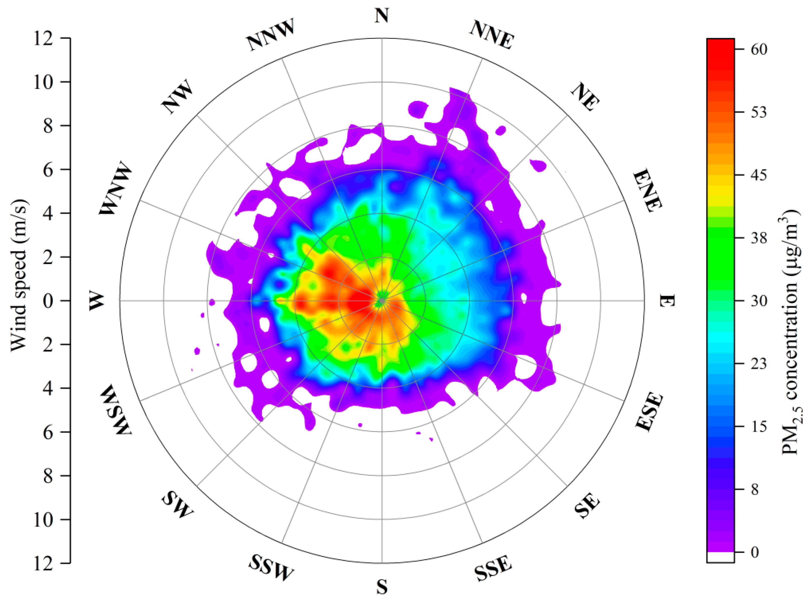
3.2.2. The Relationship between PM_2.5 Concentration and Wind Direction and Wind Speed

Figure 6 illustrates the PM_2.5 concentration under different wind direction and wind speed in Yancheng. In addition to northeast, northeast and northeast directions, high PM_2.5 concentration appeared in Yancheng when the speed was relatively low. The PM_2.5 concentrations are easy to accumulate and difficult to spread when the wind speed is low, which may be caused by the local pollution emission in Yancheng. When the observed wind speed increases, the corresponding PM_2.5 concentration in the direction of northwest–northeast–southwest decreases rapidly, which is mainly because the marine air mass in this direction is relatively clean, and the large near-surface wind speed is conducive to the dilution and diffusion of PM_2.5. The corresponding PM_2.5 concentration in the direction of northwest–southeast–southwest still has a high value when the wind speed is relatively high. The air mass in this direction mainly comes from the inland direction, which is densely populated and industrially developed, and the corresponding air mass is heavily polluted. Therefore, this is mainly related to the transport of the polluted air mass in the inland direction.

3.2.3. The Relationship between PM_2.5 Concentration and Visibility under Different Relative Humidity Conditions

Low visibility is an important cause of road traffic and aircraft takeoff and landing accidents, but also brings serious harm to people’s physical and mental health. Figure 7 reflects the relationship between hourly PM_2.5 concentration and visibility under different relative humidity during the observation period. It can be seen from Figure 7 that the distribution of PM_2.5 concentration and visibility varies greatly under different relative humidity: When the relative humidity is greater than 90%, the corresponding visibility is mostly less than 5 km, and with the decrease in the relative humidity, the visibility on the whole presents a relatively obvious upward trend; low visibility conditions mostly correspond to higher concentration of PM_2.5, but with the increase in relative humidity, even the cleaner atmosphere is prone to obstruction to vision. Therefore, the relative humidity was divided into five sections in this paper, and the PM_2.5 concentration and visibility under different relative humidity sections were fitted. It was found that the two showed a power function relationship, and the results were shown in

Table 2. Quantitative relation between the visibility and PM_2.5 corresponding to different relative humidity ranges.

RH	Fitting Equation	Correlation Coefficient	Threshold (ųg/m3)	Mean VIS (km)	Percentage (%)
RH ≤ 40%	Vis = 59.63x−0.32	−0.78	265	21.33	6.90
40% < RH ≤ 60%	Vis = 63.57x−0.37	−0.74	148	18.98	16.90
60% < RH ≤ 80%	Vis = 64.61x−0.44	−0.64	69	15.52	29.83
80% < RH ≤ 90%	Vis = 50.56x−0.47	−0.57	31	11.35	17.79
RH > 90%	Vis = 22.72x−0.40	−0.41	8	6.44	28.58

. With the increase in relative humidity, the correlation between PM_2.5 concentration and visibility showed a decreasing trend. Under low humidity (<40%), their correlation is the best (−0.78), while under high humidity (>90%), their correlation is the least (−0.41).

According to the division of meteorology, the horizontal visibility of 1–10 km is light fog. Therefore, this paper takes 10km as the visibility threshold and calculates the corresponding PM_2.5 concentration in different relative humidity intervals according to the fitting equation. As can be seen from Table 2, with the increase in relative humidity, the average visibility in the corresponding humidity interval decreases significantly. When the relative humidity is greater than 90%, the corresponding average visibility is only 6.44 km. In addition, with the increase in humidity, the PM_2.5 concentration corresponding to the visibility threshold decreases rapidly; that is, under the condition of high relative humidity, only low PM_2.5 concentration is required to cause obstruction to vision. As a coastal city, Yancheng has a relatively high relative humidity, which reaches 76.2% when the relative humidity exceeds 60%. This is the reason for the frequent occurrence of obstruction to vision in Yancheng under the background of gradual improvement of air quality (visibility below 10km accounted for 53.5% in 2017; 40.8%, 2021).

3.2.4. Potential Source Contribution Function Analysis

In Figure 1a and

Table 3. Trajectory clustering characteristics of Yancheng, from 2017 to 2021.

Cluster	Percentage (%)	Passing Area	PM2.5 Concentration (ųg/m3)
1	30.98	Southwest Jiangsu, Southeast Anhui, northeast Zhejiang	48.0
2	35.40	Yellow Sea, Central Shandong, Tianjin, Beijing, northern Hebei	42.9
3	33.62	Yellow Sea	29.3

, 3D trajectory clustering with a height of 500 m and the passing regions of different clustering trajectories can be obtained, corresponding to the average concentration of PM_2.5. It can be seen that the cluster trajectory of the first type mainly comes from the southwest of Jiangsu, the southeast of Anhui and the northeast of Zhejiang. This region is densely populated and economically developed, which corresponds to the highest PM_2.5 concentration. The second cluster trajectory is mainly from the Yellow Sea, central Shandong, Tianjin, Beijing and northern Hebei, which is also densely populated and economically developed. However, the trajectory passes through the Yellow Sea halfway, and the corresponding PM_2.5 concentration is lower than that of trajectory 1; the third trajectory is mainly from the Yellow Sea, corresponding to the lowest PM_2.5 concentration. Marine air mass contributed little to PM_2.5 pollution in Yancheng, while air mass from land contributed a lot to PM_2.5 transport.

By calculating PM_2.5 concentration under different wind direction and wind speed as well as different cluster trajectories, the main source direction of high concentration PM_2.5 in Yancheng can be preliminarily determined, but the relative contribution of potential source region cannot be specifically determined. In order to further explore the contribution of different regions to PM_2.5 concentration in Yancheng, this section uses PSCF to study the potential sources region. Figure 8 reveals the potential contribution of PM_2.5 from different seasons in Yancheng during the period 2017–2021. On the whole, the seasonal difference in PM_2.5 transport is obvious in Yancheng. The range of high potential source region was wide in autumn and winter, and vice versa in spring and summer. In winter, the PSCF high potential source region (>0.7) in Yancheng is mainly located in southwest Jiangsu, south Anhui and north Jiangxi, which is the main source of PM_2.5 pollution in Yancheng. In addition, southwest Shandong has a great contribution. The high potential source region in autumn was located in the northwest of Zhejiang and the southwest of Jiangsu.

4. Conclusions

The mass concentration of PM_2.5 in Yancheng showed a decreasing trend from 2017 to 2021, with a decline rate of about 33.8% (2017, 44.79 ± 31.22 μg/m³; 2021, 29.66 ± 21.69 μg/m³). In addition to emission reduction measures, the restrictions during the COVID-19 pandemic after 2020 also has a certain contribution. The visibility increased by 18.4% (2017, 11.69 ± 6.46 km; 2021,13.8 ± 6.24 km). The monthly average PM_2.5 concentration was the highest in January (66.19 μg/m³) and the lowest in August (19.17 μg/m³). The diurnal variation of PM_2.5 mass concentration showed a unimodal distribution. The PM_2.5 concentration in Yancheng had a negative correlation with visibility, wind speed and temperature (spring and autumn), and a positive correlation with relative humidity (spring, autumn and winter). A significant attenuation effect of precipitation on visibility (with precipitation, 7.08 km; without precipitation, 13.65 km) is an important reason that the visibility of Yancheng in summer (PM_2.5 concentration is at the valley value) is slightly worse than that in autumn. The correlation between PM_2.5 and visibility increases with the decrease in relative humidity and can be well fitted with a power function. Under the condition of high relative humidity, only a low PM_2.5 concentration is required to cause obstruction to vision. The sea breeze has obvious scavenging effect on PM_2.5 (easterly wind, 36.60 μg/m³; westerly wind, 45.37 μg/m³). The high concentration of PM_2.5 in Yancheng mainly comes from the direction of northwest–southeast–southwest. After clustering the backward trajectories, it is found that the air masses passing through the sea are obviously cleaner, and the air masses coming from inland are more likely to cause the high concentration of PM_2.5 in Yancheng. According to PSCF, the potential source regions in autumn are mainly distributed in southwestern Jiangsu and northwestern Zhejiang; the potential source regions in winter are mainly located in southwestern Jiangsu, southern Anhui and northern Jiangxi.

References

1. Liu, L.; Hu, F. Multi-attribute decision-based multi-objective optimization for regional atmospheric compound pollution control. Clim. Environ. Res. 2019, 24, 407–416. (In Chinese) [Google Scholar] [CrossRef]
2. Feng, Y.; Huang, X.; Sun, H.; Liu, C.; Zhang, B.; Zhang, Z.; Tengur, V.S.; Chen, W.; Wu, T.; Yuan, J.; et al. Framingham risk score modifies the effect of PM10 on heart rate variability. Sci. Total Environ. 2015, 523, 146–151. [Google Scholar] [CrossRef] [PubMed]
3. Deng, X.; Tie, X.; Wu, D.; Zhou, X.; Bi, X.; Tan, H.; Li, F.; Jiang, C. Long-term trend of visibility and its characterizations in the Pearl River Delta (PRD) region, China. Atmos. Environ. 2008, 42, 1424–1435. [Google Scholar] [CrossRef]
4. Ma, Z.W.; Hu, X.F.; Sayer, A.M.; Levy, R.; Zhang, Q.; Xue, Y.; Tong, S.; Bi, J.; Huang, L.; Liu, Y. Satellite-based spatiotemporal trends in PM2.5 concentrations: China, 2004–2013. Environ. Health Perspect. 2016, 124, 184–192. [Google Scholar] [CrossRef] [PubMed]
5. Hong, T.; Shakya, A.; Feng, W.; Wu, W.; Wei, L. Comparative ligandomic analysis of human lung epithelial cells exposed to PM2.5. Biomed. Environ. Sci. 2020, 33, 165–173. [Google Scholar]
6. Hu, Z.M.; Wang, J.; Tao, Z.; Chen, Z. Pollution level and health risk assessment of heavy metals in PM2.5, Shanghai. Acta Sci. Circumstantiae 2013, 12, 3399–3406. [Google Scholar]
7. Hou, X.; Zhu, B.; Kumar, K.R.; Lu, W. Inter-annual variability in fine particulate matter pollution over China during 2013–2018: Role of meteorology. Atmos. Environ. 2019, 214, 116842. [Google Scholar] [CrossRef]
8. Huang, X.; Tang, G.; Zhang, J.; Liu, B.; Liu, C.; Zhang, J.; Cong, L.; Cheng, M.; Yan, G.; Gao, W.; et al. Characteristics of PM2.5 pollution in Beijing after the improvement of air quality. J. Environ. Sci. 2021, 100, 1–10. [Google Scholar] [CrossRef]
9. Ji, D.; Yan, Y.; Wang, Z.; He, J.; Liu, B.; Sun, Y.; Gao, M.; Li, Y.; Cao, W.; Cui, Y.; et al. Two-year continuous measurements of carbonaceous aerosols in urban Beijing, China: Temporal variations, characteristics and source analyses. Chemosphere 2018, 200, 191–200. [Google Scholar] [CrossRef]
10. Jacob, D.J.; Darrell, A.W. Effect of climate change on air quality. Atmos. Environ. 2009, 43, 51–63. [Google Scholar] [CrossRef]
11. Zhang, R.H.; Li, Q.; Zhang, R.N. Meteorological conditions for the persistent severe fog and haze event over eastern China in January 2013. Sci. China Earth Sci. 2014, 57, 26–35. [Google Scholar] [CrossRef]
12. Cheng, Y.F.; Hou, X.W.; Zhu, B.; Lu, W. The meteorological causes of a heavy pollution process in BTH and YRD area with stable weather condition. Acta Sci. Circumstantiae 2020, 40, 1575–1586. [Google Scholar]
13. Chen, Y.N.; Luo, L.; Ma, H.; Jia, Y.; Zhao, J.; Xu, C.; Lou, X.; Yu, Y. Construction and application of stable weather index in Hangzhou. Acta Sci. Circumstantiae 2020, 12, 4461–4469. [Google Scholar]
14. Zhang, H.D.; Lü, M.Y.; Zhang, B.H. Analysis of the stagnant meteorological situation and the transmission condition of continuous heavy pollution course from February 20 to 26, 2014 in Beijing-Tianjin-Hebei. Acta Sci. Circumstantiae 2016, 36, 4340–4351. [Google Scholar]
15. Wang, Y.; Xuan, W.; Kondo, Y.; Kajino, M.; Munger, J.W.; Hao, J. Black carbon and its correlation with trace gases at a rural site in Beijing: Top-down constraints from ambient measurements on bottom-up emissions. J. Geophys. Res. Atmos. 2011, 116. [Google Scholar] [CrossRef]
16. Wang, L.J.; Liu, X.H.; Lu, W.; Zhang, C.; Tang, W.Y.; Zhu, B. Impact of a cold front transport process on haze weather in eastern China in early winter. China Environ. Sci. 2021, 41, 2004–2013. [Google Scholar] [CrossRef]
17. Wang, H.L.; Qiao, L.P.; Lou, S.R.; Zhou, M.; Ding, A.J.; Huang, H.Y.; Chen, J.M.; Wang, Q.; Tao, S.K.; Chen, C.H.; et al. Chemical composition of PM2.5 and meteorological impact among three years in urban Shanghai, China. J. Clean. Prod. 2016, 112, 1302–1311. [Google Scholar] [CrossRef]
18. Rao, S.T.; Zurbenko, I.G.; Neagu, R.; Porter, P.S.; Ku, J.Y.; Henry, R.F. Space and Time Scales in Ambient Ozone Data. Bull. Am. Meteorol. Soc. 1997, 78, 2153–2166. [Google Scholar] [CrossRef]
19. Kang, H.; Zhu, B.; de Leeuw, G.; Hou, C.; Gao, J. Natural and anthropogenic contributions to long-term variations of SO2, NO2, CO, and AOD over East China. Atmos. Res. 2018, 215, 284–293. [Google Scholar] [CrossRef]
20. Jing, A.; Zhu, B.; Wang, H.; Yu, X.; An, J.; Kang, H. Source apportionment of black carbon in different seasons in the northern suburb of Nanjing, China. Atmos. Environ. 2019, 201, 190–200. [Google Scholar] [CrossRef]
21. Liu, A.K.; Wang, H.L.; Cui, Y.; Shen, L.; Yin, Y.; Wu, Z.; Guo, S.; Shi, S.; Chen, K.; Zhu, B.; et al. Characteristics of Aerosol during a Severe Haze-Fog Episode in the Yangtze River Delta: Particle Size Distribution, Chemical Composition, and Optical Properties. Atmosphere 2020, 11, 56. [Google Scholar] [CrossRef]
22. Cao, J.J.; Xu, B.Q.; He, J.Q.; Liu, X.-Q.; Han, Y.-M.; Wang, G.-H.; Zhu, C.-S. Concentrations, seasonal variations, and transport of carbonaceous aerosols at a remote Mountainous region in western China. Atmos. Environ. 2009, 43, 4444–4452. [Google Scholar] [CrossRef]
23. Dai, M.; Zhu, B.; Fang, C.; Zhou, S.; Lu, W.; Zhao, D.; Ding, D.; Pan, C.; Liao, H. Long-Term Variation and Source Apportionment of Black Carbon at Mt. Waliguan, China. J. Geophys. Res. Atmos. 2021, 126, e2021JD035273. [Google Scholar] [CrossRef]
24. Zhang, M. Numerical Study on Transport Characteristics of PM2.5 under Different Pollution Conditions in Beijing during Wintertime. Plateau Meteorol. 2022, 41, 829–838. [Google Scholar] [CrossRef]
25. Wu, K.; Meng, Y.; Gong, Y.; Zhang, X.; Wu, L.; Ding, X.; Chen, X. Surveillance of long-term environmental elements and PM2.5 health risk assessment in Yangtze River Delta, China, from 2016 to 2020. Environ. Sci. Pollut. Res. 2022, 29, 81993–82005. [Google Scholar] [CrossRef] [PubMed]
26. Yin, C.; He, J.; Yu, L.; Jiao, Y.; Zhou, L. The impact of multi-scale meteorological conditions on PM2.5 pollution over Ji’nan. Plateau Meteorol. 2019, 38, 1120–1128. [Google Scholar] [CrossRef]
27. Lu, W.; Wang, H.L.; Zhu, B.; Shi, S.; Kang, H. Distribution characteristics of PM2.5 mass concentration and their impacting factors including meteorology and transmission in North Suburb of Nanjing during 2014 to 2016. Acta Sci. Circumstantiae 2019, 39, 1039–1048. [Google Scholar]
28. Chen, L.W.A.; Doddridge, B.G.; Dickerson, R.R.; Chow, J.C.; Mueller, P.K.; Quinn, J.; Butler, W.A. Seasonal variations in elemental carbon aerosol, carbon monoxide and sulfur dioxide: Implications for sources. Geophys. Res. Lett. 2001, 28, 1711–1714. [Google Scholar] [CrossRef]
29. Ji, D.; Li, L.; Pang, B.; Xue, P.; Wang, L.; Wu, Y.; Zhang, H.; Wang, Y. Characterization of black carbon in an urban-rural fringe area of Beijing. Environ. Pollut. 2017, 223, 524–534. [Google Scholar] [CrossRef]
30. Dan, M.; Zhuang, G.; Li, X.; Tao, H.; Zhuang, Y. The characteristics of carbonaceous species and their sources in PM2.5 in Beijing. Atmos. Environ. 2004, 38, 3443–3452. [Google Scholar] [CrossRef]
31. Arif, M.; Kumar, R.; Kumar, R.; Eric, Z.; Gourav, P. Ambient black carbon, PM2.5 and PM10 at Patna: Influence of anthropogenic emissions and brick kilns. Sci. Total Environ. 2018, 624, 1387–1400. [Google Scholar] [CrossRef] [PubMed]
32. Cao, J.J.; Zhu, C.S.; Chow, J.C.; Watson, J.G.; Han, Y.-M.; Wang, G.-H.; Shen, Z.-X.; An, Z.-S. Black carbon relationships with emissions and meteorology in Xi’an, China. Atmos. Res. 2009, 94, 194–202. [Google Scholar] [CrossRef]
33. Rajesh, T.A.; Ramachandran, S. Characteristics and source apportionment of black carbon aerosols over an urban site. Environ. Sci. Pollut. Res. Int. 2017, 24, 8411. [Google Scholar] [CrossRef] [PubMed]
34. Trompetter, W.J.; Grange, S.K.; Davy, P.K.; Ancelet, T. Vertical and temporal variations of black carbon in New Zealand urban areas during winter. Atmos. Environ. 2013, 75, 179–187. [Google Scholar] [CrossRef]
35. Wang, J.; Zhao, L.J. The characteristics of sea-land breeze circulation and the influence of ambient air quality in Xiamen. Environ. Sci. 2017, 42, 30–33. [Google Scholar]
36. Boucouvala, D.; Bornstein, R. Analysis of transport patterns during an SCOS97-NARSTO episode. Atmos. Environ. 2003, 37, 73–94. [Google Scholar] [CrossRef]
Figure 1. Schematic diagram of the observation point (a) is the 3D trajectory clustering of 500 m height during the observation period, where the white, yellow and red line segments are trajectories 1, 2 and 3, respectively; (b) is the schematic diagram of geographical location of sampling points).
Atmosphere 14 00317 g001
Figure 2. Time series of PM2.5 and visibility from 2017 to 2021. The hollow circle is the daily average concentration of PM2.5. The dashes are the long-term trend of PM2.5 after KZ filtering. Boxplots show the interannual variation of visibility; the top and bottom short lines indicate 10% and 90% quantiles. The rectangle represents the 25% and 75% quantiles, and the inner short line of the rectangle is the median.
Atmosphere 14 00317 g002
Figure 3. The proportion of days of different levels of environmental air quality during the period 2017–2021.
Atmosphere 14 00317 g003
Figure 4. Monthly variation of PM2.5 and visibility (a) and proportion of air quality levels in different months (b).
Atmosphere 14 00317 g004
Figure 5. Hourly changes in PM2.5 average concentration, easterly proportion, temperature and relative humidity under different wind directions in Yancheng. The dark gray and light gray bar charts, respectively, show the hourly average PM2.5 concentration in Yancheng under easterly and westerly winds. The solid black line shows the proportion of easterly winds in Yancheng, the gray dashed line is the temperature, and the black dashed line is the relative humidity.
Atmosphere 14 00317 g005
Figure 6. PM2.5 concentration under different wind speed and direction.
Atmosphere 14 00317 g006
Figure 7. The relation between the visibility and PM2.5 concentration corresponding to different relative humidity ranges.
Atmosphere 14 00317 g007
Figure 8. The distribution of the potential source contribution function (PSCF) on Yancheng during different season ((a). Spring; (b). Summer; (c). Autumn; (d). Winter).
Atmosphere 14 00317 g008