Article

Simulation Analyses on a Downburst Event That Caused a Severe Tower Toppling down Accident in Zhejiang (China)

1
Transmission & Transformation Engineering Department, China Electric Power Research Institute, Beijing 100055, China
2
Department of Operation & Maintenance, State Grid Corporation of China, Beijing 100031, China
3
China Electric Power Research Institute, Beijing 100055, China
4
State Grid Hunan Electric Power Co., Ltd., Loudi Power Supply Branch, Loudi 417000, China
5
University of Chinese Academy of Sciences, Beijing 100049, China
6
Institute of Atmospheric Physics, Chinese Academy of Sciences, Beijing 100029, China
*
Authors to whom correspondence should be addressed.
Atmosphere 2023, 14(3), 427; https://doi.org/10.3390/atmos14030427
Submission received: 21 January 2023 / Revised: 13 February 2023 / Accepted: 16 February 2023 / Published: 21 February 2023
(This article belongs to the Section Meteorology)

Abstract

:
The downburst events have been a research focus for decades, as their associated disastrously strong winds pose a great threat to aviation, the shipping industry, agriculture, and the power industry. On 14 May 2021, a series of severe convection occurred in middle and eastern China, during which six 500-kilovolt transmission line towers in Zhejiang were toppled down by a downburst event, resulting in a large range of power outages. By using the Weather Research and Forecasting (WRF) model version 4.4, key features of the downburst event were reproduced reasonably; based on which, we explored the evolutionary mechanisms and the three-dimensional structures of the strong winds associated with the downburst event. It was found that a southwest–northeast-orientated, eastward moving strong squall line was the parent convection system for the downburst event. The downburst-associated convection was deep (from surface to 200 hPa); in the near surface layer, it was mainly associated with positive geopotential height and negative temperature deviations, whereas, at higher levels, it was mainly associated with negative geopotential height and positive temperature deviations. Backward trajectory analysis indicates that the air particles that came from the middle troposphere west of the key region (~61.2% in proportion) were crucial for producing the strong winds of the downburst event. These air particles experienced notable descending processes, during which most of the air particles decreased notably in their potential temperature, while they increased significantly in their specific humidity. The kinetic energy budget analyses denote that, for the region surrounding the location where the tower toppling appeared, the work done by the strong pressure gradient force between the high-pressure closed center (corresponding to intense descending motions) and the low-pressure closed center (corresponding to strong latent heat release) dominated the rapid wind enhancement.

1. Introduction

According to the definition from the American Meteorological Society (AMS), the downburst is defined as an area of strong (usually >17.2 m s−1) [1], often damaging, winds produced by one or more convective downdrafts [2]. According to the horizontal scale, Fujita [3] classified the downbursts into two types: the downbursts over horizontal spatial scales ≤4 km are referred to as microbursts, and those events with horizontal spatial scales >4 km are termed macrobursts. Downburst has a significant impact on the aviation and the shipping industry. For example, on 24 June 1975, when a Boeing aircraft was about to land at Kennedy Airport in New York, it encountered a downburst and crashed rapidly, resulting in 113 deaths and 11 injuries [4]. On 1 June 2015, a cruise ship named “Dongfangzhixing” encountered a downburst in the Jianli (Hubei Province) section of the Yangtze River and capsized instantaneously. Up to 442 people were killed in this accident [1,5]. Moreover, the disastrously strong winds associated with downbursts often caused considerable damages to crops, trees, houses, and transmission line towers, resulting in serious casualties and property losses [6,7,8,9,10,11,12,13], Of these, damages to the power facilities were usually more serious as in addition to affecting local regions, downbursts could also affect other regions through causing an interruption to the power supply [7,14,15,16].
Due to their high frequency and strong destructive power [1,13], the downbursts have been a hot research topic for decades. Of these, to understand their formation mechanisms and to explore their three-dimensional (3D) structures are of particular importance. As the downburst events are small in spatial scale and short in temporal scale, high resolution simulations are a useful tool for related studies. For example, Lin [17] used a 3D sub-cloud idealized simulation to reproduce the microbursts and found that the simulation could capture the key features that were observed in real downburst events. Based on the combined Rankine vortex model, Bech et al. [18] developed a methodology that could distinguish microbursts from tornadic events using surface damage. Vermeire et al. [19] used the large eddy simulations to simulate downburst events and found that the maximum horizontal wind was associated with smaller scale structures in the flow caused by the downdraft interactions aloft. Bolgiani et al. [10] applied a series of simulations to determine the best microphysics and planetary boundary layer schemes for simulating the downdrafts associated with severe convections. They found that the high-reflectivity microbursts reproduced by the optimal model configuration were notably consistent with the observations. Although the previous simulation studies had enhanced our understandings of the downburst events, there still remain some unsolved scientific questions about downbursts’ formation and structure. These include evolutionary mechanisms of their kinetic energy and their 3D airflow structure.
In the mid May 2021, a series of severe convective weather events occurred from west to east, with their strongest influencings appearing in central and eastern China. Of these, an intense downburst event occurred on 14 May 2021 in Zhejiang (Figure 1a). During this event, power facilities within Zhejiang suffered heavy losses [16], where six 500-kilovolt (kV) transmission line towers toppled down, resulting in a large range of power outages. The 500 kV transmission line belongs to a high-voltage transmission line, which undertakes the important task of transmitting and distributing electric energy in the power system and plays an important role in ensuring the normal operation of the State Grid [20]. According to the field survey, directions of trees’ dumping at the disaster site showed obvious divergent characteristics, and the instantaneous maximum wind speed might have exceeded 50 m s−1 [16]. All these were typical features of the downbursts associated with severe convections [9,10,11]. Another notable feature for this event was that heavy rainfall appeared simultaneously with the downburst. As Fujita [3] reported, downbursts could be classified into dry downbursts and wet downbursts, according to the precipitation and radar reflectivity associated with them. The wet downbursts usually possess heavier precipitation and more intense radar reflectivity than those of dry downbursts, mainly due to their more abundant moisture condition [21,22]. Based on the previous studies of downbursts, the primary purpose of this study is to reproduce the strong downburst event on 14 May 2021 in Zhejiang, to understand its formation in terms of the kinetic energy budget, and to clarify its 3D airflow structure.
The reminder of this article is structured as follows: Section 2 describes the data, model configuration, and methods used in this study; Section 3 shows the validation of the simulation; Section 4 presents the synoptic analysis on the event; Section 5 shows the 3D structure and the evolutionary mechanisms of the downburst event; and finally a conclusion and discussion is provided in Section 6.

2. Data, Model Configuration, and Methods

2.1. Data

In this study, we used a total of three types of data: (i) the hourly, 0.25° × 0.25° ERA5 reanalysis data from the European Centre for Medium-Range Weather Forecasts (ECMWF) [23] was used for generating the initial and boundary conditions of the numerical simulation, and it was also used for the validation of the simulations of the downburst event’s background environment. This is because the ERA5 reanalysis data showed an overall better performance in China compared to other types of reanalysis data [24,25,26,27]. (ii) The half-hourly GPM IMERG Final Precipitation data [28] was used for the validation of the precipitation simulation. (iii) The 6 min, 1 km × 1 km composite radar reflectivity from the China Meteorological Administration was used for the validation of the convection simulation.

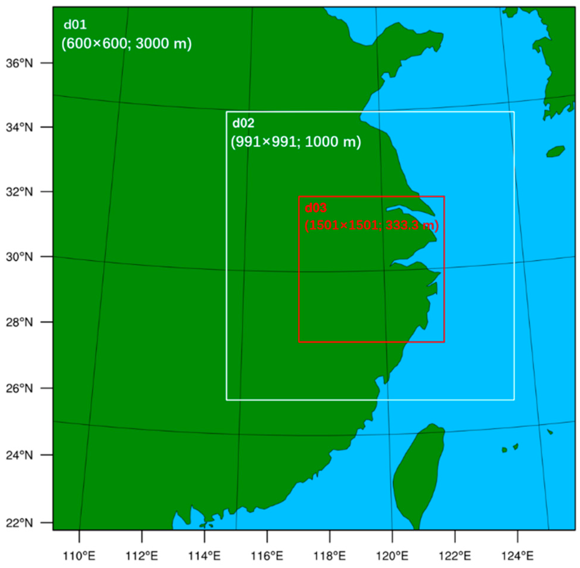
2.2. Model Configuration

In this study, we used the Weather Research and Forecasting (WRF) model v4.4 [29] for the simulation. As shown in Figure 2, a total of three domains (one way nesting) was used, which had 600 × 600, 991 × 991, and 1501 × 1501 grids, respectively. The grid spacings for d01–d03 are 3000 m, 1000 m, and 333.3 m, respectively. As the downburst event appeared in Zhejiang province, which is adjacent to the sea in the east, in order to include the effects from the sea breeze [30], all three domains contain a sea region (Figure 2). In the vertical direction, 51 terrain-following levels were used with the top level fixed at 50 hPa. The physical schemes used in the simulation are listed as follows: the five-layer thermal diffusion land surface model (NOAH) [31]; the Yonsei University planetary boundary layer scheme (YSU) [32]; the old MM5 surface layer scheme [29]; the WRF single-moment 6-class scheme (WSM6) [33]; the Dudhia shortwave scheme [34]; and the rapid radiative transfer model with GCM applications scheme (RRTM) [35]. Of these, the YSU scheme was also proven to be useful for the simulations in North China [36] and East Siberia [37]. No cumulus schemes were used in this study; as all the grid spacings were convection permitting. The simulation was initiated at 06:00:00 UTC 14 May 2021 and ran for 12 h to cover the whole downburst event. The boundary conditions were updated every 3 h during the simulation.

2.3. Kinetic Energy Budget

As an effective indicator for wind speed [38,39,40], the kinetic energy (KE) budget was used in this study to understand the formation of the strong winds associated with the downburst event. The momentum equation under the Cartesian coordinate [41,42] can be written as:
u t + u u x + v u y + w u z = 1 ρ p x + f v + F u ,
v t + u v x + v v y + w v z = 1 ρ p y f u + F v ,
where u, v, and w are the zonal, meridional, and vertical wind in the Cartesian coordinate, respectively; t is the time; z is the height; p is the pressure; and f is the Coriolis parameter. Fu and Fv are the friction force in the x and y directions, respectively. Calculating u ∗ Equation (1) + v ∗ Equation (2), we can obtain Equation (3), as the following shows:
u 2 2 t + u u 2 2 x + v u 2 2 y + w u 2 2 z + v 2 2 t + u v 2 2 x + v v 2 2 y + w v 2 2 z = 1 ρ p x u 1 ρ p y v + u F u + v F v .
Define k h = ( u 2 + v 2 ) / 2 , and then Equation (3) can be rewritten as:
k h t = u k h x + v k h y w k h z 1 ρ p x u 1 ρ p y v + u F u + v F v ,
where k h t denotes the local temporal variation in KE; u k h x + v k h y represents the horizontal advection of KE (HAK); w k h z is the vertical advection of KE (VAK); 1 ρ p x u 1 ρ p y v stands for the work of the pressure gradient force (WOP); and u F u + v F v is the work of the friction force. In order to represent the sum of all terms on the right-hand side of Equation (4), except for the friction force’s work, a sum term (SUM) was defined as SUM = HAK + VAK + WOP. The balance of the KE budget can be represented by the ratio of k h t and SUM [43,44]; a ratio closer to 1.0 means a better balance of the budget (a mean ratio of 0.76 was found for the KE budget equation in this study, implying that the KE budget equation was reasonably balanced after neglecting the friction [45,46].

3. Simulation Validation

According to Wang et al. [16], the downburst event that toppled six 500 kV transmission line towers occurred around 14:12:00 UTC 14 May 2021. Figure 3 illustrates the background environment ~1 h before the event. It is shown that the simulation had reproduced the 200 hPa jet stream well (the correlation between the wind speed of the upper-level jet derived from ERA5 and the simulation was ~0.74). For the middle troposphere, the geopotential height derived from ERA5 and simulation showed a correlation coefficient of ~0.83, and the correlation coefficient of the temperature was ~0.61. A comparison of the sounding (~2 h before the downburst event) at the location where the transmission line towers toppling appeared shows that the simulation had reproduced the inversion layer in the near-surface layer (Figure 4), and the profiles of the temperature and dew point were both well simulated. The strong vertical wind shear at the layer from 1000 hPa to 850 hPa and the wind intensity in the whole layer were both reasonably reproduced. Key parameters such as the lifted condensation level, the pressure of the lifted condensation level, the showalter index, the precipitable water, and the convective availabe potenrial energy (CAPE) were all simulated reasonably. As discussed above, the simulation had captured the key features of the background environment of this event.
As Figure 5a shows, strong rainfall (3 h accumulated precipitation ≥20 mm) appeared northwest of the location where the transmission line towers’ toppling appeared. The simulation reproduced the strong precipitation, but for a stronger intensity (Figure 5b). We calculated the threat score (TS) [47] and found that the TS for the heavy rainfall (i.e., 3 h accumulated precipitation ≥20 mm) simulation was ~0.45. This indicates that the rainfall simulation was reasonable. For the composite radar reflectivity, at 13:44:00 UTC 14 May 2021 (~28 min earlier than the observation), the simulation had reproduced the southwest–northeast-orientated strong reflectivity band (blue tilted dashed box in Figure 1), which directly accounted for the formation of the downburst event. In addition, the strong reflectivity center east of the strong reflectivity band was also reproduced reasonably. The abovementioned indicates that the simulation had captured the key features of the mesoscale systems during the downburst event. Therefore, the simulation of this study can be used for further analysis.

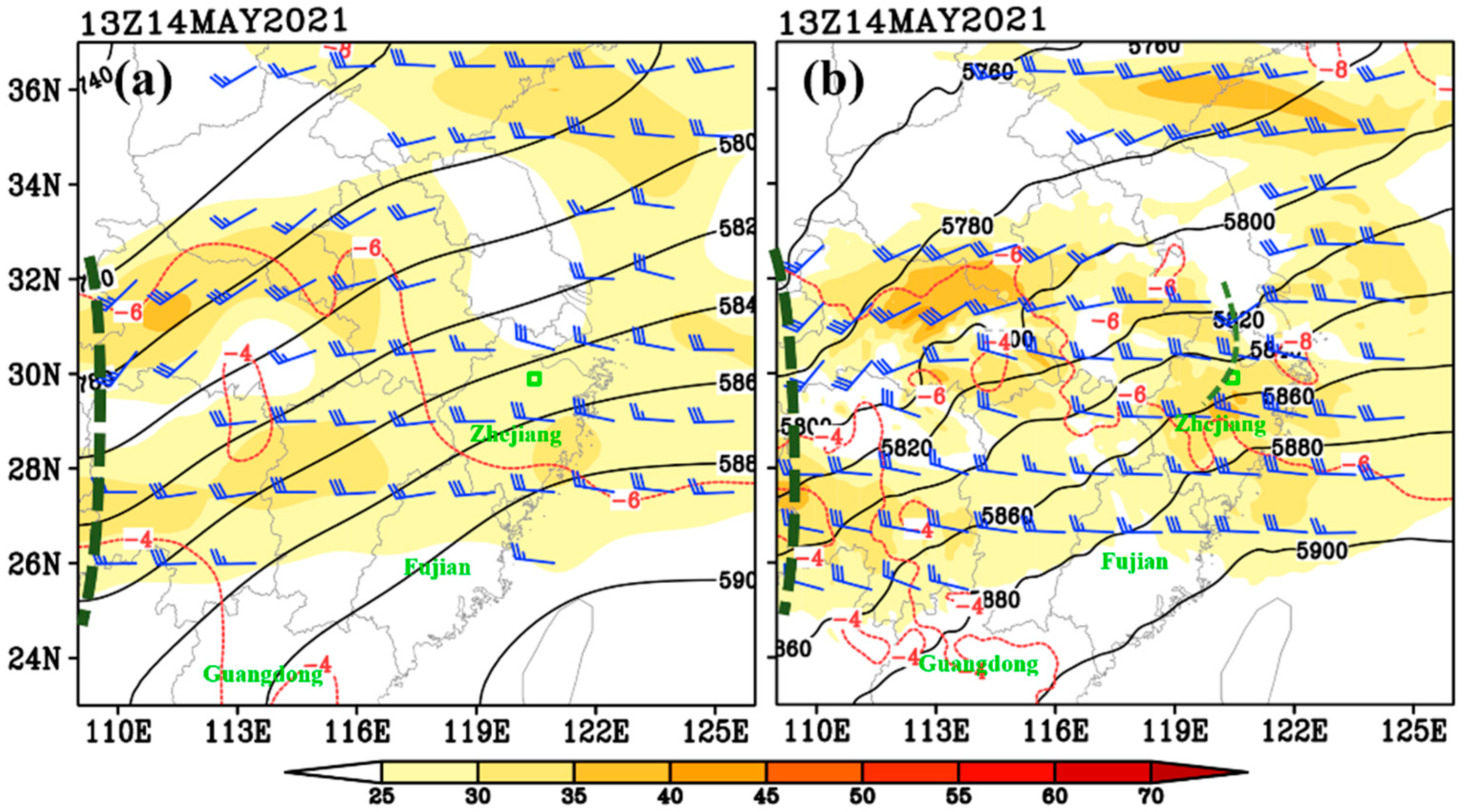
4. Synoptic Analyses

The large-scale background environment of this event was characterized by an intense upper-level jet within the band of 26–32° N (Figure 3b) and a strong Western Pacific subtropical high, of which the 5880 isohypse covered most of Guangdong and Fujian. The former contributed to maintain an upper-level divergence over northern Zhejiang, and the latter favored the northeastward moisture transport into Zhejiang. The location where the transmission line towers toppling appeared was situated within the trough region of a middle-level shortwave trough (Figure 3b), where the quasi-geostrophic forcings favored ascending motions [42]. The sounding ~2 h before the downburst event (at the location where the transmission line towers toppling appeared) featured a lower lifted condensation level, an abundant precipitable water, a large showalter index, a positive CAPE, and a strong near-surface vertical wind shear (Figure 4a), all of which indicate that the conditions were favorable for severe convections.
The simulation indicates that the squall line we focused on in this study formed around 09:00:00 UTC 14 May 2021 (not shown). At 12:04:00 UTC, it had reached its maximum intensity, which could be reflected by a southwest–northeast-orientated band of strong composite radar reflectivity (as Figure 6a shows, the maximum reflectivity was above 70 dBZ). A notable divergent surface wind field was coupled with the strong reflectivity band, with the maximum wind exceeding 17.2 m s−1 (the threshold of a downburst event). Meanwhile, an isolated strong reflectivity center maintained to the southeast of the strong reflectivity band mentioned above. Strong easterly wind and southeasterly wind at the surface appeared within this strong reflectivity center. Around 20 min later, the southwest–northeast-orientated strong reflectivity band moved eastward, during which its southern section strengthened in intensity and enlarged in area, whereas its northern section weakened in intensity rapidly. Correspondingly, the divergent surface wind field associated with the southern section still retained a strong intensity, whereas that of the northern section weakened remarkably (Figure 6b).
From 12:44:00 UTC to 13:04:00 UTC, 14 May 2021, the southwest–northeast-orientated strong reflectivity band moved eastward, where its southern/northern section enhanced/weakened in intensity notably (Figure 6c,d). As Figure 7a,b show, the surface wind speed beneath the strong reflectivity band enhanced rapidly from 12:44:00 UTC to 13:04:00 UTC, particularly for the northwesterly wind, which reached a speed of ≥20 m s−1. The strong surface wind was associated with intense surface divergence (Figure 8a,b), which is a key characteristic of a downburst (the whole event lasted for ~30 min). In contrast, the isolated strong reflectivity center east of the southwest–northeast-orientated strong reflectivity band mainly kept its intensity (Figure 6c,d), with its associated surface wind and divergence changed slowly (Figure 7a,b and Figure 8a,b). The easterly surface wind beneath the isolated strong reflectivity center encountered the northwesterly surface wind beneath the southwest–northeast-orientated strong reflectivity band, which favored the generation of a new convection between the two systems mentioned above.

5. Downburst Event That Caused the Accident

The period from 13:24:00 UTC to 13:44:00 UTC was crucial for the downburst event that caused the transmission line towers toppling down accident in Zhejiang, and thus it was investigated in detail. A key region which covered the main range of the strong winds associated with the downburst event was determined as the purple dashed box in Figure 7d shows. It was used to analyze the horizontal structural features of the downburst event. The longitudes that crossed the surface wind maxima (blue dashed lines in Figure 7d) were determined to analyze the vertical structure of the downburst event.

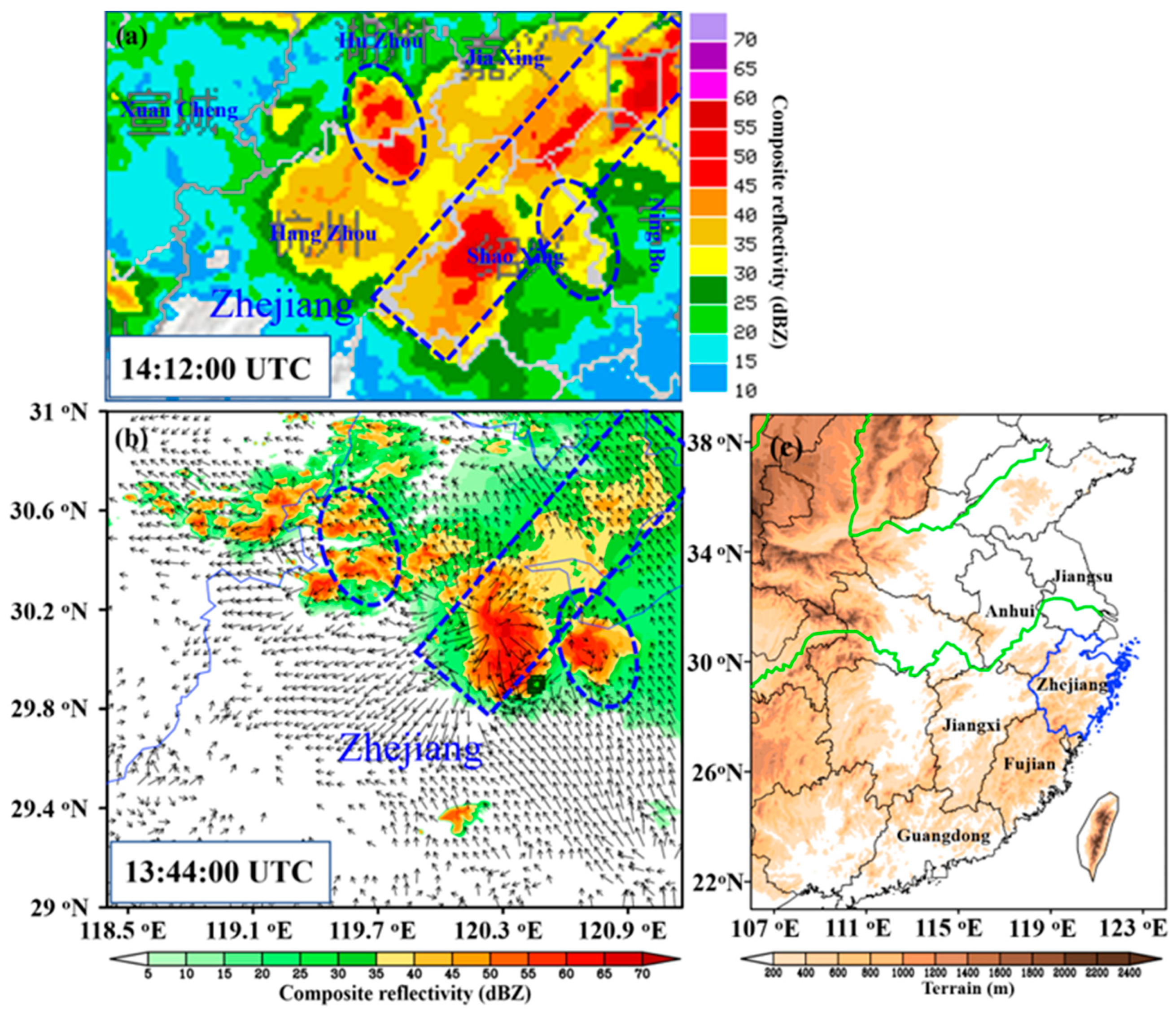
5.1. Horizontal Structure

From 13:24:00 UTC to 13:44:00 UTC 14 May 2021, the southern section of the southwest–northeast-orientated strong reflectivity band (discussed in Section 4) was retained strong intensity (maximum composite radar reflectivity was above 70 dBZ; Figure 6e), as it was associated with a strong small-scale vortex in the lower troposphere (Figure 9c,d). The small-scale vortex was situated within a strong southwesterly low-level jet (Figure 9a,b), which transported abundant moisture and heat into Zhejiang (this was favorable for severe convections). At surface, the strong reflectivity band was mainly associated with a southwest–northeast-orientated high-pressure band (Figure 10), which showed a close relationship to the strong divergent wind at the surface. Affected by the cyclonic wind field associated with the small-scale vortex in the lower troposphere, the southern section of the southwest–northeast-orientated strong reflectivity band rotated counter-clockwise (Figure 6e,f); steered by the middle-level westerly wind (Figure 3b), the strong reflectivity band moved eastward and affected the location where the transmission line towers’ toppling down accident appeared (Figure 6f). Strong surface wind (>17.2 m/s) appeared beneath the strong radar reflectivity band (Figure 7c,d), which caused an intense divergence (Figure 8c,d). Overall, of the surface wind associated with the strong radar reflectivity band, the northerly wind and northwesterly winds were much stronger than the southerly wind and easterly wind. Thus, the former acted as the direct factor for causing the transmission line towers toppling down accident.

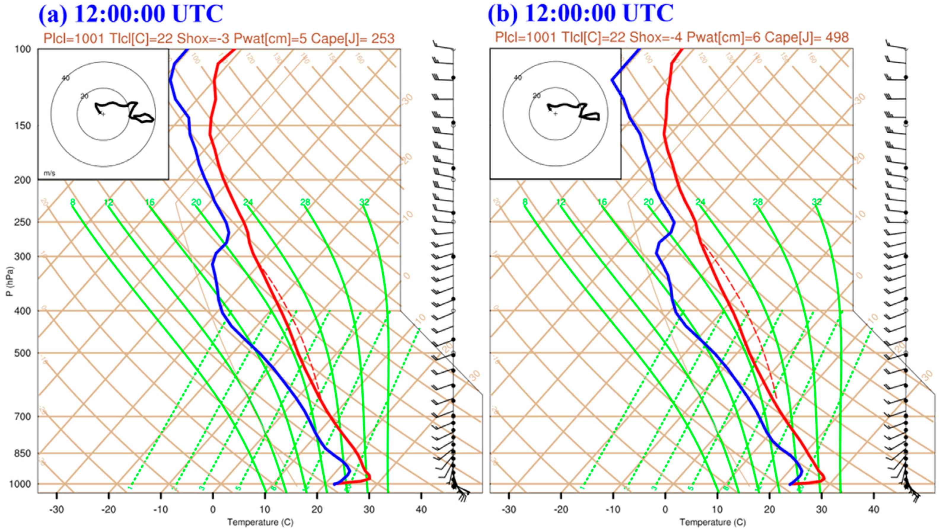
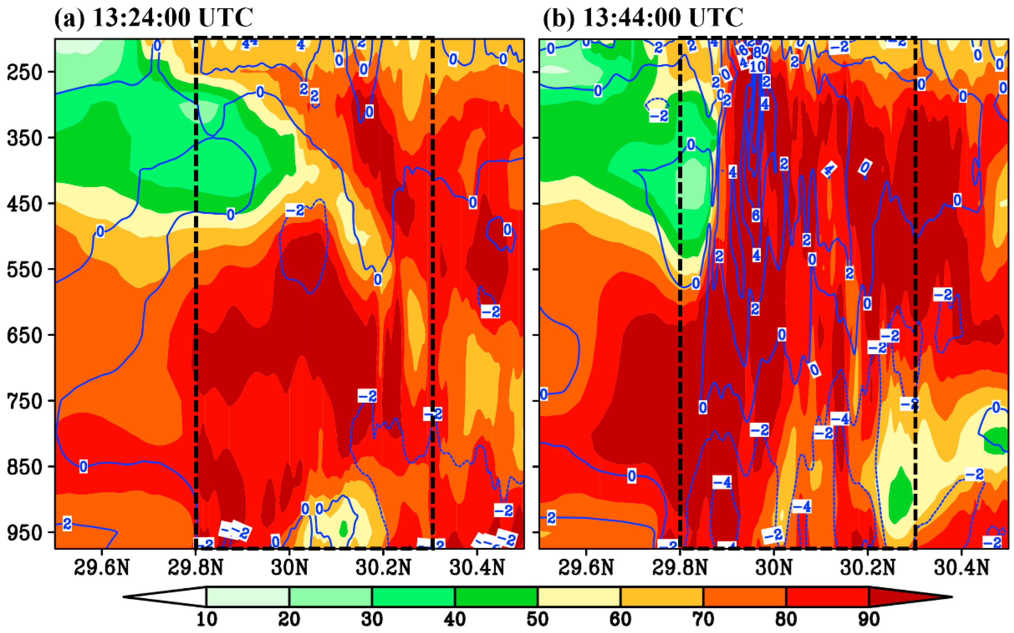
5.2. Vertical Structure

As the southwest–northeast-orientated strong reflectivity band moved eastward and entered the key region (Figure 6d–f), positive geopotential height deviations (the maximum value was above 30 gpm) dominated the near surface layer, particularly for the northern section of the key region (Figure 11). This corresponded to the strong high-pressure zone at the surface (Figure 10b). Below 850 hPa, negative temperature deviations were dominant (Figure 12). This was mainly due to the evaporative cooling of precipitation within the key region (Figure 5b). As Figure 13 shows, strong surface wind centers (≥17.2 m s−1) also appeared in the layer below 850 hPa, which was directly related to the strong winds of the downburst event. Most of these centers were closely associated with the strong descending motions that originated from the middle troposphere, which was a key feature for a downburst event [9,13]. In addition to the strong surface wind centers, strong wind centers (≥30 m s−1) also appeared in the upper troposphere, which were mainly associated with the upper-level jet. The upper-level jet may exert important effects on the lower-level wind speed through downward momentum transport [37,41,48]. Within the key region, the upper tropospheric wind centers did not directly affect the surface wind centers, as there was no downward momentum transport that directly linked them (because there were no obvious downward transport of KE).
Within the key region, the zone with a radar reflectivity zone above 35 dBZ stretched from surface to 200 hPa (Figure 11b), implying the convections were deep. Descending motions mainly appeared in the middle and lower troposphere of the northern section of the key region (Figure 13b), whereas the remainder of the key region was mainly dominated by ascending motions. Above the positive geopotential height deviations in the near surface layer (which were mainly due to evaporative cooling and strong descending motions), there was a thick layer of negative geopotential height deviations (Figure 11b; the minimum value was below −40 gpm). This indicates that at the levels above the near surface layer, the strong convection was mainly associated with low-pressure systems (e.g., the lower tropospheric small-scale vortex, the middle-tropospheric shortwave trough, etc.). In the layer above 850 hPa, there were notable positive temperature deviations (the maximum value was above 4 °C), which were mainly due to the intense condensation-related latent heating. In this layer, the atmosphere is nearly saturated, as the relative humidity was mainly above 90% (Figure 12b). This acted as a crucial condition for the maintenance of the severe convections, since latent heating could promote ascending motions significantly [43,45].

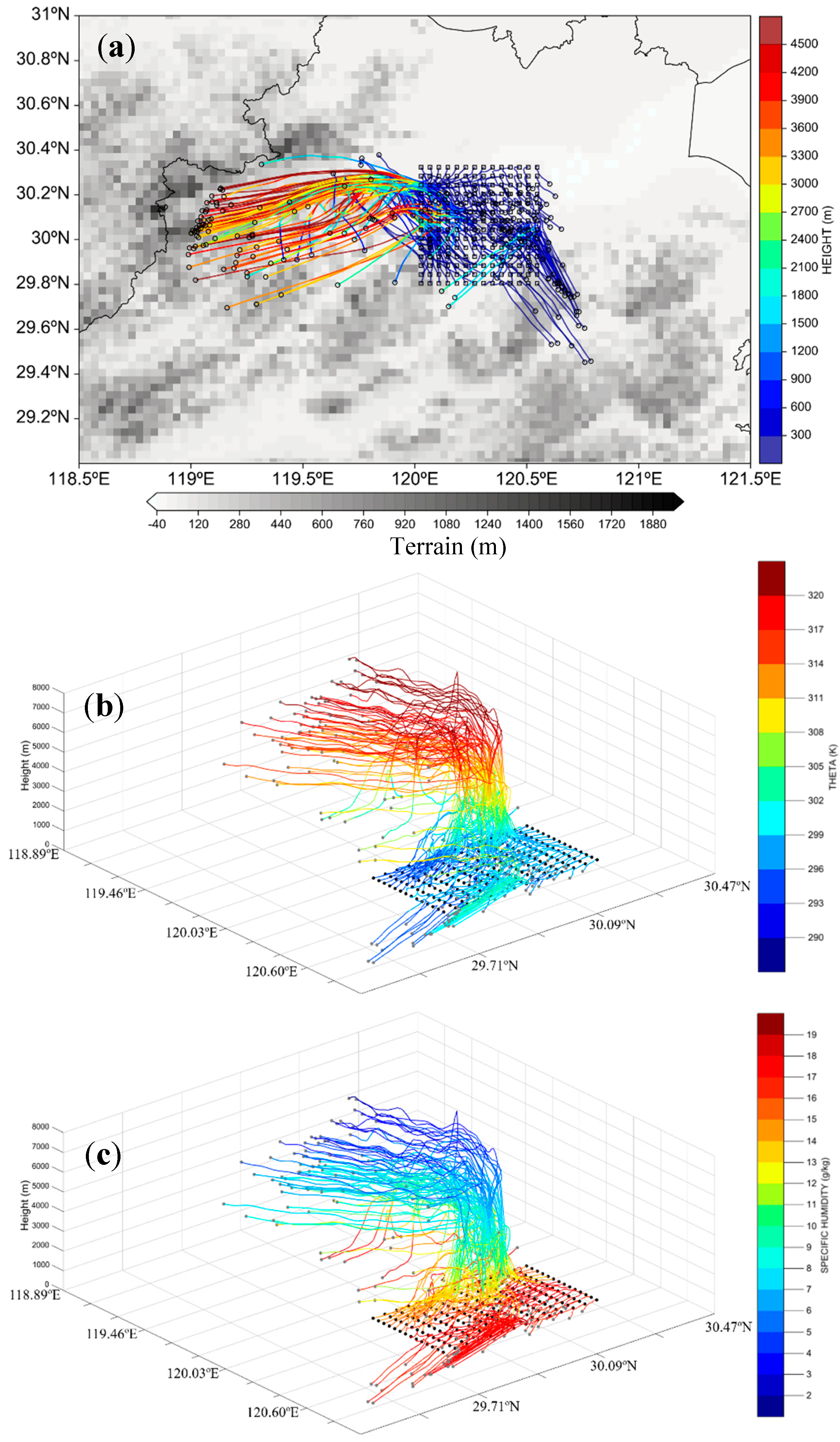
5.3. Backward Trajectory Analysis

In order to analyze the origin of the air particles associated with the strong winds of the downburst event, we used the HYSPLIT model [49] for backward trajectory analyses in this study. The HYSPLIT model is a complete system for computing simple air parcel trajectories, as well as complex transport, dispersion, chemical transformation, and deposition simulations. As the small open circles in Figure 7d show, a total of 196 points (that were evenly distributed with an interval of ~4 km) were used for the backward tracking. All these points were located within the key region of the downburst event, at the height of 10 m (surface wind was observed at this height). We first transferred the 5 min WRF output into the input files for the HYSPLIT model, and then initiated the backward tracking at 13:44:00 UTC 14 May 2021 (when the transmission line towers toppling down accident occurred). The model was run for 2 h to cover the key stage of the downburst event.
As Figure 14a shows, the air particles within the key region mainly came from three areas: (i) the area west of the key region (~61.2% in proportion), (ii) the key region (~18.4%), and (iii) the area southeast of the key region (~20.4%). Overall, the air particles of (i) experienced notable descending processes when they entered the key region (the initial altitude of these air particles were mainly located in the middle troposphere), whereas the air particles of (ii) and (iii) were mainly located in the lower troposphere. Compared with the wind speed of the air particles of (i)–(iii), it was found that most of the air particles of (i) had a surface wind speed above 10 m s−1 (~23.0% of these air particles had a wind speed of above 17.2 m s−1). In contrast, the air particles of (ii) and (iii) mainly showed a surface wind speed below 10 m s−1. Therefore, as mentioned above, the air particles of (i) directly accounted for the strong winds of the downburst event.
From Figure 14b, most of the air particles of (i) had a potential temperature of above 310 K before their descent. Meanwhile, the specific humidity of these air particles was mainly below 9 g kg−1 (Figure 14c), implying that the air was relatively dry (drier air had a larger density). After the air particles of (i) entered the key region, they descended rapidly, mainly due to their larger density and the precipitation drag. During the descent, most of the air particles decreased notably in their potential temperature (most of them decreased by ~10 K; Figure 14b), while they increased significantly in their specific humidity (most of them increased by ~4 g kg−1; Figure 14c). This indicates that intense evaporative cooling occurred during the rapid descending process of the air particles of (i). This rapid cooling produced a strong negative buoyancy [42], which accelerated the descending motions from the middle troposphere to the surface. When the rapid descending air particles reached the surface, they formed a shallow cold high-pressure center and strong divergent winds.

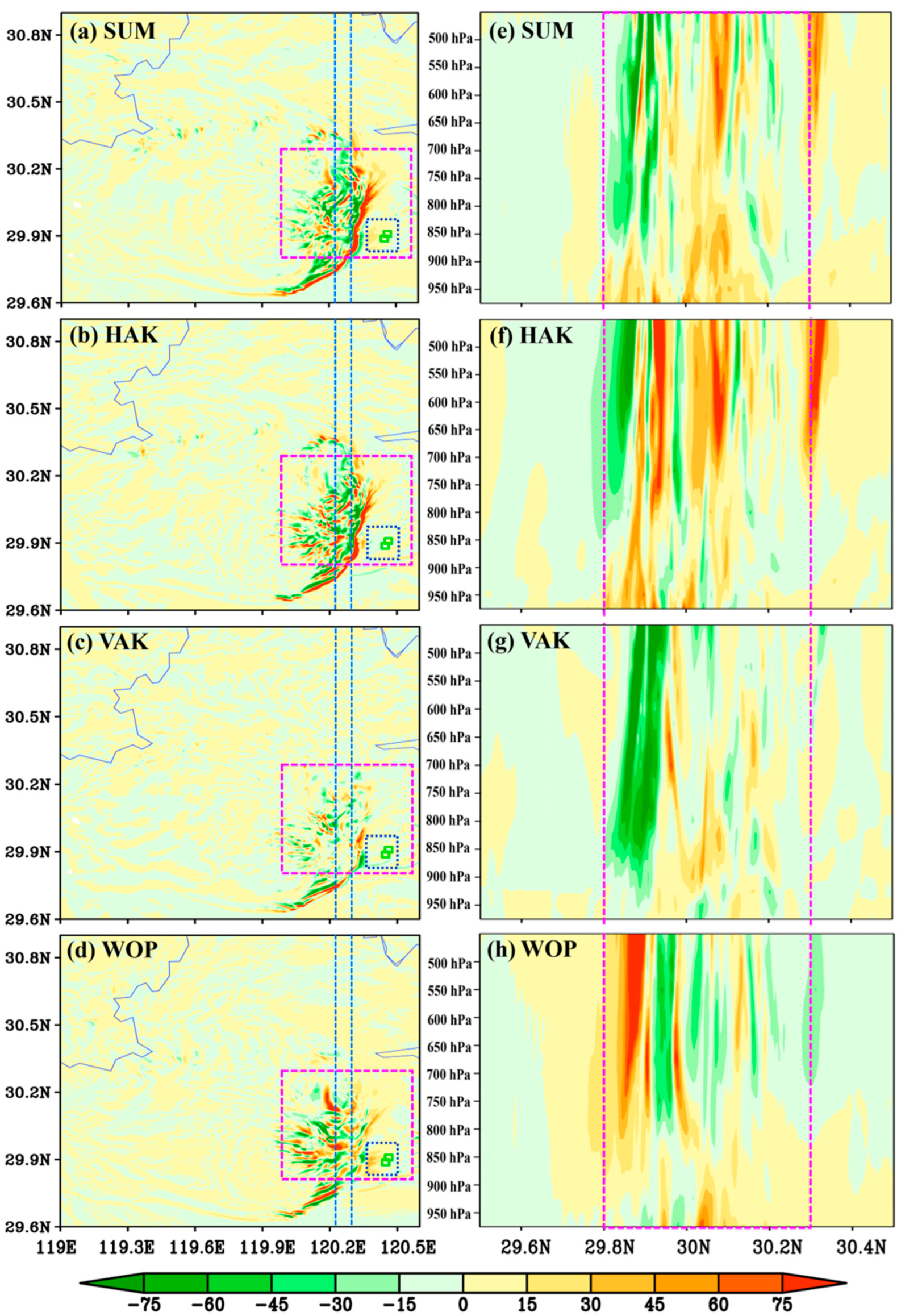
5.4. Kinetic Energy Budget Analyses

Comparison between Figure 7d and Figure 15a shows that, within the key region, the area with a strong positive SUM term was well consistent with the area with a strong surface wind (correlation coefficient was ~0.76). This indicates that the KE budget could effectively reflect the mechanisms that governed the variation in the strong surface wind. For the region surrounding the location where the tower toppling appeared (the small blue dashed box in Figure 15a), it can be found that a strong positive SUM was dominant. This means that the KE increased rapidly within this region, which directly favored the formation of the strong winds that caused the transmission line towers toppling down accident. Comparing Figure 15b–d, it is shown that the term WOP was much stronger than terms HAK and VAK, and thus it was the dominant factor that caused the wind enhancement within this region. As Figure 10b shows, the strong pressure gradient force between the high-pressure closed center (corresponding to intense descending motions) and the low-pressure closed center (corresponding to strong latent heat release) was crucial to cause the strong WOP. In addition to the term WOP, the downward transport of KE (i.e., VAK; Figure 15c) was also conducive to the wind enhancement within the region surrounding the location where the tower toppling appeared, whereas the horizontal transport (i.e., HAK; Figure 15b) mainly resulted in a net export of KE from the region, which decelerated the wind intensification.
Along the strong wind band of the downburst event, there was a strong positive SUM term in the lower troposphere (Figure 15e), implying that the lower-level wind was enhanced. Comparing all the KE budget terms with each other (Figure 15f–h), it could be found that the dominant factors governing the wind enhancement in the northern and southern sections of the key region were notably different. For the northern section, the southward/southeastward-pointing pressure gradient force associated with the strong high-pressure closed center (Figure 10b) did positive work on the strong northwesterly/southerly wind (Figure 7d). This resulted in a strong positive SUM (Figure 15e) which dominated the wind enhancement within the northern section of the key region. For the southern section, the horizontal transport (i.e., HAK; Figure 15f), which resulted in a net import of KE, governed the wind enhancement within this area. Overall, for the whole key region, the vertical transport of KE exerted a nearly neutral effect on the lower-level KE variation along the strong wind band of the downburst event (Figure 15g). This confirmed that the downward transport of the horizontal momentum was not a dominant factor for the formation of the strong surface winds associated with the downburst event.

6. Conclusions and Discussion

On 14 May 2021, six 500 kV transmission line towers in Zhejiang affected by the strong winds associated with a downburst toppled down, resulting in a large range of power outages. Based on the ERA5 reanalysis, we simulated the event by using the mesoscale numerical model WRFv4.4. After confirming that the simulation had reproduced the key features of the background environment and mesoscale systems during the downburst event, we conducted detailed analyses on the evolutionary mechanisms and the 3D structure of the strong winds associated with the downburst event. The main findings are as follows: (i) the downburst event occurred in a favorable background environment, which was characterized by an intense upper-level jet (maintaining an intense upper-level divergence), a strong Western Pacific subtropical high (maintaining a strong northeastward moisture transport), an abundant precipitable water (contributing to intense latent heating), and a strong near-surface vertical wind shear (favoring the maintenance of the severe convection). (ii) A southwest–northeast-orientated, eastward moving (steered by strong middle-level westerly wind) squall line was the parent convection system for the downburst event. The strong surface winds ≥17.2 m s−1 associated with the downburst event, which resulted in an intense divergence, mainly appeared beneath the southern section of the squall line. (iii) The downburst-associated convection was deep, as the convection stretched from the surface to 200 hPa or above. In the near surface layer, the severe convection was mainly associated with a positive geopotential height and negative temperature deviations (mainly due to evaporative cooling and strong descending motions), whereas at the levels above the near surface layer, it was mainly associated with a negative geopotential height and positive temperature deviations (mainly due to intense condensation-related latent heating). (iv) Backward trajectory analysis indicates that the air particles which came from the middle troposphere west of the key region (~61.2% in proportion) were crucial for producing the strong winds of the downburst event. These air particles experienced notable descending processes (mainly due to their larger density and the precipitation drag), during which most of the air particles decreased notably in their potential temperature, while they increased significantly in their specific humidity. This corresponded to intense evaporative cooling, which produced a strong negative buoyancy. This accelerated the descending motions from the middle troposphere to the surface. As the rapid descending air particles reached the surface, they formed a shallow cold high-pressure center and strong divergent winds. (v) Kinetic energy budget analyses denote that, for the region surrounding the location where the tower toppling appeared, the work done by the strong pressure gradient force between the high-pressure closed center (corresponding to intense descending motions) and the low-pressure closed center (corresponding to strong latent heat release) dominated the rapid wind enhancement. In contrast, along the strong wind band of the downburst event, the factors which dominated the wind enhancement in the northern and southern sections of the key region were notably different. For the northern section, the work done by the southward/southeastward-pointing pressure gradient force associated with the strong high-pressure closed center was dominant; for the southern section, the horizontal transport which resulted in a net import of KE into the region governed the wind enhancement. Overall, the downward transport of the horizontal momentum was not a dominant factor for the formation of the strong surface winds associated with the downburst event.
It should be noted that to explore the 3D structure and the evolutionary mechanisms of the downburst events are of great importance to improve the forecast accuracy of this type of event. Although the simulation of this study had reproduced the key features of the downburst event, the maximum surface wind speed was still notably underestimated. How to further improve the forecast accuracy of the strong surface wind? Which factors are decisive to improve the forecast accuracy of a downburst event? We will conduct further researches in the future to address these scientific questions.

Author Contributions

Conceptualization, D.L., J.L. and B.L.; methodology, W.F., D.Y. and X.X.; software, D.L., D.Y. and X.X.; validation, J.L., B.L. and X.X..; formal analysis, D.L., J.L. and B.L.; investigation, D.L., W.F., D.Y. and X.X.; resources, J.L.; data curation, D.L. and X.X.; writing—original draft preparation, D.L., J.L. and B.L.; writing—review and editing, D.L., J.L. and B.L.; visualization, W.F., D.Y. and X.X.; supervision, B.L.; project administration, J.L.; funding acquisition, J.L. All authors have read and agreed to the published version of the manuscript.

Funding

This work was supported by the Science and Technology Foundation of State Grid Corporation of China (grant No. 5200-202219096A-1-1-ZN).

Institutional Review Board Statement

Not applicable.

Informed Consent Statement

Not applicable.

Data Availability Statement

The ECMWF ERA5 reanalysis data can be download at https://www.ecmwf.int/en/forecasts/datasets/reanalysis-datasets/era5 (accessed on 5 September 2022). The GPM IMERG Final Precipitation data can be download at https://gpm.nasa.gov/data/directory (accessed on 5 September 2022).

Acknowledgments

The author would like to thank the ECMWF and NASA for providing the ERA5 reanalysis data (https://www.ecmwf.int/en/forecasts/datasets/reanalysis-datasets/era5; accessed on 5 September 2022) and the GPM IMERG Final Precipitation data (https://gpm.nasa.gov/data/directory; accessed on 5 September 2022). This work was supported by the Science and Technology Foundation of State Grid Corporation of China (grant No. 5200-202219096A-1-1-ZN).

Conflicts of Interest

The authors declare no conflict of interest.

References

  1. Zheng, Y.-G.; Tian, F.-Y.; Meng, Z.-Y.; Xue, M.; Yao, D.; Bai, L.; Zhou, X.; Mao, X.; Wang, M. Survey and Multi-Scale Characteristics of Wind Damage Caused by Convective Storms in the Surrounding Area of the Capsizing Accident of Cruise Ship “Dongfangzhixing”. Meteorol. Mon. 2016, 42, 1–13. [Google Scholar]
  2. American Meteorological Society. 2023. Available online: https://glossary.ametsoc.org/wiki/Downburst (accessed on 5 September 2022).
  3. Fujita, T.T. The Downburst: Microburst and Macroburst, Report of Projects NIMROD and JAWS; Satellite and Mesometeorology Research Project, Department of the Geophysical Sciences, The University of Chicago: Chicago, IL, USA, 1985. [Google Scholar]
  4. PennState. 2023. Available online: https://www.e-education.psu.edu/meteo3/node/2232 (accessed on 5 September 2022).
  5. Meng, Z.; Yao, D.; Bai, L.; Zheng, Y.; Xue, M.; Zhang, X.; Zhao, K.; Tian, F.; Wang, M. Wind estimation around the shipwreck of Oriental Star based on field damage surveys and radar observations. Sci. Bull. 2016, 61, 330–337. [Google Scholar] [CrossRef] [PubMed] [Green Version]
  6. Fujita, T.T. Tornadoes and Downbursts in the Context of Generalized Planetary Scales. J. Atmos. Sci. 1981, 38, 1511–1534. [Google Scholar] [CrossRef]
  7. Smith, T.M.; Elmore, K.L.; Dulin, S.A. A Damaging Downburst Prediction and Detection Algorithm for the WSR-88D. Weather Forecast. 2004, 19, 240–250. [Google Scholar] [CrossRef]
  8. Dotzek, N. Derivation of physically motivated wind speed scales. Atmos. Res. 2009, 93, 564–574. [Google Scholar] [CrossRef] [Green Version]
  9. Kuster, C.M.; Heinselman, P.L.; Schuur, T.J. Rapid-Update Radar Observations of Downbursts Occurring within an Intense Multicell Thunderstorm on 14 June 2011. Weather Forecast. 2016, 31, 827–851. [Google Scholar] [CrossRef]
  10. Bolgiani, P.; Fernández-González, S.; Valero, F.; Merino, A.; García-Ortega, E.; Sánchez, J.L.; Martín, M.L. Simulation of Atmospheric Microbursts Using a Numerical Mesoscale Model at High Spatiotemporal Resolution. J. Geophys. Res. Atmos. 2020, 125, e2019JD031791. [Google Scholar] [CrossRef]
  11. Cai, K.-L.; Yu, X.-D.; Li, C.-L.; Huang, X.-X.; Yan, L.-J.; He, Q.-R.; Mai, W.; Chen, Z. Comparative Analysis of Damage Survey of Microburst in Lingui of Guangxi and Tornado in Zhanjiang of Guangdong in 2019. Meteorol. Mon. 2021, 47, 230–241. [Google Scholar]
  12. Xiao, Y.-J.; Wang, J.; Wang, Z.-B.; Leng, L.; Fu, Z.-K. A Downburst Nowcasting Method Based on Observations of S-Band New Generation Weather Radar. Meteorol. Mon. 2021, 47, 919–931. [Google Scholar]
  13. Wang, Y.; Zheng, Y.-Y.; Zhuang, X.-R.; Zhang, J.; Mu, R.; Sun, K.-Y. Statistical analysis of the structural characteris-tics of typical downbursts in Jiangsu province, China. Acta Meteorol. Sin. 2022, 80, 592–603. [Google Scholar] [CrossRef]
  14. Savory, E.; Parke, G.A.; Zeinoddini, M.; Toy, N.; Disney, P. Modelling of tornado and microburst-induced wind loading and failure of a lattice transmission tower. Eng. Struct. 2001, 23, 365–375. [Google Scholar] [CrossRef]
  15. Shehata, A.; El Damatty, A.; Savory, E. Finite element modeling of transmission line under downburst wind loading. Finite Elem. Anal. Des. 2005, 42, 71–89. [Google Scholar] [CrossRef]
  16. Wang, Z.-G.; Liu, L.; Zhou, X.-Y.; Liu, Y.; Ni, H.-Y.; Li, T.; Pan, F.; Li, D. Cause Analysis of a 500 kV Transmission Line Tower Collapse Incurred by Downburst. Zhejiang Electr. Power 2021, 40, 16–22. [Google Scholar]
  17. Lin, W.; Orf, L.; Savory, E.; Novacco, C. Proposed large-scale modelling of the transient features of a downburst outflow. Wind. Struct. 2007, 10, 315–346. [Google Scholar] [CrossRef]
  18. Bech, J.; Gayà, M.; Aran, M.; Figuerola, F.; Amaro, J.; Arús, J. Tornado damage analysis of a forest area using site survey observations, radar data and a simple analytical vortex model. Atmos. Res. 2009, 93, 118–130. [Google Scholar] [CrossRef]
  19. Vermeire, B.C.; Orf, L.; Savory, E. A parametric study of downburst line near-surface outflows. J. Wind Eng. Ind. Aerodyn. 2011, 99, 226–238. [Google Scholar] [CrossRef]
  20. Lu, M.; Ren, Y.; Xiang, L.; Zhang, B.; Wei, J. Simulation of Phase-to-ground Spacer for Anti-galloping of 500 kV Horizontal Arranged Transmission Lines. Gaodianya Jishu/High Volt. Eng. 2017, 43, 2349–2354. [Google Scholar] [CrossRef]
  21. Colquhoun, J.R. A Decision Tree Method of Forecasting Thunderstorms, Severe Thunderstorms and Tornadoes. Weather Forecast. 1987, 2, 337–345. [Google Scholar] [CrossRef]
  22. Liu, H.; Huang, Q.; Chou, Y.; Tian, H.; Zhang, Y.; Wu, X.; Zhang, J.; Wang, M. A Numerical Study of Downbursts Using the BLASIUS Model. J. Appl. Meteorol. Clim. 2022, 61, 1065–1076. [Google Scholar] [CrossRef]
  23. Hersbach, H.; Bell, B.; Berrisford, P.; Hirahara, S.; Horanyi, A.; Muñoz-Sabater, J.; Nicolas, J.; Peubey, C.; Radu, R.; Schepers, D.; et al. The ERA5 global reanalysis. Q. J. R. Meteorol. Soc. 2020, 146, 1999–2049. [Google Scholar] [CrossRef]
  24. Zhang, Y.-C.; Fu, S.-M.; Sun, J.-H.; Fu, R.; Jin, S.-L.; Ji, D.-S. A 14-year statistics-based semi-idealized modeling study on the formation of a type of heavy rain–producing southwest vortex. Atmos. Sci. Lett. 2019, 20, e894. [Google Scholar] [CrossRef] [Green Version]
  25. Han, Y.; Yang, Q.; Liu, N.; Zhang, K.; Qing, C.; Li, X.; Wu, X.; Luo, T. Analysis of wind-speed profiles and optical turbulence above Gaomeigu and the Tibetan Plateau using ERA5 data. Mon. Not. R. Astron. Soc. 2021, 501, 4692–4702. [Google Scholar] [CrossRef]
  26. Huang, L.; Mo, Z.; Liu, L.; Zeng, Z.; Chen, J.; Xiong, S.; He, H. Evaluation of Hourly PWV Products Derived From ERA5 and MERRA-2 Over the Tibetan Plateau Using Ground-Based GNSS Observations by Two Enhanced Models. Earth Space Sci. 2021, 8, e2020EA001516. [Google Scholar] [CrossRef]
  27. Xin, Y.; Liu, J.; Liu, X.; Liu, G.; Cheng, X.; Chen, Y. Reduction of uncertainties in surface heat flux over the Tibetan Plateau from ERA-Interim to ERA5. Int. J. Clim. 2022, 42, 6277–6292. [Google Scholar] [CrossRef]
  28. Huffman, G.J.; Stocker, E.F.; Bolvin, D.T.; Nelkin, E.J.; Tan, J. GPM IMERG Final Precipitation L3 1 Day 0.1 Degree × 0.1 Degree V06; Savtchenko, A., Ed.; Goddard Earth Sciences Data and Information Services Center (GES DISC): Greenbelt, MD, USA, 2019.
  29. Skamarock, W.C.; Klemp, J.B.; Dudhia, J.; Gill, D.O.; Barker, D.M.; Duda, M.G.; Huang, X.-Y.; Wang, W.; Powers, J.G. A Description of the Advanced Research WRF Version 3; NCAR: Boulder, CO, USA, 2008. [Google Scholar] [CrossRef]
  30. Di Bernardino, A.; Mazzarella, V.; Pecci, M.; Casasanta, G.; Cacciani, M.; Ferretti, R. Interaction of the Sea Breeze with the Urban Area of Rome: WRF Mesoscale and WRF Large-Eddy Simulations Compared to Ground-Based Observations. Bound.-Layer Meteorol. 2022, 185, 333–363. [Google Scholar] [CrossRef]
  31. Chen, F.; Dudhia, J. Coupling an Advanced Land Surface–Hydrology Model with the Penn State–NCAR MM5 Modeling System. Part I: Model Implementation and Sensitivity. Mon. Weather Rev. 2001, 129, 569–585. [Google Scholar] [CrossRef]
  32. Hong, S.-Y.; Noh, Y.; Dudhia, J. A New Vertical Diffusion Package with an Explicit Treatment of Entrainment Processes. Mon. Weather Rev. 2006, 134, 2318–2341. [Google Scholar] [CrossRef] [Green Version]
  33. Hong, S.-Y.; Lim, J. The WRF Single-Moment 6-Class Microphysics Scheme (WSM6). Asia-Pac. J. Atmos. Sci. 2006, 42, 129–151. [Google Scholar]
  34. Dudhia, J. Numerical Study of Convection Observed during the Winter Monsoon Experiment Using a Mesoscale Two-Dimensional Model. J. Atmos. Sci. 1989, 46, 3077–3107. [Google Scholar] [CrossRef]
  35. Mlawer, E.J.; Taubman, S.J.; Brown, P.D.; Iacono, M.J.; Clough, S.A. Radiative transfer for inhomogeneous atmospheres: RRTM, a validated correlated-k model for the longwave. J. Geophys. Res. Atmos. 1997, 102, 16663–16682. [Google Scholar] [CrossRef] [Green Version]
  36. Ma, H.; Cao, X.; Ma, X.; Su, H.; Jing, Y.; Zhu, K. Improving the Wind Power Density Forecast in the Middle- and High-Latitude Regions of China by Selecting the Relatively Optimal Planetary Boundary Layer Schemes. Atmosphere 2022, 13, 2034. [Google Scholar] [CrossRef]
  37. Shikhovtsev, A.Y.; Kovadlo, P.G.; Lezhenin, A.A.; Korobov, O.A.; Kiselev, A.V.; Russkikh, I.V.; Kolobov, D.Y.; Shikhovtsev, M.Y. Influence of Atmospheric Flow Structure on Optical Turbulence Characteristics. Appl. Sci. 2023, 13, 1282. [Google Scholar] [CrossRef]
  38. Fu, S.; Yu, F.; Wang, D.; Xia, R. A comparison of two kinds of eastward-moving mesoscale vortices during the mei-yu period of 2010. Sci. China Earth Sci. 2013, 56, 282–300. [Google Scholar] [CrossRef]
  39. Fu, S.-M.; Liu, R.-X.; Sun, J.-H. On the Scale Interactions that Dominate the Maintenance of a Persistent Heavy Rainfall Event: A Piecewise Energy Analysis. J. Atmos. Sci. 2018, 75, 907–925. [Google Scholar] [CrossRef]
  40. Li, W.; Xia, R.; Sun, J.; Fu, S.; Jiang, L.; Chen, B.; Tian, F. Layer-Wise Formation Mechanisms of an Entire-Troposphere-Thick Extratropical Cyclone That Induces a Record-Breaking Catastrophic Rainstorm in Beijing. J. Geophys. Res. Atmos. 2019, 124, 10567–10591. [Google Scholar] [CrossRef]
  41. Fu, S.; Jin, S.; Shen, W.; Li, D.; Liu, B.; Sun, J. A kinetic energy budget on the severe wind production that causes a serious state grid failure in Southern Xinjiang China. Atmos. Sci. Lett. 2020, 21, e977. [Google Scholar] [CrossRef]
  42. Holton, J.R. An Introduction to Dynamic Meteorology, 4th ed.; Elsevier Academic Press: Burlington, MA, USA, 2004. [Google Scholar]
  43. Fu, S.-M.; Mai, Z.; Sun, J.-H.; Li, W.-L.; Ding, Y.; Wang, Y.-Q. Impacts of Convective Activity over the Tibetan Plateau on Plateau Vortex, Southwest Vortex, and Downstream Precipitation. J. Atmos. Sci. 2019, 76, 3803–3830. [Google Scholar] [CrossRef]
  44. Fu, S.; Zhang, Y.; Wang, H.; Tang, H.; Li, W.; Sun, J. On the Evolution of a Long-Lived Mesoscale Convective Vortex that Acted as a Crucial Condition for the Extremely Strong Hourly Precipitation in Zhengzhou. J. Geophys. Res. Atmos. 2022, 127, e2021JD036233. [Google Scholar] [CrossRef]
  45. Fu, S.; Mai, Z.; Sun, J.; Li, W.; Zhong, Q.; Sun, J.; Zhang, Y. A semi-idealized modeling study on the long-lived eastward propagating mesoscale convective system over the Tibetan Plateau. Sci. China Earth Sci. 2021, 64, 1996–2014. [Google Scholar] [CrossRef]
  46. Fu, S.-M.; Sun, J.-H.; Luo, Y.-L.; Zhang, Y.-C. Formation of Long-Lived Summertime Mesoscale Vortices over Central East China:Semi-Idealized Simulations Based on a 14-Year Vortex Statistic. J. Atmos. Sci. 2017, 74, 3955–3979. [Google Scholar] [CrossRef]
  47. Etherton, B.; Santos, P. Sensitivity of WRF Forecasts for South Florida to Initial Conditions. Weather Forecast. 2008, 23, 725–740. [Google Scholar] [CrossRef] [Green Version]
  48. Hach, Y.; Jabiri, A.; Ziad, A.; Bounhir, A.; Sabil, M.; Abahamid, A.; Benkhaldoun, Z. Meteorological profiles and op-tical turbulence in the free atmosphere with NCEP/NCAR data at Oukaïmeden—I. Meteorological parameters analysis and tropospheric wind regimes. Mon. Not. R. Astron. Soc. 2011, 420, 637–650. [Google Scholar] [CrossRef] [Green Version]
  49. Stein, A.F.; Draxler, R.R.; Rolph, G.D.; Stunder, B.J.B.; Cohen, M.D.; Ngan, F. NOAA’s HYSPLIT Atmospheric Transport and Dispersion Modeling System. Bull. Am. Meteorol. Soc. 2015, 96, 2059–2077. [Google Scholar] [CrossRef]
Figure 1. (a) Observed composite radar reflectivity (shading; dBZ) at 14:12:00 UTC 14 May 2021, where the dashed rectangle and ellipses mark the sections used for comparisons. (b) Simulated composite radar reflectivity (shading; dBZ), and surface wind (vector) at 13:44:00 UTC 14 May 2021, where the small green boxes mark the locations at which the tower toppling appeared, and the dashed rectangle and ellipses mark the sections used for comparisons. (c) Terrain (shading; m) and distribution of provinces, where the blue map highlights Zhejiang Province.
Atmosphere 14 00427 g001
Figure 2. Three domains (d01–d03) for the simulations in this study, where the numbers in the parentheses show the total grids and grid spacing for each domain.
Atmosphere 14 00427 g002
Figure 3. Panel (a) shows that 200 hPa wind (shading and wind barb; m s−1), 500 hPa geopotential height (black contour; gpm) and 500 hPa temperature (red contour; °C) derived from ERA5 reanalysis, where the thick dashed line is the trough line and the small green boxes mark the location at which the tower toppling appeared. Panel (b) is the same as (a) but for the simulation.
Atmosphere 14 00427 g003
Figure 4. Panel (a) is the simulated hodograph and skew-T plot of 12:00:00 UTC 14 May 2021 at the location where transmission line towers toppling appeared. Panel (b) is the same as (a) but for the ERA5-based hodograph and skew-T plot. Plcl = pressure of the lifted condensation level (hPa); Tlcl = temperature of the lifted condensation level (°C); shox = showalter index; Pwat = precipitable water (cm); Cape = convective availabe potenrial energy (J kg−1).
Atmosphere 14 00427 g004
Figure 5. Panel (a) shows the observed (GPM) 3 h accumulated precipitation from 12:00:00 UTC to 15:00:00 UTC, 14 May 2021 (shading; mm), where the small black boxes mark the locations at which the tower toppling appeared. Panel (b) is the same as (a) but for the simulation.
Atmosphere 14 00427 g005
Figure 6. Panels (af) show the simulated composite radar reflectivity (shading; dBZ) and surface wind speed ≥3 m s−1 (vectors; m s−1), where the blue ellipses outline the targeted system, and the purple dashed boxes show the key region.
Atmosphere 14 00427 g006
Figure 7. Panels (ad) show the simulated surface wind speed (shading; m s−1) and vector (arrows; m s−1) at typical stages of the event. The dashed purple box marks the regions where the downburst appeared, the small blue open circles show the locations for backward tracking, the small green boxes mark the locations at which the tower toppling appeared, and the two dashed lines mark the band (from 120.24° E to 120.32° E) for calculating the averaged cross section.
Atmosphere 14 00427 g007
Figure 8. Panels (ad) show the simulated surface wind vector (arrows; m s−1) and its divergence (shading; 10−3 s−1) at typical stages of the event. The dashed purple box marks the regions where the downburst appeared, the small blue open circles show the locations for backward tracking, the small green boxes mark the locations at which the tower toppling appeared, and the two dashed lines mark the band (from 120.24° E to 120.32° E) for calculating the averaged cross section.
Atmosphere 14 00427 g008
Figure 9. Panels (a,b) show the geopotential height (black contour; gpm), temperature (red contour; °C), wind speed (shading; m s−1), and wind above 8 m s−1 (a full bar is 10 m s−1) at 850 hPa, where the small green boxes mark the locations at which the tower toppling appeared and the small blue box shows the key region. Panels (c,d) show the 850 hPa stream field, vorticity (shading; 10−3 s−1) and wind above 10 m s−1 (a full bar is 10 m s−1), where the small green boxes mark the locations at which the tower toppling appeared and the green dashed boxes show the key region.
Atmosphere 14 00427 g009
Figure 10. Panels (a,b) show the horizontal wind speed (shading; m s−1) and sea level pressure (black contour; hPa) at typical stages, where the purple boxes mark the key region, and the small green boxes mark the locations at which the tower toppling appeared. H = high pressure center; L = low pressure center.
Atmosphere 14 00427 g010
Figure 11. Panels (a,b) show the averaged (from 120.24° E to 120.32° E) cross section of the horizontal radar reflectivity (shading; dBZ) and geopotential height deviation (blue contour; gpm) at typical stages, where the black dashed lines mark the key region. The ordinate is pressure and the abscissa is latitude.
Atmosphere 14 00427 g011
Figure 12. Panels (a,b) show the averaged (from 120.24° E to 120.32° E) cross section of the relative humidity (shading; %) and temperature deviation (blue contour; °C) at typical stages, where the black dashed lines mark the key region. The ordinate is pressure and the abscissa is latitude.
Atmosphere 14 00427 g012
Figure 13. Panels (a,b) show the averaged (from 120.24° E to 120.32° E) cross section of the horizontal wind speed (shading; m s−1) and descending motions (blue contour; m s−1) at typical stages, where the black dashed lines mark the key region. The ordinate is pressure and the abscissa is latitude.
Atmosphere 14 00427 g013
Figure 14. Panel (a) illustrates the trajectories of 196 points (small blue boxes) within the key region, where the shading is their height (m), small black circles show their starting locations, and the gray shading are the terrain (m). Panel (b) is the 3D illustration of the trajectories of 196 points (small black dots) within the key region, where the shading is their potential temperature (K) and gray points are their starting locations. Panel (c) is the same as (b) but for the specific humidity (g kg−1).
Atmosphere 14 00427 g014
Figure 15. Panels (ad) show the KE budget terms (shading; 10−2 W kg−1) at 13:44:00 UTC 14 May 2021 (at the height of 500 m), where the purple dashed boxes show the key regions, the small green boxes mark the locations at which the tower toppling appeared, the blue dashed boxes show the region surrounding the tower toppling locations, and the two dashed blue lines mark the band (from 120.24° E to 120.32° E) for calculating the averaged cross section. Panels (eh) show the averaged (from 120.24° E to 120.32° E) cross section of the KE budget terms (shading; 10−2 W kg−1) at 13:44:00 UTC 14 May 2021, where the purple dashed lines mark the key region.
Atmosphere 14 00427 g015
Disclaimer/Publisher’s Note: The statements, opinions and data contained in all publications are solely those of the individual author(s) and contributor(s) and not of MDPI and/or the editor(s). MDPI and/or the editor(s) disclaim responsibility for any injury to people or property resulting from any ideas, methods, instructions or products referred to in the content.

