Medium- and Long-Term Wind-Power Forecasts, Considering Regional Similarities

Abstract

Accurate and efficient medium- and long-term forecasts of wind power can provide technical support for the efficient development and utilization of wind resources. Considering the regional characteristics of wind resources, the regional-similarity factor was introduced into the study of wind-power forecasting, and, to assess the long-term dependence of wind power, the long-short-term-memory method was selected for medium- and long-term forecasting of wind-power trends in a case study carried out in Northwest China. The results showed that the forecasting error of the presented method was reduced by an average of 20.80%, compared with the forecasting of individual stations, which verified the effectiveness of considering the regional characteristics in wind-resource prediction. Different area-division methods resulted in different effects on prediction accuracy. This study provides a new approach and a reference for medium- and long-term wind-resource prediction.

1. Introduction

Wind resources are one of the new energy sources with broad development prospects, and large-scale promotion of wind power could make a positive contribution to the “dual carbon goals” [1]. Highly accurate medium- and long-term forecasts of wind power can effectively reduce the rate of abandoned wind, and play an important role in the efficient exploitation of wind resources. Wind resources show regional characteristics on the medium- and long-term time scales, particularly in the vast and expansive northwest region. Medium- and long-term wind power forecasting based on regional characteristics could help to improve the forecast accuracy, and thus provide technical support for the development and utilization of wind resources.

In response to the regional characteristics of wind resources [2], many researchers have carried out further studies. Peijun, S et al. [3] used the trend-change value and fluctuation-characteristic value of annual wind speed in China from 1961 to 2012 to quantitatively identify the regional characteristics of wind speed in China. According to the former, the country was divided into six first-level trend zones, and, according to the latter, it was divided into 12 secondary-fluctuation-characteristic areas. For the northwest region, Ding, C.X et al. [4] analyzed the average wind speed of 105 meteorological stations for approximately 50 years, and the results showed that the spatial variation of wind speed in the northwest region shows a trend of increasing in the east and west and decreasing in the central areas. Luo, W et al. [5] studied the regional characteristics of wind speed in Northwest China and pointed out the discontinuous-wind-speed distribution, with obvious extreme-value centers and a tendency for the distribution to be larger in the east and smaller in the west. A large number of studies have noted that wind-energy resources in the northwest have massive storage capacity and distinct regional characteristics.

Medium- and long-term forecasting of wind power refers to the achievement of time scales including annual, seasonal, and monthly forecasts by physical-modeling methods or statistical methods [6]. The physical causal-analysis method establishes physical models by analyzing the effects of obstacles, surface roughness, contour lines, temperature, atmospheric pressure, and other factors around wind farms regarding wind speed [7]. Commonly-used mathematical and statistical methods include the autoregressive–moving-average [8], probabilistic prediction, gray forecast [9], wavelet analysis [10], Markov chain [11], rough set theory [12], and deep learning [13]. In recent years, with the continuous development of deep learning in artificial intelligence, new machine-learning methods have emerged and been widely used in the field of new-energy forecasting, adding new methods and approaches for the medium- and long-term forecasting of wind power.

LSTM is preferred over other algorithms because the LSTM network can study the non-stationary nature of the time series which reduces forecasting errors [14]. Wang, Y et al. [15] constructed a weighted, combined-LSTM (long-short-term-memory)–XGBoost (eXtreme-Gradient-Boosting) prediction model, which had higher prediction accuracy than a single model. Han, S et al. [16] proposed a joint medium- and long-term wind-power and photovoltaic-power-capacity forecasting model based on the copula function and LSTM model. The validity and applicability of the method were confirmed using actual data from wind farms and PV-power plants in China and the United States. Sun, S et al. [6] constructed an adaptive-forecasting model based on the GWO (grey-wolf-optimizer) algorithm and LSTM to achieve the total electricity forecasting of a coastal wind farm and region, and the performance of the forecasting model was found to be superior.

With the gradual growth in the proportion of wind power connected to the grid, the traditional single-station forecasting model has not adapted to the development pattern of centralized large-scale wind-power development in China [17]. The existing medium- and long-term forecasts of wind power are mostly for individual sites, all of which have certain shortcomings, such as ignoring the regional characteristics. Lu, J et al. [18] constructed an ARFIMA (auto-regressive-integrated-moving-average) long-memory time-series model, which improved the accuracy of wind-power forecasting and selected a single site for validation. Shan, B et al. [19] constructed a combined model of the improved beetle-antennae-search algorithm for single-site wind-power forecasting at 2448 sample points of the Sotavento wind farm in Galicia, Spain; however, regional characteristics were not considered. Therefore, there is an urgent need to include regional characteristics in wind-resource forecasting, to improve its accuracy.

In view of this, this paper proposes a method introducing the regional characteristics of wind resources, by selecting LSTM, which is more suitable for medium- and long-term forecasts, and constructing a medium- and long-term-forecast model of wind-power trends based on regional similarities, and taking the northwest region of China as a case study to test the presented method.

2. Research Methods

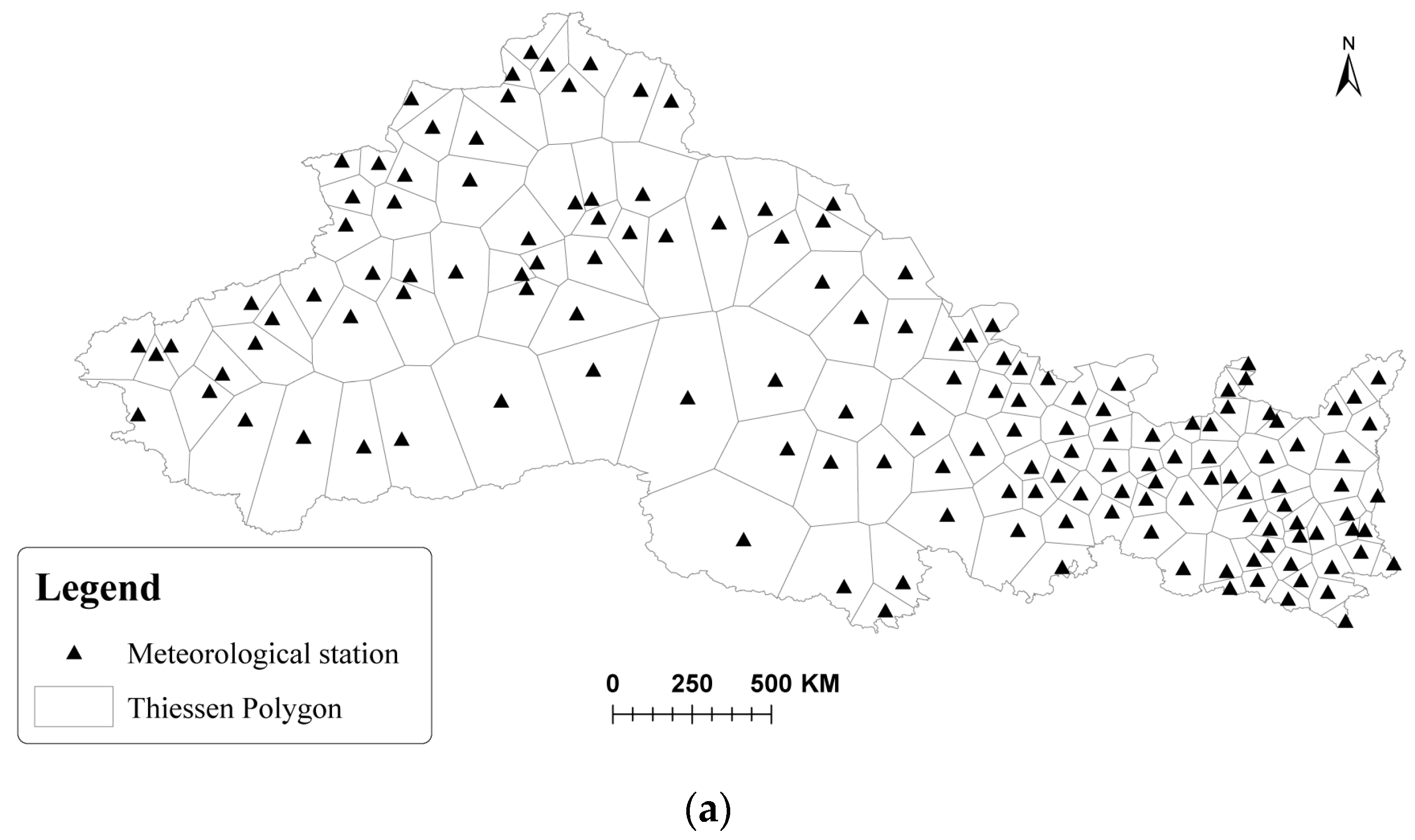
2.1. Data Preprocessing

We selected five provinces, Qinghai, Xinjiang, Gansu, Ningxia, and Shanxi (hereinafter referred to as the five provinces of Northwest China), as the research area. A total of 56 years of monthly average wind-speed series from 1961 to 2016 at 153 wind-speed-observation stations in this area were used as the basic data.

First, the wind speed at a height of 10 m above ground (results of meteorological-station observations) was converted to the wind speed at a height of 80 m above ground (the height of the hub of the wind turbine).

$$v=v_1\times {\left(\frac{h}{h_1}\right)}^{\alpha }$$

(1)

In Equation (1), $v_1$ is the wind speed at the height of $h_1$; $v$ is the wind speed at the target height, $h$; and $\alpha$ is the wind-shear index, with values in the range of [0.125, 0.5]. Studies have shown that the wind-shear index in the five provinces of Northwest China is [0.1, 0.2], apart from two areas in Mangya of Xinjiang and Gangcha of Qinghai, where the wind-shear index is [0, 0.1] [20]. For ease of calculation, the wind-shear index in Mangya and Gangcha counties was recorded as 0.1; in other areas, the wind-shear index was taken as an approximation of 0.143. when the measured wind-speed data at different heights were not available in the “wind energy resource assessment method for wind farms (GB/T 18710-2002)” [21].

Next, the air density in the area where the meteorological station is located was calculated. According to the electric-power-industry standard of the People’s Republic of China, “Technical Regulations for Design and Calculation of Thermal Power Plant Combustion System (DL/T 5240-2010)” [22], issued by the National Energy Administration, the equation between atmospheric pressure and altitude is as follows:

$$P_{\alpha }=0.143\times {\left[1-0.0225\times \frac{H}{1000}\left(\frac{6357}{6357+\frac{H}{1000}}\right)\right]}^{5.256}$$

(2)

In Equation (2), $P_{\alpha }$ is the average atmospheric pressure of the place, kPa, and $H$ is the altitude of the place, m.

The air density in the region was calculated from the atmospheric pressure and temperature, based on the formula as shown in Equation (3):

$$\rho =\frac{P_{\alpha }}{0.2869\times \left(T+273.1\right)}$$

(3)

In Equation (3), $\rho$ is the air density, kg/m³, and $T$ is the temperature, °C.

Finally, the power curve (rated power 3000 kW) of a wind-turbine-generator set of a certain manufacturer was adopted, and the power at the corresponding wind speed and air density was calculated, using a linear-interpolation method.

2.2. Forecast Method

The medium- and long-term wind-power-forecast method based on regional similarities proposed in this paper consists of two parts: the whole study area was divided into several sub-regions, based on regional similarities, and then the LSTM method was used for each sub-region for medium- and long-term-forecasting of wind power. The flowchart of the proposed method is shown in Figure 1.

2.2.1. Wind-Power Trend Fitting

The estimated wind-power data often show various uncertainty phenomena, including fluctuations and peaks, whose nonlinear and non-stationary characteristics will reduce the performance of LSTM prediction [23]. Therefore, when forecasting in this paper, the fractal-adaptive-moving-average (FRAMA) method was first used to obtain the trend of the wind power, and then LSTM was used to forecast the trend of the wind power. Fractal adaptive moving average (FRAMA), proposed by John Ehlers, was created based on the exponential-moving-average algorithm [24], which has the advantage of following the violent trend movement and slowing down significantly when the data are combined [25].

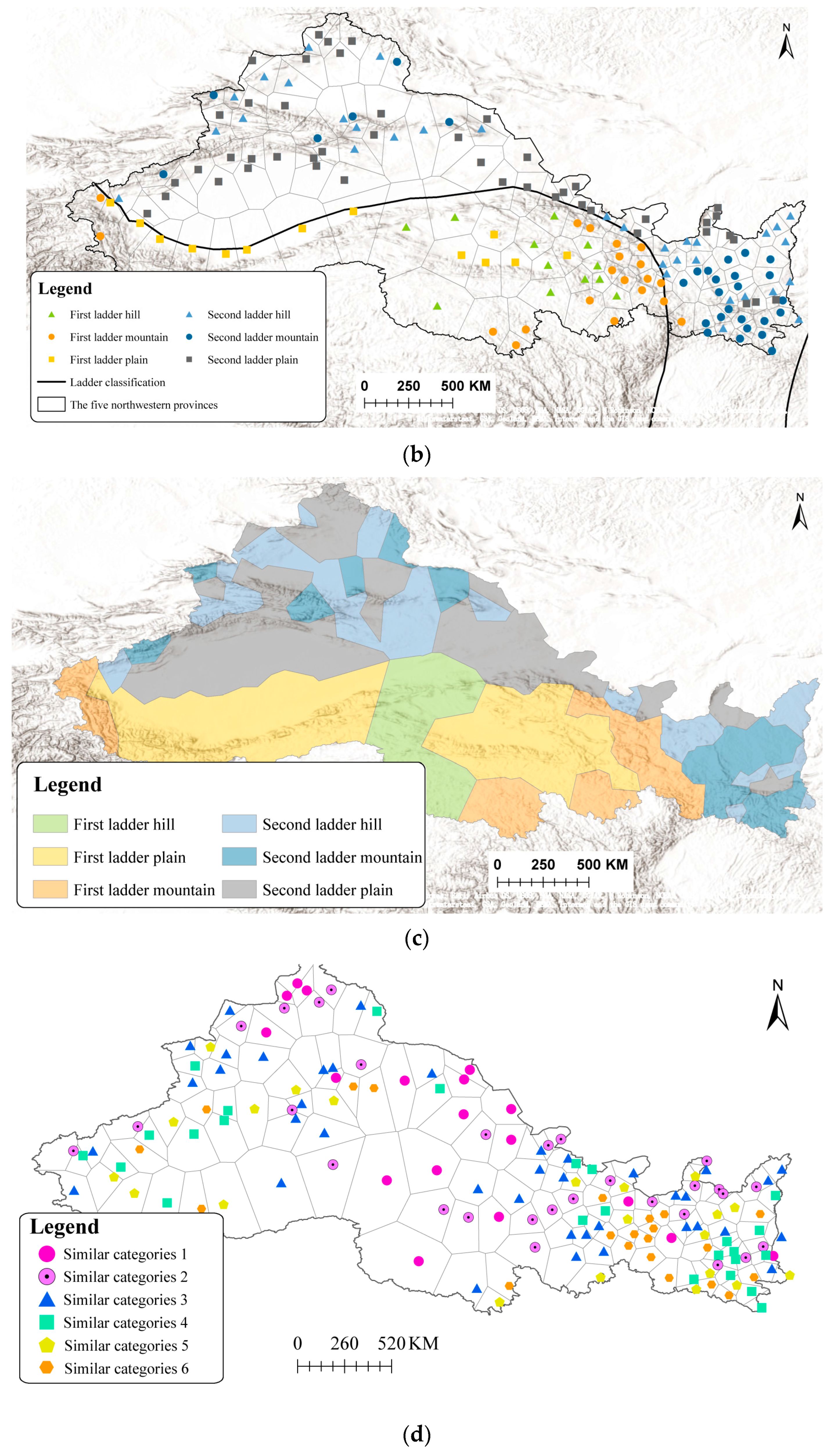
2.2.2. Region-Division Method Based on Regional Similarities

The Thiessen-polygon method was primarily used to divide all the stations in the study area into small areas, and then the similarity between different sites was judged according to the centroid distance of the wind-power time series, and finally, the stations with high similarity and close geographical characteristics (location, altitude, terrain and other conditions) were combined into a sub-region. The steps of the similarity calculation method are given below.

The centroid-similarity calculation method [26] first analyzed the time-series process line as being composed of N point connections, divided the process line into N-1 trapezoidal columns, and then calculated the area and centroid coordinates of each trapezoidal column, obtained the relative position of the centroid coordinates of the process line, and finally calculated the distance between the centroid coordinates of the two process lines as the similarity distance. The specific calculation process is as follows:

• Analysis of the wind-power process line.

The wind-power process line was obtained in a right-angle coordinate system with time, $x$, as the horizontal coordinate and wind power, $y$, as the vertical coordinate. The analysis process included analyzing the wind-power process line as composed of several connected points, assuming that there are a total of $N$ points, which were used as control points and numbered from left to right in order, as $1,2,\dots ,N,N\ge 2$. The coordinates of the kth control point were $\left(x_k,y_k\right),k=1,2,\dots ,N$.

2.

Segmentation of the wind-power process line.

The wind-power process line was divided into $N\text{-}1$ trapezoidal columns, and the four coordinate points $\left(x_i,0\right),\left(x_{i+1},0\right),\left(x_i,y_i\right),\left(x_{i+1},y_{i+1}\right)$ were connected first and last, to form closed trapezoidal columns, $i=1,2,\dots ,N\text{-}1$.

3.

Calculation of the area of trapezoidal column, $i$, and the coordinates of its centroid.

Area of $A_i$, trapezoidal column $i$:

$$A_i=\left(y_i+y_{i+1}\right)\times \left(x_{i+1}+x_i\right)/2$$

(4)

Centroid horizontal coordinate, $x_i^{cen}$, of trapezoidal column, $i$:

$$x_i^{cen}=\left(x_i+x_{i+1}\right)/2$$

(5)

Centroid vertical coordinate $y^{cen}$ of trapezoidal column, $i$:

$$y_i^{cen}=\left(y_i+y_{i+1}\right)/2$$

(6)

4.

Calculation of the line centroid coordinates of the wind-power process.

Wind-power process-line centroid horizontal coordinate, $x^{cen}$:

$$x^{cen}=\frac{{\sum }_{i=1}^{N-1}\left(A_i+x_i^{cen}\right)}{{\sum }_{i=1}^{N-1}{A}_i}$$

(7)

Wind-power process-line centroid vertical coordinate, $y^{cen}$:

$$x^{cen}=\frac{{\sum }_{i=1}^{N-1}\left(A_i+y_i^{cen}\right)}{{\sum }_{i=1}^{N-1}{A}_i}$$

(8)

5.

Process-line centroid relative-position calculation.

Wind-power process-line centroid horizontal relative position $, x_{rel}^{cen}$:

$$x_{rel}^{cen}=\left(x^{cen}-x^{mi{n}^{ma{x}^{min}}}\right)$$

(9)

Wind-power process-line centroid vertical relative position, $y_{rel}^{cen}$:

$$y_{rel}^{cen}=\left(y^{cen}-y^{mi{n}^{ma{x}^{min}}}\right)$$

(10)

According to the above formulas, $x^{max}$ and $x^{min}$ are the maximum and minimum values of time respectively, and $y^{max}$ and $y^{min}$ are the maximum and minimum values of wind-power velocity, respectively.

6.

Calculation of the wind-power process-line similar distance.

After calculating the relative positions of the centroid of the wind-power process lines at each station according to steps 1 to 5, the similarity distance between two wind-power process lines was calculated by the following equation:

$$D_{mn}=\sqrt{\frac{{(x_{rel}^{cen,m}-x_{rel}^{cen,n})}^2+{(y_{rel}^{cen,m}-y_{rel}^{cen,n})}^2}{2}}$$

(11)

In Equation (11), $D_{mn}$ is the similarity distance between the wind-power process line at the $m$th station and the wind-power process line at the $n$th station, $x_{rel}^{cen,m}$ is the horizontal relative position of the centroid of the wind-power process line at the $m$th station, $y_{rel}^{cen,m}$ is the vertical relative position of the centroid of the wind-power process line at the $m$th station, $x_{rel}^{cen,n}$ is the horizontal relative position of the centroid of the wind-power process line at the $n$th station, and $y_{rel}^{cen,n}$ is the vertical relative position of the centroid of the wind-power process line at the $n$th station.

After completing the similar-distance calculation, the stations needed to be classified. According to Equation (11), each station was given a similar distance value to other stations. With a total of 153 wind-speed measuring stations in Northwest China, a 153 × 153 wind-power similarity-distance matrix, $D$, could be obtained; the similarity distance was sorted from small to large in the column direction, and it was noted that the similarity distance was positively correlated with similarities. The top $c$ most-similar sites at each site were selected to form a $153\times c$ matrix of the most-similar site, $A_c$; two sites must have similar sites that overlap with them. Through the overlap between each site, we chose the appropriate amount of overlap, $M(M<c)$, and the two sites with the overlap of $M$ were divided into one category. Then the sites could be classified; the number of classifications was $w$, and the corresponding matrix is shown in Equation (12).

$$\begin{array}{ccc}\hfill \left[\begin{array}{ccc}{D}_{1,1}& \cdots & D_{1,153}\\ ⋮& \ddots & ⋮\\ D_{153,1}& \cdots & D_{153,153}\end{array}\right]& & \left[\begin{array}{ccc}{A}^1& \to & W_1\\ ⋮& \to & ⋮\\ A^{153}& \to & W_{153}\end{array}\right]\\ \downarrow & & \uparrow \\ \left[\begin{array}{ccc}{A}_1^{1,min}& \cdots & A_c^{1,min}\\ ⋮& \ddots & ⋮\\ A_1^{153,min}& \cdots & A_c^{153,min}\end{array}\right]& \to & \left[\begin{array}{ccc}{M}_{1,1}& \cdots & M_{1,153}\\ ⋮& \ddots & ⋮\\ M_{153,1}& \cdots & M_{153,153}\end{array}\right]\end{array}$$

(12)

2.2.3. Long- and Short-Term-Memory Neural Network

The main contribution of Hochreiter et al. was the introduction of memory units and gated memory units to store historical information and the long-term state, and the use of gating to control the flow of information.

In the LSTM unit, according to the flow process of data, there are three types of gates: input gates, forget gates, and output gates, which are respectively represented by the activation functions $\sigma \left(i\right)$,$\sigma \left(f\right)$, and $\sigma \left(o\right)$, which can realize the control of information storage and updates. The general form is expressed as follows:

$$f\left(X\right)=\sigma \left(WX+b\right)$$

(13)

$\sigma \left(x\right)=\frac{1}{\left(1+\mathit{exp}(-x\right))}$ is the Sigmoid activation function, which describes the amount of information passed, and is a commonly used nonlinear-activation function, while $W$ and $b$ represent the weight matrix and bias vector of the network.

The gating-calculation process of the LSTM is represented by Equations (14)–(18). The input and output vectors of the hidden layer are $X_t$ and $h_t$, respectively, and the memory cell is $C_t$. The input gate is used to control how much of the current input data $X_t$, to the network flows into the memory cell, i.e., how much can be saved to $C_t$, whose values are as follows:

$$\sigma {(i)}_t=\sigma \left(W_{X\sigma \left(i\right)}{X}_t+W_{h\sigma \left(i\right)}{h}_{t-1}+b_{\sigma \left(i\right)}\right)$$

(14)

The forget gate is a key component of the LSTM unit that controls which information is kept and which is forgotten, and avoids the gradient disappearance and explosion problems when the gradient is backpropagated over time. The forget gate controls the self-linked unit, which can decide which parts of the historical information will be discarded; that is, the effect of the information in the memory unit, $C_{t-1}$, at the final moment, on the current memory unit, $C_t$.

$$\sigma {(f)}_t=\sigma \left(W_{X\sigma \left(f\right)}{X}_t+W_{h\sigma \left(f\right)}{h}_{t-1}+b_{\sigma \left(f\right)}\right)$$

(15)

$$C_t=\sigma \left(f\right)\otimes C_{t-1}+\sigma {\left(i\right)}_t\otimes tanh\left(W_{XC}{X}_t+W_{hC}{X}_{t-1}+b_C\right)$$

(16)

$\otimes$ denotes the dot-product operation of the corresponding element, and $tanh$ is the hyperbolic-tangent function, which is an activation function that converges faster than the Sigmoid function but does not solve the problem of gradient disappearance.

The output gate controls the effect of the memory unit, $C_t$, on the current output value, $h_t$; that is, which part of the memory unit will be output at time step $t$. The value of the output gate is shown in Equation (17), and the output, $h_t$, of the LSTM unit at time $t$ can be obtained by Equation (18).

$$\sigma {(o)}_t=\sigma \left(W_{X\sigma \left(o\right)}{X}_t+W_{h\sigma \left(o\right)}{h}_{t-1}+b_{\sigma \left(o\right)}\right)$$

(17)

$$h_t=\sigma \left(o{)}_t\otimes \mathit{tan}h(C_t\right)$$

(18)

The LSTM has been detailed in the literature [15]. The LSTM expands the hidden unit of the recurrent neural network (RNN) by dividing it into a forget gate and an output gate, filtering the data of the input gate and the hidden states of the previous time period for memory, and allowing the state values of the LSTM to be updated in the form of summation operations, which solve the problem of gradient disappearance generated by the RNN during gradient descent, thus extending the learning sequence length.

When dealing with time-series problems, the LSTM-model structure has a stronger selection and learning ability, better coordination of information distribution in historical-memory units, better stability, and more coordinated memory than traditional RNNs.

3. Results and Analysis

In this section, the proposed method was first verified in a single area, and then applied to the whole study area.

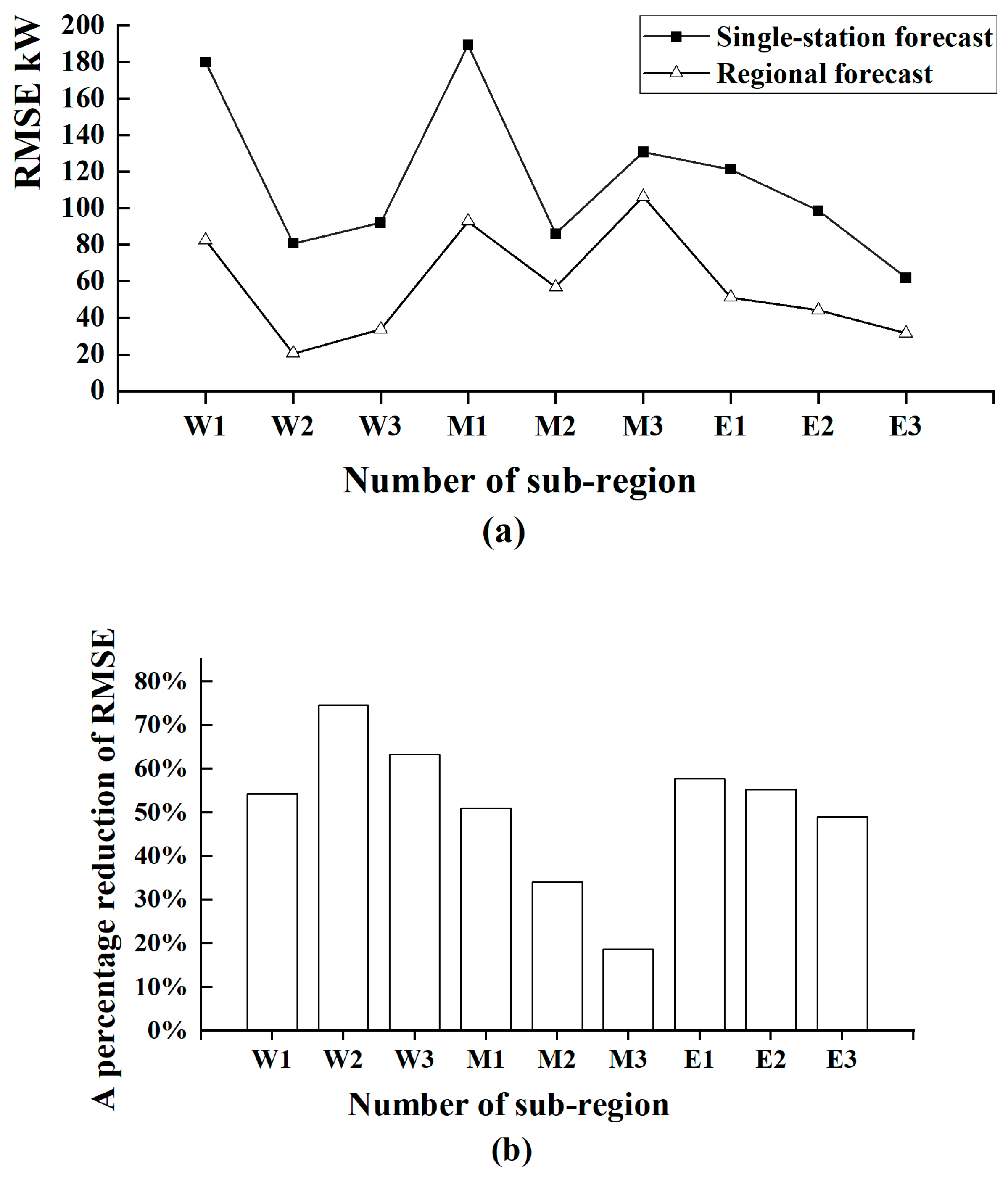
3.1. Effectiveness of Regional Forecasting

The medium- and long-term forecast of wind power in northern Xinjiang was used as an example, to verify the effectiveness of the method proposed in this paper. As shown in Figure 2, there are 11 observation stations in northern Xinjiang. After analysis, the wind power of the 11 observation points in this area showed a high similarity, and they were regarded as one area for forecasting.

In this paper, the root-mean-square-error (RMSE) evaluation index was used to evaluate the forecast performance. In

Table 1. Comparison of the site and area forecast error (kW).

Station Position	1	2	3	4	5	6	7	8	9	10	11	Average Value
Single-station forecast error (kW)	255	314	126	217	073	245	147	362	27	104	110	180
Regional forecast error (kW)	82

, the RMSE values of forecasting directly using the LSTM method for a single station and the whole region are listed.

As can be seen from Table 1, the forecast error for each station individually was relatively large, with RMSE values ranging from 27 to 362 kW and an average value of 180 kW, while the forecast error for the whole region was relatively small, with an RMSE value of 82 kW, which was reduced by 54.20%. This indicated that the medium- and long-term wind-power forecast method based on regional similarities proposed in this paper can reduce the forecast error and improve the forecast accuracy of medium- and long-term wind-resource forecasts.

Figure 3 shows the individual forecast results of No. 2 station in northern Xinjiang, and the region-coupling forecast results of the whole area. The forecast and measured results from January 2011 to December 2016 are listed below.

It is also clear from Figure 3 that the deviation in single-station forecast results was relatively large, especially from January 2015 to December 2016, and the deviation in the forecasted wind power from the measured wind power ranged from 5.20 to 628.32 kW. However, the deviations in the region-coupling forecasting results were smaller, ranging from 1.58 to 198.17 kW, which again illustrated the effectiveness of the method proposed in this paper.

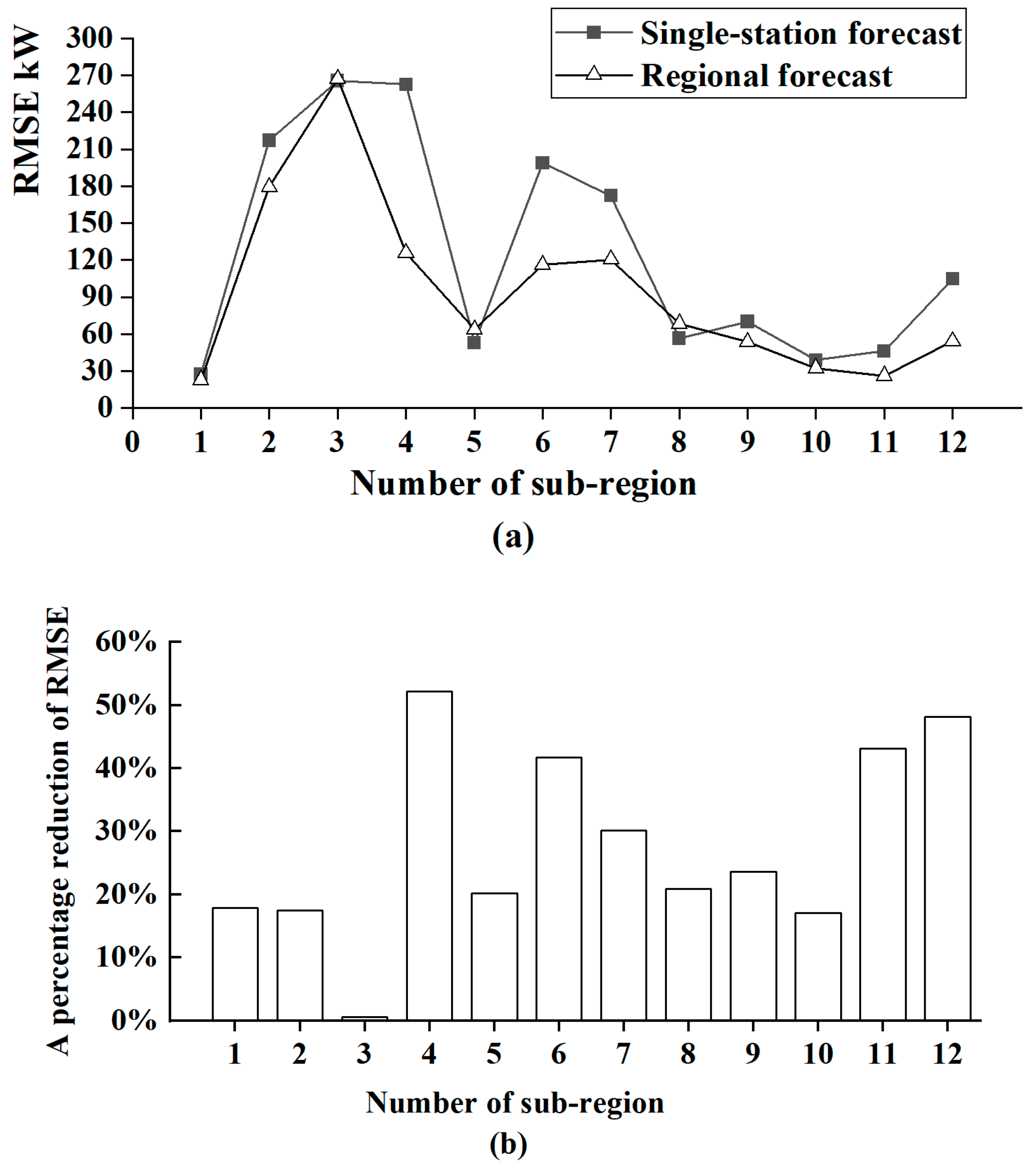
3.2. Large-Area Division and Forecasts

Influenced by terrain and other conditions, wind resources will show certain spatial differences, and the larger the range, the greater the difference. In the five provinces of Northwest China, the provinces bounded by the Arjinshan and Qilian Mountains, the wind resources in the southern and northern regions show relatively different characteristics. In view of this, this paper divided the study area into nine large areas, West 1 to 3, Middle 1 to 3, and East 1 to 3, considering the characteristics of the different altitude, terrain, and location where the five provinces of Northwest China are located, as shown in Figure 4.

The LSTM-based medium- and long-term forecasts of wind power were carried out for individual sites and for the whole region, according to the nine sub-regions divided in Figure 4, and Figure 5 shows the RMSE of the forecast and the improvement rate in the regional-forecast accuracy.

As can be seen from Figure 5, the RMSE (the average value of the RMSE of all single-station forecasts in the sub-region) for the nine sub-regions ranged from 61.98 to 189.37 kW, while the RMSE of the regional forecast was smaller, ranging from 20.50 to 106.38 kW, with a percentage-reduction range of 18.64% to 74.59%. The average RMSE value is reduced from the original 115.64 kW to 57.73 kW, with an average percentage reduction of 50.86%. The average values of the single-station forecast RMSE in the western, central, and eastern regions of the five provinces of Northwest China were 117.58 kW, 135.36 kW and 93.97 kW, respectively; the average regional-forecast-RMSE values were 45.56 kW, 85.30 kW, and 42.32 kW, respectively. The improvement rates were 64.04%, 34.53%, and 54.01%, respectively.

3.3. Small-Area Classification and Forecasting

There were the large differences in wind-resource characteristics between different terrains (such as plains, hills, and mountains), which, on the one hand reflect the differences between wind-resource regions, while on the other hand, wind resources presented better similarity and characteristics in a specific spatial range in years with high wind speed (hereinafter referred to as windy years). Combining terrain differences and wind-resource similarities in windy years can refine the area division, divide the five provinces of Northwest China into several small areas, and allow medium- and long-term wind-power forecasting to be carried out.

The sub-region division process and results were as follows. In the first step, the five provinces of Northwest China were divided into 153 small areas, using the Thiessen-polygon method, according to the location of the meteorological stations, as shown in Figure a. In the second step, the local terrain of the small areas to which the meteorological stations belonged was considered comprehensively (plains, hills, mountains), as well as the ladders (first and second ladders). From this, 153 small areas could be divided into six terrain categories, as shown in Figure 6b. In the third step, small tracts of the same terrain category adjacent to each other were merged, resulting in 40 sub-regions, as shown in Figure 6c. In the fourth step, 153 small areas were categorized according to the similarity of the multi-year monthly average-wind-power-trend time series of high-wind years (see 1.2.2 for details of the calculation method), and six similar categories were obtained, the results of which are shown in Figure 6d. Finally, superimposing and merging the results of terrain category and similar category classification in Figure 6c,d, 12 sub-regions were obtained, as shown in Figure 7.

The RMSE results are shown in Figure 8 for each sub-region, based on the results of the zoning in Figure 6, and the medium- and long-term forecast of wind power for individual sites and the whole sub-region, respectively. As can be seen from Figure 7, the average RMSE of the 12 sub-regions ranged from 27.77 to 265.66 kW for the single-station forecasts, while the RMSE of the regional forecast ranged from 22.82 to 267.19 kW, and the error for the latter was reduced from −20.86% to 52.16%, compared with the former. For the 12 sub-regions as a whole, the average RMSE was also reduced, from 126.16 kW for the single-station forecast to 94.15 kW, with an average reduction of 20.80 kW to 94.15 kW for the 12 sub-regions as a whole.

Comparing the forecast results of large areas and small areas, both improved the forecast accuracy compared with single-station forecasts, but the improved forecast accuracy was different for each. It can be seen that different methods of zoning will affect the accuracy of regional forecasts. Due to limitations of terrain and geomorphological information, the study did not conduct further research on the zoning of other factors.

4. Conclusions

Considering the deficiency of single-site wind-power forecasting, and the availability of regional characteristics of wind power, this paper proposes a medium- and long-term wind-power-trend forecast method based on regional similarities, and gives specific steps for similarity identification and regional division. A case study was carried out in Northwest China, and the following conclusions were obtained:

• The proposed method was effective. Compared with the single-station forecast, the forecast error was significantly reduced, and the mean value of RMSE was reduced by 20%, on average. The forecast accuracy is improved.
• The approach of area division had a certain impact on the accuracy of the regional forecast, which will be studied in the future.

The conclusions proved that the proposed method was viable, and the regional characteristics could be used to improve the accuracy of the wind forecasts. However, some limitations are worth noting. The proposed method in this paper only considered regional similarities, without the density of measurement stations; moreover, the wind-shear index was a composite of all or part of the wind-measurement data. Future work will focus on the accurate delineation of terrain, and the wind-shear index which depends on the atmospheric stability will be studied.

References

1. Han, Z.; Jing, Q.; Zhang, Y.; Bai, R.Q.; Guo, K.M.; Zhang, Y. Review of wind power forecasting methods and new trends. Power Syst. Prot. Control 2019, 47, 178–187. [Google Scholar]
2. Zhang, H.Y.; Ding, Y.G.; Liu, M.; Yang, H.Q.; Zhang, B. Numerical simulation of wind energy resources distribution in Hubei province. Meteorol. Environ. Sci. 2008, 138, 35–38. [Google Scholar]
3. Peijun, S.; Gangfeng, Z.; Feng, K.; Qian, Y. Wind speed change regionalization in China in 1961–2012. Progress. Inquisitiones Mutat. Clim. 2015, 11, 387–394. [Google Scholar]
4. Ding, C.X.; Yan, J.P.; Li, M.M. Climate change and response characteristics to wind speed in northwestern China. Bull. Soil Water Conserv. 2014, 34, 134–137. [Google Scholar]
5. Luo, W.; Cui, N.; Zhang, Q.; Feng, Y.; Gong, D.; LV, M. The spatial and temporal characteristics and causes of meteorological factors in Northwest China in recent 50 years. China Rural Water Hydropower 2018, 431, 12–19. [Google Scholar]
6. Sun, S.; Dong, C.; Wang, Z.; Jiang, J.; Zhang, Y. Medium- and long-term quantity of electricity forecasting method in wind power considering different wind energy characteristics. High Volt. Eng. 2021, 47, 1224–1233. [Google Scholar]
7. Xu, Y. Research of the Methods of Medium- and Long-Term Wind Power Forecasting; Shenyang Institute of Engineering: Shenyang, China, 2017. [Google Scholar]
8. Dang, R.; Zhang, J. Wind Power Prediction Based on Auto-regressive and Moving Average Model. J. Anhui Univ. Technol. (Nat. Sci.) 2015, 32, 273–277. [Google Scholar]
9. Kusiak, A.; Zhang, Z. Short-horizon prediction of wind power: A data-driven approach. IEEE Trans. Energy Convers. 2010, 25, 1112–1122. [Google Scholar] [CrossRef]
10. Abdel-Karim, N.; Small, M.; Ilic, M. Short term wind speed prediction by finite and infinite impulse response filters a state space model representation using discrete markov process. IEEE Buchar. Power Tech. Conf. 2009, 13, 1–8. [Google Scholar]
11. Bessa, R.J.; Miranda, V.; Gama, J. Entropy and correntropy against minimum square error in offline and online three-day ahead wind power forecasting. IEEE Trans. Power Syst. 2009, 24, 1657–1666. [Google Scholar] [CrossRef]
12. Gao, S.; Dong, L.; Gao, Y.; Liao, X. Medium- and long-term wind speed prediction based on rough set theory. Proc. CSEE 2012, 32, 32–37. [Google Scholar]
13. Wang, W.; Liu, H.; Chen, Y.; Zheng, N.; Li, Z.; Ji, X.; Yu, G.; Kang, J. Wind power forecast based on LSTM cyclic neural network. Renew. Energy Resour. 2020, 38, 1187–1191. [Google Scholar]
14. Preeti, R.B.; Singh, R.P. Financial and Non-Stationary Time Series Forecasting using LSTM Recurrent Neural Network for Short and Long Horizon. In Proceedings of the 2019 10th International Conference on Computing, Communication and Networking Technologies (ICCCNT), Kanpur, India, 6–8 July 2019; pp. 1–7. [Google Scholar] [CrossRef]
15. Wang, Y.; Liang, Q.; Zhang, S.; Liu, E.; Huang, Y. An Ultra-short-term Wind Power Prediction Method Based on LSTM-XGboost Combination. Sci. Technol. Eng. 2022, 22, 5629–5635. [Google Scholar]
16. Han, S.; Qiao, Y.H.; Yan, J.; Liu, Y.Q.; Li, L.; Wang, Z. Mid-to-long term wind and photovoltaic power generation prediction based on copula function and long short term memory network. Appl. Energy 2019, 239, 181–191. [Google Scholar] [CrossRef]
17. Zhang, H. Research on Spatial-Temporal Uncertainty Prediction Method of Wind Power; North China Electric Power University: Beijing, China, 2021. [Google Scholar]
18. Lu, J.; Wang, Y.; Yang, Y.; He, Z.; Xiang, L.; Li, X. Wind Power Short-term Prediction Based on the Long-term Memory Model the Time Series Analysis Method. Sci. Technol. Eng. 2015, 15, 50–55. [Google Scholar]
19. Shan, B.; Li, H.; Gu, R.; Li, L. Short-term Wind Power Combination Prediction Based on Beetle Antennae Search Algorithm. Sci. Technol. Eng. 2022, 22, 540–546. [Google Scholar]
20. Li, H. Analysis of the Temporal and Spatial Variation of Wind Shear Index in China; Lanzhou University: Lanzhou, China, 2016. [Google Scholar]
21. GB/T 18710-2002; Wind Energy Resource Assessment Method for Wind Farms. General Administration of Quality Supervision, Inspection and Quarantine of the People’s Republic of China: Beijing, China, 2002.
22. DL/T 5240-2010; Technical Regulations for Design and Calculation of Thermal Power Plant Combustion System. GB Electric Standards: Beijing, China, 2010.
23. Cao, Y.; Yan, S.; Liu, H.; Guo, L. Short-term wind power forecasting method based on noise-reduction time-series deep learning network. Proc. CSU-EPSA 2020, 32, 145–150. [Google Scholar]
24. John, F.E.; Ric, W. Fractal dimension as a market mode sensor. Tech. Anal. Stock. Commod. 2010, 28, 16–20. [Google Scholar]
25. Gurrib, I.; Elshareif, E. Optimizing the performance of the fractal adaptive moving average strategy: The case of EUR/USD. Int. J. Econ. Financ. 2016, 8, 171–178. [Google Scholar] [CrossRef] [Green Version]
26. Wang, X.; Mei, Y. Flood Process Similarity Analysis Method and System Based on Centroid Process Line. CN Patent CN201410284732.8, 3 September 2014. [Google Scholar]
Figure 1. A flowchart of the proposed method.
Atmosphere 14 00430 g001
Figure 2. Sketch map of wind-speed observation station in northern Xinjiang.
Atmosphere 14 00430 g002
Figure 3. Comparison of site and area forecasts: (a) The forecast results of No. 2 station; (b) The forecast results of coupling region.
Atmosphere 14 00430 g003
Figure 4. Results of the large-area division of the northwest region.
Atmosphere 14 00430 g004
Figure 5. Forecast results based on large-area partition (a,b).
Atmosphere 14 00430 g005
Figure 6. The process of small-area classification in northwest China. (a) Thiessen Polygon; (b) Terrain classification; (c) Terrain classification merged; (d) Classification of windy-year similarity.
Atmosphere 14 00430 g006aAtmosphere 14 00430 g006b
Figure 7. Result of sub-region division considering terrain differences and similarity of wind resources.
Atmosphere 14 00430 g007
Figure 8. Forecast results based on small-area partition (a,b).
Atmosphere 14 00430 g008