
Atmospheric Instability and Its Associated Oscillations in the Tropics

DEVCOM Army Research Laboratory, Adelphi, MD 20783, USA
Atmosphere 2023, 14(3), 433; https://doi.org/10.3390/atmos14030433
Submission received: 10 January 2023
/
Revised: 13 February 2023
/
Accepted: 16 February 2023
/
Published: 21 February 2023
(This article belongs to the Special Issue 50th Anniversary of the Metaphorical Butterfly Effect since Lorenz (1972): Multistability, Multiscale Predictability, and Sensitivity in Numerical Models)
Abstract
:The interaction between tropical clouds and radiation is studied in the context of the weak temperature gradient approximation, using very low order systems (e.g., a two-column two-layer model) as a zeroth-order approximation. Its criteria for the instability are derived in the systems. Owing to the connection between the instability (unstable fixed point) and the oscillation (limit cycle) in physics (phase) space, the systems suggest that the instability of tropical clouds and radiation leads to the atmospheric oscillations with distinct timescales observed. That is, the instability of the boundary layer quasi-equilibrium leads to the quasi-two-day oscillation, the instability of the radiative convective equilibrium leads to the Madden–Julian oscillation (MJO), and the instability of the radiative convective flux equilibrium leads to the El Niño–southern oscillation. In addition, a linear model as a first-order approximation is introduced to reveal the zonal asymmetry of the atmospheric response to a standing convective/radiative heating oscillation. Its asymmetric resonance conditions explain why a standing ~45-day oscillation in the systems brings about a planetary-scale eastward travelling vertical circulation like the MJO. The systems, despite of their simplicity, replicate the oscillations with the distinct timescales observed, providing a novel cloud parameterization for weather and climate models. Their instability criteria further suggests that the models can successfully predict the oscillations if they properly represent cirrus clouds and convective downdrafts in the tropics.
1. Introduction
The views of atmospheric predictability changed from Laplace’s determinism to the deterministic chaos of Lorenz (1963), and recently to the coexistence of determinism and chaos (Shen et al. 2021; see Shen et al. 2022 for review) [1,2,3]. Since the previous studies focused on the Bénard convection and the geostrophic baroclinic model in the middle latitudes (Lorenz 1963, 1969, 1990) [1,4,5], the present study focuses on tropical convection, the engine of atmospheric circulations (Riehl and Malkus 1958) [6].
Lorenz (1963) used a nonlinear system of three differential equations to study the predictability of dry convection with a timescale of minutes [1], referring to the predictability of weather and climate change. Since the Lorenz system included a convective instability, its prognostic variables changed periodically and/or non-periodically. Once the system had no instability, its prognostic variables eventually became steady, which exhibited the importance of the convective instability in the predictability.
In this paper, simple systems like the Lorenz system were constructed to address the predictability of weather and climate change in the tropics. The systems incorporated two key components of weather and climate change: moisture (or clouds), which involves the release of potential energy and radiation, which controls the generation of potential energy and is affected by the clouds. In addition, the systems use the instability of tropical clouds and large-scale circulation (Raymond and Zeng 2000) in place of the convective instability in the Lorenz system, where the instability of Raymond and Zeng (2000) has a much longer timescale than the convective instability (see Section 2) [7].
In the proposed systems, the instability was usually connected to oscillations, where one of them is illustrated as
where X2 and Y2 represent the dimensionless air surface entropy (or energy) in one region and the air saturation moist entropy (or temperature) at an altitude of 2 km in another neighboring region, respectively. The system of Equation (1) describes the charge and discharge of entropy in the planetary boundary layer (PBL) (see Appendix C for details). It has an unstable fixed point of X2 = Y2 = 0 in the phase space (X2, Y2), which corresponds to the instability of the boundary layer quasi-equilibrium. It also has a limit cycle that corresponds to a quasi-two-day oscillation (see Figure 1). Once its coefficients are changed so that the fixed point becomes stable, its limit cycle expires. This connection between the unstable fixed point and the limit cycle is generalized to all the continuous dynamical systems on the plane by the Poincaré—Bendixson theorem [8], suggesting that the quasi-two-day oscillation is connected to the instability of the boundary layer quasi-equilibrium.
The instability of the boundary layer quasi-equilibrium in the system functions similarly to the convective instability in the Lorenz system, and, therefore, is key to understand the quasi-two-day oscillation. In this paper, the connection between the instability and the oscillation is extended to other two cases: the Madden–Julian oscillation (MJO) and the El Niño–southern oscillation (ENSO).
The paper is organized as follows. Section 2 uses the moist entropy to distinguish two opposite views on convective clouds and large-scale circulations. Section 3 illustrates the instability of the radiative convective equilibrium in the context of the weak temperature gradient approximation. Section 4 introduces a two-column two-layer model of the interaction between tropical clouds and large-scale circulations. Section 5 extends the model to the other two cases with distinct timescales observed. Section 6 concludes the paper.
2. Are Convective Clouds Active or Passive?
There are two opposite views on atmospheric convection in the tropics. Deep convective clouds, as an active factor, penetrate through the level of the minimum moist entropy into the upper troposphere (UT) as hot towers and subsequently drive large-scale vertical circulations (e.g., the Hadley circulation, hurricanes) (Riehl and Malkus 1958) [6]. On the other hand, convective clouds occur as a passive factor to balance atmospheric radiation losses and consequently their spectrum is controlled by radiative cooling (Manabe and Strickler 1964) [9]. In this section, the two opposite views are distinguished via a series of ideal experiments on the radiative convective equilibrium (RCE), beginning with the expression of the moist entropy.
2.1. Expression of Moist Entropy
Consider an air parcel with water vapor, liquid drops and ice particles. Its moist entropy per unit mass of dry air equals the sum of the entropy of dry air and the entropies of vapor, liquid and solid water. The moist entropy thus is expressed as [10]
where T is the air temperature, p is the total pressure of the moist air, e is the partial pressure of the water vapor, qt is the total mixing ratio of the airborne water (i.e., qt = qv + qc + qi), qv/qc/qi is the mixing ratio of the water vapor/cloud water/cloud ice, Lv/Lf is the latent heat of the vaporization/freezing, Cp/cl is the specific heat of the dry air/liquid water, Rd/Rv is the gas constant of the dry air/water vapor, Esw/Esi is the saturation vapor pressure over water/ice and f = e/Esw is the relative humidity of the air. In addition, Tref = 273.15 K and pref = 105 pa are the reference temperature and pressure, respectively.
When an air parcel ascends or descends adiabatically, its moist entropy changes with time t as
where Qs represents the increase in entropy from the irreversible processes (e.g., the heat flow from high to low temperature, liquid drop evaporation and ice particle melting; see [10] for its expression). When Tref = 273.15 K (i.e., at the triple point of pure water), Qs is small. Hence Qs ≈ 0 (or the conservation of moist entry) is usually assumed in a conceptual model.
The moist entropy is related to the equivalent potential temperature θse by s = Cpln(θse/Tref) [11]. It functions similar to the moist static energy (or CpT + gz + Lvqv where z is the height and g is the acceleration due to gravity), although the moist static energy is not conserved in the convective regions with a strong vertical velocity. In addition, Equation (3) can be used to simulate an air parcel with the same accuracy as the energy equation represented in terms of the (potential) temperature [12].
The moist entropy yields conceptual models of atmospheric convection [6]. In contrast, other variables (e.g., temperature or its variation) often yield ill-posed models by artificially separating the water and energy cycles in the atmosphere. One ill-posed model, for example, is the convective instability of the second kind (CISK) [13], which is reasoned as follows. Consider a horizontally uniform atmosphere with convective available potential energy (CAPE). No matter how large the low-level horizontal convergence is and the strength of the convective clouds it induces, the mid-tropospheric temperature never surpasses the temperature of an air parcel that moves adiabatically from the surface to the middle troposphere. In other words, the mid-tropospheric temperature has an upper limit, which is contrary to the prediction of the unlimited mid-tropospheric temperature in the CISK [14,15]. Since the moist entropy does not need an artificial separation of the water and energy cycles, it cannot yield an ill-posed model of moist convection like the CISK.
2.2. Approach of the RCE
Consider a tropical atmosphere subject to radiative cooling over the oceanic equator. Since the radiative cooling brings about the CAPE, convection occurs and transports the energy upward, leading to a balance between the radiative cooling and the convective heating, which is referred to as the RCE [16,17,18,19].
The RCE has three forcing factors: the radiative cooling rate, air surface wind speed and sea surface temperature (SST). If the forcing factors are fixed, coupling does not occur between the convection, atmospheric radiation and surface wind in the atmosphere, providing a simple case to determine the timescales in the approach of the RCE.
Suppose that the radiative cooling rate is 1 °C/day below the height z = 9 km and decreases linearly with height to zero at z = 15 km. In addition, the surface wind speed = 4 m s−1 and the SST = 302 K are set, which are used for determining the sensible heat flux from the sea to the air and the latent heat flux due to sea surface evaporation.
The RCE is simulated with a cloud resolving model (CRM), using the periodic lateral boundary conditions and the vertical velocity w = 0 at the sea surface [19]. Figure 2 displays the time series of the three modeled variables: the flux of entropy from the sea to the air due to sea surface evaporation and the sensible heat transfer from the sea to the air, the flux of entropy from the air to space due to the radiative cooling, and the internal generation of entropy due to cloud microphysics (e.g., rainwater evaporation) and the heat transfer from high to low temperature (or mixing). In the figure, the surface entropy flux from the sea to the air approaches the top entropy flux from the air to space, arriving at the RCE eventually, where the internal entropy generation is negligible.
Figure 3 displays the time series of the air temperature and the relative humidity at z = 0 and 4.5 km, showing two timescales of the temperature in the approach of the RCE. The short timescale is ~2 days and is associated with the timescale of the relative humidity. Hence, the short timescale measures the approach of the water quasi-balance between the sea surface evaporation and precipitation (figure omitted). In contrast, the long timescale measures the approach of the RCE while the atmosphere remains at the water quasi-balance.
The long timescale of the temperature = 29.2 days, obtained by fitting the mid-tropospheric temperature after day four in Figure 3 with , is explained with the budget equation of the tropospheric entropy. Consider a small perturbation of the troposphere from the RCE whose deviation of the moist entropy of the air at z = 0 is denoted as . Thus, represents the deviation of the total entropy of the troposphere, where and are the pressure at the sea surface and tropopause, respectively; and μ is the vertically averaged deviation of the moist entropy relative to that at z = 0. After overlooking the internal generation of entropy, the budget equation of the moist entropy of the troposphere becomes
where the first and second terms on the right-hand side represent the surface and top entropy fluxes, respectively; is the air density near the sea surface, = 1.1 × 10⁻³, is the surface wind speed, is the entropy of the sea surface water as a function of the SST, is the surface moist entropy at the RCE; and FR is the entropy flux from the air to space due to radiative cooling.
Since the top and surface entropy fluxes are balanced at the RCE or , Equation (4) is solved with , where the following timescale
shows that is inversely proportional to .
The CRM simulations support the inverse relationship between and the surface wind speed [19]. Figure 4 displays the modeled against the dimensionless number
where is the total loss of energy of the troposphere due to radiative cooling. The figure also displays the theoretical timescale estimated with Equation (5) and μ = 3.6 for comparison. Generally speaking, Equation (5) agrees with the CRM results except at some low values of Nw ~100 where the initial status is so close to the RCE that the long timescale in the approach of the RCE is not clear and, consequently, its estimation is “polluted” by the short timescale.
In addition, the modeled decreases with an increase in the radiative cooling rate, which is attributed to the sensitivity of μ to the radiative cooling rate. If the CAPE = 0 were maintained strictly, μ = 1. However, convection usually lags the generation of the CAPE, bringing about μ ≠ 1. When the radiative cooling rate varies with a very short forcing period, for example, μ >> 1 because the surface entropy does not have sufficient time to respond to the cooling of the troposphere. The CRM simulations show that at the radiative cooling rate of 2 °C/day is about one half of that at the radiative cooling rate 1 °C/day [19]. Hence, μ = 1.8 at the radiative cooling rate of 2 °C/day is obtained that is about one half of μ = 3.6 at the radiative cooling rate 1 °C/day.
2.3. Ideal Experiments of the RCE
To show whether the convective clouds are active or passive, two ideal experiments of the RCE were designed with prescribed forcing. The first experiment used a fixed radiative cooling rate of
where is the mean surface wind speed, A is the dimensionless amplitude and ω is the angular frequency of the forcing. Substituting Equation (7) for Equation (4) and then solving the resulting equation yields
and the surface entropy flux with the aid of Equation (5).
Figure 5 displays the amplitudes of the air surface temperature and the surface energy flux from Equation (8) against the forcing period of the surface wind. For the forcing period 2π/ω << , Equation (8) degenerates into the term of , which is referred to here as the active mode. In this mode, leads to a sine variation of the surface entropy flux and a cosine variation of the surface moist entropy (or the CAPE). The convective clouds then distribute the cosine variation of the surface moist entropy into the mid-troposphere, bringing about a cosine variation of the mid-tropospheric moist entropy (or temperature). Hence, the convective clouds are active, leading to the variation of the mid-tropospheric moist entropy (or temperature).
For 2π/ω >> , Equation (8) degenerates into the term of 2sin(ωt), which is referred to as the passive mode. In this mode, the atmosphere is always close to the RCE and, thus, the surface entropy flux is controlled by the fixed radiative cooling rate. Since the surface entropy flux or is constant, is inversely proportional to . As a result, the surface entropy changes with but the surface entropy flux does not, indicating that the convective clouds are passive and controlled by the radiative cooling rate.
As a general case, Equation (8) possesses both the active and passive modes. When the forcing period 2π/ω is close to or
the two terms of and 2sin(ωt) in Equation (8) have the same amplitude, indicating the active and passive modes have the same importance. Their relative importance is measured by the phase delay of the variation in the mid-tropospheric entropy (or temperature) with respect to the variation in the forcing.
To test the analytic solution of Equation (8), three CRM simulations were carried out [19]. The simulations used the forcing period 2π/ω = 4, 32 and 128 days in Equation (7), respectively. In addition, the simulations set = 6 m s−1, A = 1/3, and the radiative cooling rate at 2 K/day. Their results are displayed in Figure 5, supporting the analytic solution of Equation (8).
The second ideal experiment, in contrast to the first one, was carried out to test the response of the convective clouds to the radiative cooling. The experiment used a fixed surface wind speed , but the radiative cooling rate was
where Qr0(z) equals 1.5 °C/day below the height z = 9 km and decreases linearly with the height to zero at z = 15 km. Substituting Equation (10) for Equation (4) yields
and the surface entropy flux, where FR0 denotes the entropy flux from the air to space with the radiative cooling rate Qr0.
The amplitudes of the air surface temperature and the surface energy flux were computed using Equation (11). They were displayed against the forcing period of the radiative cooling in Figure 6. To support the analytic solution of Equation (11), three CRM simulations were carried out with the forcing period 2π/ω = 4, 32 and 128 days in (10), respectively [19]. In addition, the CRM simulations used = 4 m s−1 and A = 1/3. Their results are displayed in Figure 6 for comparison, supporting the analytic solution of Equation (11).
The second experiment supported the first one regarding the separation between the active and passive modes (see Figure 5 and Figure 6). When the forcing period was long (or 2π/ω >> ), the top entropy flux determined the surface entropy flux whether the surface wind changed or not, indicating the radiative cooling rate controlled the convective clouds. In contrast, when the forcing period was short (or 2π/ω << ), the top entropy flux had almost no effect on the surface entropy flux.
In summary, the active and passive modes were separated at the forcing period of the surface wind and radiative cooling at 2π/ω = π ≈ 45 days (if = 14 days; see Figure 4 for the variation of τt), which corresponds to the period of the MJO [20,21,22]. Roughly speaking, the convective clouds were active in the weather systems with a timescale shorter than ~ 45 days, they are passive in the climate systems with a timescale longer than ~45 days and they possessed dual roles in the systems with a timescale of ~45 days (e.g., the MJO).
3. Instability of the RCE
The RCE in a wide region is unstable once its clouds are organized via a large-scale vertical circulation into two sub-regions: one with deep convective clouds and the other with shallow (or no) clouds (Raymond and Zeng 2000; Sessions et al. 2010) [7,23], which explains the strong Hadley circulation observed (Raymond 2000) [24]. In this section, the instability of the RCE is discussed with its key processes, beginning with its foundation in the weak temperature gradient (WTG) approximation (Bretherton and Smolarkiewicz 1989; Sobel and Bretherton 2000; Bretherton and Sobel 2002) [25,26,27].
3.1. The WTG and Its Application
The WTG is the foundation for understanding the interaction between tropical convection and large-scale vertical circulations (Nilsson and Emanuel 1999; Raymond and Zeng 2000; Sobel and Bretherton 2000) [7,26,28]. In a three-dimensional stratified atmosphere with a large Rossby number (e.g., in the tropics), gravity waves damp the temperature perturbations excited by clouds so that the perturbations disappear eventually, which is referred to as buoyancy damping [19]. On the other hand, the imbalance of the convective heating and radiative cooling generates a forced vertical circulation. Since the horizontal scale of convective clouds is small compared to the Rossby radius of deformation, the amplitude of the forced circulation and the horizontal temperature gradient in the mid-troposphere are small, which is referred to as the WTG [26,27,29]. In brief, buoyancy damping and the WTG represent the process and result of gravity waves, respectively. They are analogous to the damping of the surface waves and the little slope of the pond surface, respectively, when pebbles are tossed into a pond (see Zeng et al. 2020 for the connection between the WTG and buoyancy damping [30]).
Consider two adjacent regions: one with convective clouds and the other with a clear sky. Let Te(z) denote the vertical profile of the temperature in the clear sky (or environment) region and let ΔTe(z) denote the difference in the temperature between the convective region and the clear sky region. Obviously, ΔTe(z) is caused by the imbalance between the convective heating and radiative cooling in the convective region. The analytic model of gravity waves showed that ΔTe(z) was inversely (directly) proportional to the gravity wave phase speed (the heating intensity and the distance between the two regions) [19,31]. Since many gravity waves with different vertical wavelengths (or phase speeds) work at the same time, their ensemble effect on ΔTe(z) can be obtained. Generally speaking, ΔTe(z) is small in the mid-troposphere, working as the WTG. In addition, ΔTe(z) is relatively large and thus the WTG is not suitable in the PBL, indicating the PBL can maintain its local characteristics. Additionally, ΔTe(z) is large in the UT, too, because the tropopause with a strong static stability and the sea surface trap internal gravity waves in the troposphere as two “rigid” boundaries.
3.2. Origin of the Instability
Consider the individual clouds in the convective region. Let denote the temperature of a cloud marked with superscript i. Since represents the difference in the temperature between the two regions, the temperature of cloud i at the mid-tropospheric height is expressed as
Replacing approximately with its ensemble average yields
where the left-hand side has superscript i but the right-hand side does not.
Equation (13) has two different applications. (a) Given the surface entropy , an air parcel near the sea surface ascends adiabatically to the mid-troposphere. Thus, is determined using the entropy conservation and Equation (12). (b) Since the surface entropy below a cloud is changed by the local factors of the cloud itself as well as its neighboring clouds (e.g., convective downdrafts, surface wind gusts), the surface entropy cannot be known at first. Instead, given the right-hand side of Equation (13), is known using the entropy conservation or
where denotes the pressure at the mid-troposphere and s*(T, p) is the saturation moist entropy of the air with temperature T and pressure p (or the entropy of the air that is saturated with respect to water at temperature T and pressure p).
Equation (14) resembles the model of Emanuel et al. (1994) in that the vertical temperature profile itself is controlled by convection and tied directly to the surface entropy [14]. The model of Emanuel et al. (1994) is based on the idea that convection is nearly in statistical equilibrium with its environment or ≈ 0. After taking the WTG (i.e., ≈ 0) and ≈ 0, Equation (14) is approximated as a concept or
That is, the surface entropy in the convective region is determined by the mid-tropospheric temperature in the clear sky region.
Other models of the convective atmosphere in a tropical β channel complement Equation (15) with higher-order accuracy. The first model with Equation (15) in Section 4, as the zeroth-order approximation, produces a small variation of the imbalance between convective heating and radiative cooling and, thus, a small variation of in a region. The second model in Appendix D, as the first-order approximation, represents a global response (i.e., vertical circulations) to the small thermal forcing in the first model. The third model, as the second-order approximation, represents the feedback between the forced vertical circulations and convective clouds especially those beyond the region of the first model.
If a large-scale vertical circulation was not present between the two regions, the atmosphere in the convective region would stay at the RCE with the surface entropy . Since is determined by the convective downdrafts, SST, surface wind and other local factors (see Section 2),
because the right-hand side is determined by a non-local factor, the mid-tropospheric temperature in the clear sky region. The inequality (16) leads to the instability of the RCE. Specifically, the large-scale vertical circulation rises to modulate deep convective clouds that, in turn, change until satisfies Equation (16). In other words, the instability exhibits a movement of from to with a growing large-scale vertical circulation.
3.3. Convective Downdrafts
Convective downdrafts embody the movement of from to by redistributing entropy vertically. Figure 7 displays the vertical profile of the buoyancy of an air parcel that ascends adiabatically from the surface to the UT, where the buoyancy is directly proportional to the difference in entropy between the surface entropy (green/black line) and the saturation moist entropy of the environmental air (red line). During their ascent from the surface to the UT, the air parcels detrain into the UT and then mix with their environment. Since the entropy of the mixed parcels falls between the blue and black lines, the cloud detrainment increases the UT entropy. If some mixed parcels have an entropy between the blue and red lines, their buoyancy becomes negative, forming convective downdrafts. Once the lower tropospheric downdrafts penetrate into the PBL, they bring down the mid-tropospheric air with low entropy into the PBL and, consequently, decrease the surface entropy.
Observations show that convective downdrafts are common in the tropics [32,33,34,35]. Figure 8, for example, displays the vertical distribution of downdrafts in a mature mesoscale convective system (MCS) observed by airborne nadir pointing Doppler radar during the Tropical Composition, Cloud and Climate Coupling (TC4) Experiment [36]. The figure displays the vertical cross sections of the observed radar reflectivity and Doppler velocity using the ER-2 Doppler radar (EDOP) on the NASA high-altitude (~20 km) ER-2 aircraft [37,38]. After taking the fall speed of the hydrometeors (ranging from 2.5 to 10 m s−1 with a reflectivity from 0 to 50 dBZ for the drops; 1.2 to 1.8 m s−1 with a reflectivity increasing from –10 to 30 dBZ for snow and 1.8 to 5.4 m s−1 with a reflectivity from 30 to 45 dBZ for graupel) off the Doppler velocity [37], the figure clearly shows that convective downdrafts, especially those in the lower troposphere, are quite common.
The movement of from to is affected indirectly by a large-scale vertical circulation via deep convective clouds and their downdrafts. To be specific, the large-scale ascent (descent) raises (lowers) the top of deep convective clouds, which is discussed with the aid of Figure 7. A UT large-scale descent brings about an increase in entropy by vertical advection and an increase in the temperature due to the air compression in the UT. As a result, the descent leads to a shift of the blue and red lines in the UT to the right in Figure 7. Since the descent has no impact on the surface entropy (i.e., no impact on the green line in Figure 7), the descent lowers the top of the deep convective clouds (or the height with zero buoyancy). If the descent continues, the deep convective clouds decrease in population and, eventually, shallow ones take their place, which are simulated by the CRM simulations of Sessions et al. (2010) [23]. Similarly, the UT large-scale ascent decreases the UT entropy by vertical advection and, thus, leads to a shift of the blue and red lines in the UT to the left in Figure 7, raising the top of the convective clouds. In short, the large-scale ascent/descent affects the deep convective clouds that in turn vertically redistribute entropy, impacting indirectly.
3.4. Cirrus Clouds and Their Radiation
Cloud radiation, as a complement of the aforementioned dynamical factors, maintains the instability by fueling deep convective clouds. Cirrus clouds, including the cloud anvil from the MCSs, emit infrared radiation into space, bringing about a decrease in the UT temperature and entropy [39]. Meanwhile, the cirrus cloud amount is affected by large-scale vertical velocity. In general, the amount is increased (decreased) by the large-scale ascent (descent) [7]. In addition, the amount is changed indirectly by the large-scale ascent via UT convective downdrafts (see Figure 8 and Figure 9) [40,41,42,43].
The indirect effect of the large-scale ascent on cirrus clouds via UT downdrafts is discussed as follows. Consider an air parcel with super-cooled drops that undergoes a vertical circulation. When the parcel ascends, its temperature decreases first to activate many ice nuclei (IN), and then ice crystals form on the activated IN [44,45]. With the parcel descending, its super-cooled droplets evaporate first and then a part of the ice crystals disappear via sublimation. The sublimation of the ice crystals leaves new solid particles as residues that can be activated at warmer temperatures than the original IN [46,47]. As a result, the parcel has significantly more activated IN than the same parcel with no vertical circulation. In short, the recycling of IN brings about plentiful ice crystals (or activated IN). Roughly speaking, the number of the activated IN depends on the descent distance of convective downdrafts; it increases by 10 times when the descent distance increases by ~0.5 km [41,42,43].
The downdraft-induced activated IN lead to an increase in the ice crystal number, then a decrease in the precipitation efficiency and eventually an increase in cloud anvils (or cirrus clouds) in the UT [41,43]. This process is shown by two CRM simulations in Figure 9: one with a high number concentration of activated IN and the other with a low number concentration. The broad anvil of the MCSs in the CRM simulation with the plentiful activated IN agrees with the field observations, suggesting that the UT convective downdrafts play an important role in cloud anvils.
In summary, UT convective downdrafts are common in a convective region with a large-scale ascent but rare in a clear sky region with a large-scale descent, indicating that large-scale vertical circulation can significantly change the UT cirrus cloud amount via UT downdrafts. Since the cirrus cloud amount changes the radiative cooling of the UT, it modulates the population of deep convective clouds as feedback.
4. A Two-Column Two-Layer Model
A highly simplified model was constructed to assemble the aforementioned processes. In this section, the model is introduced with its structure first, then the criteria for stable RCE and, finally, a connection between the RCE’s instability and a 40-day oscillation of deep convective clouds.
4.1. Model Structure
Consider a two-column two-layer model on the interaction between convective clouds and large-scale vertical circulations in the tropics (see its schematic in Figure 10). The model, similar to Raymond and Zeng (2000) [7], consisted of two adjacent columns: one for testing and the other for reference. For simplicity, the two columns had the same area with width L. They used the same SST and surface wind speed so that the model focused on the interaction between cloud radiation and large-scale vertical circulation. Each column was characterized by two layers: one for the PBL and the other for the UT with cirrus clouds or cloud anvils that detrained from deep convective clouds (i.e., the layer from 7 to 12 km in Figure 7, Figure 8 and Figure 9). The two layers were bridged by deep convective clouds.
The two columns were connected by a large-scale vertical circulation with a mid-tropospheric vertical velocity wm (or −wm) in the test (or reference) column. Suppose the two columns stay at the RCE initially with entropy ss0 in the PBL, su0 in the UT layer and wm = 0. Once a vertical circulation occurs between them, it induces a perturbation of the surface entropy, denoted by Δss (or −Δss) in the test (or reference) column, and a perturbation of the UT entropy, denoted by Δsu (or −Δsu) in the test (or reference) column. Since the perturbation of the total entropy of the two columns was zero, only the entropy budget of the test column is discussed except for specification.
In the test column, wm is associated with the deep convective clouds. To be specific, wm is affected by two factors: Δss + ss0 − s*(Tm, pm) and Δss − Δsu, where s*(Tm, pm) denotes the saturation moist entropy with a mid-tropospheric temperature Tm and a pressure pm. The first factor, Δss + ss0 − s*, represents the average mid-tropospheric buoyancy of the convective clouds (Figure 7). The second factor, Δss − Δsu, represents the deviation of the average UT buoyancy of the convective clouds. Owing to a low water vapor content in the UT, the UT moist entropy is close to the saturation moist entropy (Figure 7) and, thus, can approximately represent its saturation moist entropy. Hence, Δss − Δsu approximately represents the deviation of the average UT buoyancy of the convective clouds.).
When Δss > Δsu, for example, more convective clouds reach the UT than at the RCE and, subsequently, wm > 0. Hence, the mid-tropospheric vertical velocity is expressed as
where H = 12 km is the depth of the troposphere and τc is a timescale to measure the upward transportation of the air mass into the UT induced by the deep convective clouds. The factor of Δss + ss0 − s*(Tm, pm) is key for the model to embody the WTG, because Δss + ss0 − s*(Tm, pm) ≥ 0 represents an essential condition that a cumulus cloud becomes a deep convective cloud.
Deep convective clouds decrease the entropy in the PBL via their downdrafts. Some of the downdrafts penetrate into the PBL (Figure 8) and, thus, bring the mid-tropospheric air with the minimum entropy smin into the PBL (Figure 7). As a result, the vertical entropy flux from the lower troposphere to the PBL is proportional to . Since the deviation of the deep convective clouds from the RCE is proportional to wm, the deviation of the vertical entropy flux from the lower troposphere to the PBL is also proportional to wm. Hence, the entropy budget of the PBL is expressed as
where the three terms on the right-hand side, in turn, correspond to the entropy flux from sea, the horizontal entropy flux from the reference column and the vertical entropy flux from the lower troposphere to PBL. Us represents the horizontal wind speed of environmental air in PBL with respect to the test column. The dimensionless coefficient kd represents the effect of the downdrafts on the surface entropy.
Deep convective clouds transport the surface air with high entropy into UT and consequently increase the entropy. Hence, the entropy budget of the UT layer is expressed as
where the three terms on the right-hand side, in turn, correspond to the horizontal entropy flux from the reference column, the upward entropy flux from the PBL and the entropy flux to space via infrared radiation. Uu represents the UT horizontal wind speed of the environmental air with respect to the test column, and the dimensionless coefficient ku represents the effect of deep convective cores on the UT entropy. σ is the Stefan–Boltzmann constant, Tu is the UT temperature, pm/pt are the pressure of the mid-troposphere/tropopause and Δσc is the deviation of the UT cloud fraction from σc0, the UT cloud fraction at the RCE.
The UT cloud fraction, Δσc +σc0, depends on the detrainment of the deep convective clouds in the UT and the precipitation formation [48]. Suppose σc0 = 0.5. Since 0 < Δσc + σc0 < 1, −0.5 < Δσc < 0.5, hence, the UT cloud fraction is described by
where the two terms on the right-hand side are attributed to the detrainment of deep convective clouds and the sink of cirrus clouds due to precipitation formation, respectively. The dimensionless coefficient kc represents the effect of the detrainment of deep convective clouds on cirrus cloud fraction, and τp is the timescale of the sink of UT cirrus clouds.
4.2. Stability Criteria of the RCE
The two-column two-layer model is simplified into a very low order system of Equations (18)–(20). The system has three prognostic variables: Δss, Δsu and Δσc. It is studied in the phase space (Δss, Δsu, Δσc) similar to Lorenz (1963) [1]. Obviously, the system has a fixed point of the origin in the phase space that corresponds to the RCE, as shown as
Δss = Δsu = Δσc = 0.
The criteria for the stability of the fixed point (or the RCE) are derived in Appendix A. They contained two factors of cloud radiation: the detrainment of deep convective clouds (or kc) and the timescale of cirrus cloud sink (or τp). When the detrainment of deep convective clouds is strong and the cirrus cloud sink is slow, the RCE is unstable. In addition, the criteria also contain the width L of convective region. When L is small (e.g., ~100 km), the RCE is stable; when L is large (e.g., ~3,000 km), then the RCE is unstable. In other words, the criteria predict that the RCE is unstable over a wide convective region where the horizontal exchange in entropy between the columns is negligible.
4.3. Oscillation and an Unstable RCE
A specific case with an unstable RCE is discussed in Appendix A, where L = 3,000 km and τp = 10 days. Once its initial status was slightly away from the RCE, its status deviated from the RCE permanently and eventually approached a limit cycle (see Figure A1). In addition, its prognostic variables (e.g., surface entropy) oscillated with a period of 40 days (Figure 11). Since the peak of the UT cloud fraction corresponded to the onset of deep convective clouds, Figure 11 shows that the deep convective clouds also oscillated in number with a period of 40 days, providing a prototype of the MJO.
If L is decreased to 100 km, the RCE becomes stable and the oscillation disappears, indicating that the instability of the RCE is an essential condition of the oscillation. If τp is decreased from 10 to 5 days while maintaining L = 3,000 km, the RCE is still unstable, but the oscillation disappears. The system, instead, approaches a steady state where one column shows a large-scale ascent and deep convection and the other shows a large-scale descent and shallow clouds, which resemble the model of Raymond and Zeng (2000) [7]. This sensitivity of the system target to τp (or bifurcation in the phase space) indicates that the slow sink of UT cirrus clouds is another essential condition of the oscillation.
Recently, Zeng et al. (2022) showed the possibility of a slow sink of cirrus clouds in the tropics with a new precipitation process—the radiative effect on microphysics [48]. Consider relatively large ice crystals near cloud top. Owing to their radiative cooling, they grow to precipitating particles at the expense of small ones and then fall off their parent clouds. As a result, thick cirrus clouds (detrained from deep convective clouds) quickly become thin with a timescale of hours. Once the thin cirrus clouds form, their ice crystals undergo radiative warming (see Figure 3 of Zeng et al. 2022 [48]) and, consequently, survive with a slow gravitational deposition of ice crystals and/or a slow crystal sublimation in a large-scale descent.
The surface wind, of course, can be incorporated into the two-column model to represent its effects on the instability and the oscillation (Fuchs and Raymond 2005, 2017; Emanuel 2020; Wang and Sobel 2022) [49,50,51,52]. It is related to a large-scale vertical circulation via the surface wind gusts driven by cloud systems (see Section 5.1) and large-scale surface wind [50,53,54,55].
5. Other Forms of Instability
Instability behaves differently when its timescale is much shorter or much longer than ~45 days. In this section, the two-column two-layer model was extended to two cases with a timescale ~2 days and ~2 years, respectively. To minimize its complexity, the model was tuned for each case by adding or deleting processes.
5.1. Boundary Layer Quasi-Equilibrium
The boundary layer quasi-equilibrium was proposed to describe the quasi-balance in the entropy flux between the surface and the PBL top (Emanuel 1995; Raymond 1995) [56,57]. It arrives with a timescale of ~1 day (or the short timescale of the temperature and relative humidity in Figure 2 and Figure 3). This subsection deals with the instability of the quasi-equilibrium in the context of the WTG, beginning with CRM simulations.
Consider a two-column model that represents clouds in each column with a three-dimensional CRM [19]. The two columns take the same forcing factors (e.g, the SST, radiative cooling rate) similar to the experiment in Figure 2 and Figure 3, except for maintaining the WTG via a large-scale vertical circulation between them. Surprisingly, the model replicates a quasi-two-day oscillation, such as those observed in the western Pacific [58,59,60,61].
To show how the oscillation works, Figure 12 displays the modeled time series of the surface entropy and the entropy flux from the sea to the air. In the test column with the large-scale ascent, the deep convective clouds spend and, thus, rapidly decrease the surface entropy while the sea slowly supplies entropy to the PBL.
The time series in Figure 12 are explained by the evolution of the horizontally averaged surface wind speed and the entropy flux at the PBL top in Figure 13. In the test column, the deep convective clouds generated strong surface gusts and subsequently increased the entropy flux from the sea to the air, providing energy to maintain the deep convective clouds. On the other side, in the reference column with the large-scale descent, few to no deep convective clouds brought about the small upward entropy flux at the PBL top and subsequently a high surface entropy. Once the surface entropy in the reference column becomes very high, deep convective clouds occur and, subsequently, invert the large-scale circulation between the two columns. Hence, the modeled two-day oscillation can be treated as an alternation of the charge and discharge of entropy in the PBL.
In the modeled two-day oscillation, the surface wind gusts induced by convective downdrafts changed the entropy flux from the sea to the air, bringing about the deviation of the boundary layer quasi-equilibrium, which resembled the wind-induced surface heat exchange (WISHE) model (Emanuel 1986; Rotunno and Emanuel 1987; Yano and Emanuel 1991) [53,54,55], to some extent. On the other hand, the population of convective downdrafts depended on the population of deep convective cores that, in turn, depended on the buoyancy at the cloud base. Generally speaking, the higher the buoyancy at the cloud base, the more deep convective cores were initiated, given the same external perturbations. Figure 14 displays the vertical profiles of the moist entropy and the saturation moist entropy near the MCS shown in Figure 8. An ascending surface air parcel, as shown by Figure 14, had a strong negative buoyancy at ~2 km, which explained the lack of scattered convective cores around the MCS.
To explain the modeled oscillation, the two-column two-layer model was modified based on the CRM simulation of Figure 12 and Figure 13. The modified model represents the surface wind gusts by introducing Δws (or −Δws), the deviation of the surface wind speed from ws0 the surface wind speed at the RCE in the test (or reference) column. Since Δws changes the entropy flux from the sea to the PBL, the PBL entropy budget in the test column (18) becomes
where HPBL is the depth of the PBL.
To complement the thermodynamic Equation (22), the model introduced a dynamic equation on ΔT2km, the deviation of the temperature or , the deviation of the saturation moist entropy from the RCE at z = 2 km in the reference column, where corresponds to the peak of red line at z = 2 km in Figure 14. Since is a function of ΔT2km, differentiating Equation (2) with respect to time yields
with the aid of the Clausius—Clapeyron equation, where qvs is the saturation mixing ratio of water vapor at temperature T2km and pressure p2km. In addition, ΔT2km is proportional to (Γd− Γs)/2 times the large-scale vertical velocity at z = 2 km, where Γd and Γs denote the dry and saturated adiabatic lapse rates in the reference and test columns, respectively. Thus, Equation (23) is simplified to
where b1 is the ratio between the large-scale vertical velocities at z = 2 km and the mid-troposphere.
Clearly, represents the average buoyancy of the convective clouds at z = 2 km in the test column and, therefore, approximately describes whether the surface parcels can pass the lifted condensation level to form clouds. Hence, the large-scale vertical velocity at the mid-troposphere is related to by
Since the deep convective clouds generate downdrafts that, in turn, generate surface wind gusts, Δws is directly proportional to wm (see Figure 13), which is expressed as
where b2 is a dimensionless coefficient. In addition, Δsu = 0 is set for simplicity because the radiative cooling slightly impacts the boundary layer quasi-equilibrium (see Section 2.3).
The system of Equation (22) and Equation (24) has a fixed point of = 0 in the phase space that corresponds to the boundary layer quasi-equilibrium. The criteria for the stability of the fixed point of the origin are derived in Appendix C. The criteria showed that the boundary layer quasi-equilibrium is unstable when b2 is large (or the downdraft-induced surface gusts are strong), which is supported by the CRM result in Figure 13. The criteria also show that the boundary layer quasi-equilibrium is unstable when L is large (or over a large convective domain), which is supported by the modeling of the MCS onset in horizontally uniform environments with no wind shear [43,62,63].
A specific case with an unstable boundary layer quasi-equilibrium is discussed in Appendix C, where L = 350 km. Once its initial status was away from the origin, its status deviated from the origin and eventually approached a limit cycle (see Figure 1). In addition, its prognostic variables (e.g., surface entropy) oscillated with a period of 2 days (Figure 15). This standing two-day oscillation can lead to a westward travelling two-day oscillation via the zonal asymmetry of the atmospheric response to the zonally symmetric convective heating (see Appendix D). Hence, the system of Equation (22) and Equation (24) provided a prototype of the observed quasi-two-day oscillation.
5.2. Radiative Convective Flux Equilibrium
Consider a two-column model with the SST as a prognostic variable (Nilsson and Emanuel 1999) [28]. If a large-scale vertical circulation is not present between the two columns, the atmosphere approaches a balance between the radiative cooling, convective heating and surface energy flux in each column, which is referred to as the radiative convective flux equilibrium (RCFE). In contrast to the RCE, the RCFE focuses on the balance between the atmospheric radiative cooling and the surface energy flux, where the surface energy flux is related to the SST that is, in turn, related to the UT cirrus clouds via solar and infrared radiation.
The surface energy flux possesses three timescales: two timescales in the approach of the RCE (see Figure 3) and an additional timescale in the approach of the RCFE. Consider a mixed ocean layer with depth Hmix = 100 m that is situated below the atmosphere. Its thermal capacity is about 25 times as much as that of the atmosphere. Since the atmosphere has a long timescale τt of ~14 days, the surface energy flux has a very long timescale of 25 × 14 = 350 days (or ~1 year) in the approach of the RCFE. This third timescale of ~1 year measures the approach of the RCFE while the atmosphere remains at the RCE.
The two-column two-layer model in Section 4 was extended to incorporate the mixed ocean layer as the third layer (see Figure 10), addressing the instability of the RCFE and its connection to the ENSO [64]. Suppose that the test column sat over the central and eastern Pacific and the reference column over the maritime continent. The two columns would be connected by a large-scale vertical circulation (or Walker circulation).
Let (or ) denote the deviation of the sea entropy from , the sea entropy at the RCFE in the test (or reference) column. Since is related to the sea surface temperature by [10], is related to ΔTsst, the derivation of the SST, in the test column by
In the test column, is affected by three factors: infrared and solar radiation, the horizontal exchange in entropy between the columns induced by ocean circulations and the vertical exchange between the sea and air. Hence, its tendency is governed by
where is the density of the sea water, Usea is the flow speed of the sea surface with respect to the test column and Fsun is the average flux of the solar radiation absorbed by the sea with a clear sky.
The model introduces into Equation (18), yielding a new PBL entropy budget equation
On the other hand, the model still uses Equation (19) and Equation (20) to describe the UT entropy and cloud fraction, respectively. The model overlooks the feedback of water vapor on radiation for simplicity [28].
In summary, the system of the RCFE represents a two-column three-layer model. It has four prognostic Equations (28), (29), (19) and (20). It has a fixed point of the origin in the phase space (Δss, Δsu, Δσc, Δssea) that corresponds to the RCFE. Its criteria for the stability of the fixed point of the origin are presented in Appendix B. The criterion (A8) shows that the fixed point for the RCFE is unstable when is large.
A specific case with an unstable RCFE is discussed in Appendix B, where L = 10,000 km. Once its initial status was slightly away from the RCFE, the system deviated from the RCFE permanently and eventually approached a limit cycle (Figure A2). In addition, its prognostic variables (e.g., SST, UT cloud fraction) oscillated with a period of ~20 months (Figure 16). Since varies with the surface wind speed and radiative cooling rate (Figure 4), the oscillation in Figure 16 possesses a period close to that of the ENSO, providing a prototype of the ENSO.
6. Conclusions and Discussion
Convective clouds rapidly consume the CAPE and, thus, are self-destructive. Meanwhile, they modulate the external energy fluxes from the sea and to space, increasing the CAPE slowly for future convective clouds. If the convective clouds are treated as one group, they change themselves via the sea surface flux and radiative cooling. This nonlinear feedback between convective clouds and their external energy fluxes is discussed in this paper with three very low order systems.
The three systems are so simple that their criteria for a stable fixed point are derived. Furthermore, their connection between an unstable fixed point and a limit cycle provides a new clue for understanding the observed atmospheric oscillations. To be specific, the fixed point of the origin in the three systems corresponds to the boundary layer quasi-equilibrium, the RCE and the RCFE, respectively, and the limit cycle for three standing oscillations with a period of ~2 days, ~40 days and ~2 years, respectively. The three standing oscillations, due to the zonal asymmetry of the atmospheric response to the zonally symmetric convective/radiative heating (see Appendix D), bring about a westward travelling quasi-two-day oscillation, eastward travelling MJO and standing ENSO, respectively.
The systems show that the atmosphere is predictable via limit cycles if their parameters are known. On the other side, their parameters, especially the local variable of the surface wind speed, vary greatly. Since the parameters vary, the systems may frequently swing across the criteria for the stable equilibrium, bringing about bifurcations in the phase space. If so, their predictability is limited by their accuracy of process representation and the introduction of other processes, such as the effect of vertical wind shear on cloud anvil [65,66].
The current weather and climate models do not represent clouds well because of their common biases of “excessive water vapor” and “too dense clouds” [67,68,69,70]. Thus, they cannot represent the cloud-radiation interaction accurately and, consequently, cannot simulate the oscillations well [64,71]. The present theoretical study of the instability criteria suggests it is imperative to properly represent the feedback of clouds on radiation as well as convective downdrafts in the tropics. Recently, a new precipitation mechanism in cirrus clouds—the radiative effect on microphysics—has been proposed to remove the biases [48,72], raising a prospect that the models can predict the oscillations well.
Funding
This research received no external funding.
Institutional Review Board Statement
Not applicable.
Informed Consent Statement
Not applicable.
Data Availability Statement
Not applicable.
Acknowledgments
The author wishes to thank Bo-Wen Shen, Roger A. Pielke and Xubin Zeng for organizing this interesting issue on atmospheric predictability. He also wishes to thank Lin Tian and Gerald Heymsfield at NASA for providing the airborne Doppler radar data used in Figure 8 and Figure 14. He greatly appreciated the three anonymous reviewers for their kind comments and Sandra Montoya for reading the manuscript. This research was supported by the NSF (via PI David Raymond), NASA and the DoD over the past decades. The article is a continuation of the work presented at the 98th American Meteorological Society Annual Meeting and the David Raymond Symposium in Austin on 11 January 2018.
Conflicts of Interest
The author declares no conflict of interest.
Appendix A. Stability Analysis of the RCE
The stability criteria of the RCE are derived from the ordinary differential Equations (18)−(20). After introducing the four dimensionless variables
Equations (18)–(20) are rewritten in a dimensionless form as
To analyze the stability of the fixed point, Equation (A2) is linearized with the first order around the fixed point, yielding
The stability of Equation (A4) is determined by the eigenvalues of its corresponding matrix. Let λ denote an eigenvalue of the matrix. Thus,
which is read as
where
The Routh—Hurwitz stability criterion of Equation (A4) is expressed with the polynomial coefficients of Equation (A6) [73,74], showing that λ has a negative real part (or the fixed point of the origin is stable) only when
If one of the (A8) equations is violated, the fixed point (or the RCE) is unstable.
The RCE, as shown by Equations (A8a) and (A8b), is unstable when , and/or are large and/or is small. The RCE is stable when and are large. Owing to the inverse relationship of and to L, Equation (A8) shows that the RCE is stable over a small convective region. In contrast, when L is very large, is so small that Equation (A8b) is violated, indicating that the RCE is unstable over a wide convective region.
Consider, for example, a specific case with L = 3,000 km, Tsst = 300 K, Tu = 240 K, pm = 500 hPa, pt = 100 hPa, Us = Ut = 5 m s−1, τt = 14 days, τc = 1 h, τp = 10 days, ss0 = 236 J kg−1 K−1, smin = 210 J kg−1 K−1, s* = 240 J kg−1 K−1, su0 = 230 J kg−1 K−1, kd = ku = 500 and kc = 189. Thus, a1= 6.5, a2 = 1.5, c1 = 9, c2 = 5, c3 = 8, c4 = 5, c5 = 116.2, c6 = 1 and c7 = 2.8. The case, thus, violates Equations (A8a) and (A8b), showing that the RCE is unstable.
Suppose that Equation (A2) is initially at point (0.001, 0, 0) in the phase space (X, Y, Z), slightly away from the origin (or the RCE). Since the RCE is unstable, its trajectory deviates from the origin first and then approaches a limit cycle. The limit cycle is approximately displayed in Figure A1 with the trajectory extending from τ = 500 to 512.6. The limit cycle is also displayed against time in Figure 11.
The system changes its topology with its coefficients. Suppose that the system takes the same coefficients as in Figure A1, except for c7 = 5.6 (or τp = 5 days). Although the system still violates Equations (A8a) and (A8b) (or the RCE is still unstable), the system has no oscillation. Instead, the system approaches a fixed point that corresponds to a steady status with a large-scale ascent (descent) in one column (the other).
Suppose that the system takes the same coefficients as in Figure A1, except for L = 100 km (or the convective region is small). Thus, c1 = 243 and c3 = 242. Hence, the system satisfies all the criteria of Equation (A8), showing that the RCE is stable. As a result, the system approaches the origin from its initial point of (0.001, 0, 0).
Figure A1.
Numerical solution of Equation (A2) with L = 3,000 km. Projections on the (left) X–Y and (right) X–Z plane in the phase space of the segment of the trajectory extending from τ = 500 to 512.6.
Figure A1.
Numerical solution of Equation (A2) with L = 3,000 km. Projections on the (left) X–Y and (right) X–Z plane in the phase space of the segment of the trajectory extending from τ = 500 to 512.6.

Appendix B. Stability Analysis of the Radiative Convective Flux Equilibrium
The stability criteria of the RCFE, following the procedure and notation in Appendix A, are derived from Equations (28), (29), (19) and (20). Using the four dimensionless variables in (A1) and
Equations (29), (19), (20) and (28) are changed to
When X = Y = Z = Ψ = 0, dX/dτ = dY/dτ = dZ/dτ = dΨ/dτ = 0, indicating that (0, 0, 0, 0) is a fixed point in the phase space (X, Y, Z, Ψ) that corresponds to the RCFE in the physics space.
To show the stability of the fixed point, Equation (A10) is linearized with the first order around the fixed point, yielding
The stability of the fixed point of the origin is analyzed using the matrix of Equation (A12). The matrix has an eigenvalue λ, satisfying
which is read as
The Routh—Hurwitz stability criterion of Equation (A12) is expressed with the polynomial coefficients of Equation (A14), showing that λ has a negative real part (or the fixed point of the origin is stable) only when
If one of the (A15) equations is violated, the fixed point (or the RCFE) is unstable.
The criteria of Equation (A15) are similar to those for the RCE but are more complicated. The RCFE, as shown by Equation (A15b), is unstable when and/or are large. Note < 1.
Consider, for example, a specific case with L = 10,000 km, Tsst = 300 K, Tu = 240 K, ps = 1013.25 hPa, pt = 100 hPa, Us = 5 m s−1, Ut = 2 m s−1, Usea = 0, τt = 14 days, τc = 1 h, τp = 21.5 days, ss0 = 236 J kg−1 K−1, smin = 210 J kg−1 K−1, s* = 240 J kg−1 K−1, su0 = 230 J kg−1 K−1, kd = ku = 500, kc = 189 and Hmix = 100 m. Thus, a1= 6.5, a2= 1.5, c1= 3.42, c2 = 5, c3= 0.97, c4 = 5, c5 = 116.2, c6 = 1, c7 = 1.3, c8 = 0.093, c9 = 25, c10 = 0.13. Hence, the case violates Equations (A15a) and (A15b), showing that the RCFE is unstable.
Suppose that Equation (A10) is initially at (0.001, 0, 0, 0) in the phase space (X, Y, Z, Ψ), slightly away from the origin (or the RCFE). Since the RCFE is unstable, its trajectory deviates from the origin first and then approaches a limit cycle. The limit cycle is approximately displayed in Figure A2 with the trajectory extending from τ = 8,000 to 10,000. The limit cycle is also displayed against time in Figure 16.
Figure A2.
Numerical solution of Equation (A10) with L = 10,000 km. The projections on the (left) Y–Z and (right) Ψ–Z plane in the phase space of the segment of the trajectory extending from τ = 8,000 to 10,000.
Figure A2.
Numerical solution of Equation (A10) with L = 10,000 km. The projections on the (left) Y–Z and (right) Ψ–Z plane in the phase space of the segment of the trajectory extending from τ = 8,000 to 10,000.

Appendix C. Stability Analysis of the Boundary Layer Quasi-Equilibrium
The stability criteria of the boundary layer quasi-equilibrium are derived from Equations (22) and (24). Using the three dimensionless variables
Equations (22) and (24) are changed to
When X2 = Y2 = 0, dX2/dτ = dY2/dτ = 0. Thus, (0, 0) is a fixed point in the phase space (X2, Y2) that corresponds to the boundary layer quasi-equilibrium.
To show the stability of the fixed point, Equation (A17) is linearized with the first order around the fixed point, yielding
Let λ denote an eigenvalue of the matrix of Equation (A19). Thus,
which is read as
The Routh—Hurwitz stability criterion of Equation (A19) shows that λ has a negative real part (or the fixed point of the origin is stable) when
In other words, the boundary layer quasi-equilibrium becomes unstable when
Substituting Equation (A18a) into (A23a) yields a criterion on b2 for an unstable boundary layer quasi-equilibrium. That is, when b2 is large or the effect of downdrafts on surface wind gusts is strong, the boundary layer quasi-equilibrium is unstable.
Consider, for example, a specific case with L = 350 km, Us = 5 m s−1, τt = 14 days, τc = 1 h, ss0 = 240 J kg−1 K−1, smin = 210 J kg−1 K−1, s* = 236 J kg−1 K−1, ssea = 393 J kg−1 K−1, T2km =290 K, qvs =16 g kg−1, Γd =0.0098 K m−1, Γs =0.0065 K m−1, kd = 3280, b1 = 0.7, b2 = 9 × 10⁴ and HPBL = 1 km. Thus, a21 = 6.3, c21= 70, c22 = 35 and c23= 140. Hence, the case satisfies Equation (A23a), showing that the boundary layer quasi-equilibrium is unstable.
Suppose that Equation (A17) is initially at (0.001, 0) in the phase space (X2, Y2), slightly away from the origin. Since the fixed point of the origin is unstable, its trajectory deviates from the origin first and then approaches a limit cycle (see Figure 1). In addition, its variables oscillate with a period of two days (see Figure 15).
Appendix D. Zonal Asymmetry of Atmospheric Response to Diabatic Heating
The two-column model in Section 4, as the zeroth-order approximation, produces a standing 40-day oscillation of convective clouds, mimicking the observed oscillations of the MJO’s major precipitation events confined between 60° E and 180° E [71]. In this appendix, a first-order approximation is introduced to reveal the zonal asymmetry of the atmospheric response to a standing convective/radiative heating oscillation, explaining the eastward propagation of the MJO.
Consider an atmosphere in the coordinate system (x, y, z) with a diabatic heating rate Q(x, y, z, t). Its velocity vector (u, v, w), potential temperature perturbation θ’ and pressure perturbation p’ change in response to Q, which is governed by a linear model for a tropical β channel. That is,
Appendix D.1. Forced Modes versus Free Modes
The forced and free modes of Equation (A24) are distinguished first. For the waves trapped in the troposphere, they are expanded vertically in the Fourier series by
Using a variable array A = {(ρu)m, (ρv)m, p’m} and a forcing array Q = {0, 0, −Qm}, the linear Equation (A26) is rewritten as
where L is a linear operator on A and A0 is the initial value of A. The solution of (A26) consists of two kinds of modes: a solution of forced motion Aforced and a solution of free waves Afree. That is,
L(A) = Q and A|t=0 = A0,
A = Aforced + Afree.
As a special solution of Equation (A26), Aforced satisfies
L(Aforced) = Q.
Since L is a linear operator, L(A) = L(Aforced) + L(Afree). Thus, substituting this equation and Equation (A29) into Equation (A27) yields
L(Afree) = 0 and Afree|t=0 = A0 − Aforced|t=0.
As the solution of Equation (A30) with an initial condition of A0 − Aforced|t=0, Afree accounts for all the free waves induced by the initial condition of A0 and the forcing of Q.
The free modes of Afree were introduced in Matsuno (1966) [75]. The forced modes of Aforced are presented below, focusing on their resonance conditions. The subscript of Aforced is omitted hereafter for simplicity.
Appendix D.2. Analytic Solution
Consider a thermal forcing with factor exp(ikx-iωt), where k and ω represent the zonal angular wavenumber and angular frequency, respectively. Given k and ω, the forced motion in Equation (A26) is expressed as
For the westward traveling zonal modes (or k < 0),
when n ≥ 3, where Hn is the Hermite polynomial of the n’th order, the ratio between the phase speeds of the forced and free modes is defined as
and a meridional number n* of the forced modes, similar to n of the free modes, is defined as
The mode with n = 1 is expressed as
Clearly, the preceding modes have two resonance conditions of
μc = 1 and n* = n.
In addition, the mode with n = 2 is expressed as
which has two resonance conditions of
For the eastward traveling zonal modes (or k > 0),
when n ≥ 0, which have the same resonance conditions as Equation (A34). In addition, the mode with n = −1 is expressed as
Obviously, the mode with n = −1 has a similar spatial structure to the Kelvin wave and has a sole resonance condition of μc = 1.
Since works in almost all the forced modes and the sequence of forms an orthogonal basis, any meridional velocity component of the forced motion, thus, can be expanded into the series of Hermite polynomials or . In other words, any forced motion can be expanded as Equation (A31). Note, there is no westward traveling mode with n = 0 or −1 for the restraint of the Coliolis force (i.e., C−1 = C0 = 0 when k < 0).
Appendix D.3. Resonance in the Westward Travelling Modes
A standing oscillation of convective cloud systems induces a standing thermal forcing oscillation, such as
that decomposes into eastward and westward travelling forcings with the same amplitude. If the atmosphere responds to the eastward traveling forcing more effectively than the westward travelling one, its forced motion, thus, has a net eastward travelling component, leading to an eastward propagating disturbance. Otherwise, a standing thermal forcing leads to a westward propagating disturbance.
2sin(ωt) cos(kx) = sin(ωt − kx) + sin(ωt + kx),
To measure the atmospheric response to the thermal forcing, a response factor for the vertical mode m and the meridional mode n is defined as
where RE is the radius of the Earth. The response factor of the modes n = 1, 2 and 3 is displayed in Figure A3, revealing its asymmetry between the westward and eastward travelling modes. Specifically, the westward travelling mode with n = 2 has a resonance at ω/(βcm)1/2 = −k(cm/β)1/2 = 2−1/2 or (A35). Suppose cm = 20 m s−1. The resonance occurs at a forcing period of ~5 days and, thus, brings about a high response factor near the forcing period, agreeing with the observations of the westward travelling quasi-five-day oscillations [76,77].
Figure A3.
Response factor of (left) the westward and (right) the eastward travelling modes with n = (bottom) 1, (middle) 2 and (top) 3, where c is the phase speed of the gravity wave. The shading density is directly proportional to the response factor with a contour interval of 4. The green and blue lines represent the zonal and meridional resonance conditions, respectively. The blue lines also represent the dispersion relationship of the free modes except for the westward travelling mode with n = 2. The red spot indicates that both resonance conditions are satisfied.

To address the origin of the quasi-five-day oscillations, the two-column model in Section 5.1 was modified to cover two layers: the lower troposphere (below 3 km) with a down-gradient entropy and shallow convection and the upper troposphere (above 7 km) with an up-gradient entropy and deep convection (see Figure 7). Since the cloud spectrum is statistically steady at the RCE, the ratio between the numbers of deep and shallow cumulus clouds is a constant at the RCE. However, this constant ratio becomes unstable over a large domain (i.e., in a two-column model) under the constraint of the WTG, bringing about a standing oscillation. Since the thermal capacity of the lower troposphere is about 2.5 times as much as that of the PBL, the oscillation, thus, has a period of 2.5 × 2 = 5 days. Owing to its high response factor, the westward travelling mode with n = 2 at the forcing period of ~5 days becomes prominent, explaining the westward travelling quasi-five-day oscillations observed.
In addition, the westward travelling mode with n = 1 has no resonance (Figure A3). However, it still has a higher response factor than its eastward travelling counterpart. Hence, the standing two-day oscillation in Section 5.1 can lead to a westward travelling disturbance, which is consistent with the satellite observations of the westward travelling quasi-two-day oscillations with n = 1 [59,60,61]. Since the eastward traveling mode still exists, it may be amplified through an interaction with the other factors, such as its parent MJO and vertical wind shear [65,66], occasionally leading to a standing or eastward travelling quasi-two-day disturbance [59].
Appendix D.4. Resonance in the Eastward Travelling Modes
Figure A4 displays the response factor of the eastward travelling modes with n = −1 and 0. Clearly, the model with n = −1 has a resonance at the dispersion line of the Kelvin wave, which agrees well with the satellite observations of the plentiful Kelvin waves [77]. Since the response factor for the eastward travelling mode with n = −1 is much higher than that for the mixed westward travelling modes, a standing 45-day oscillation of the forcing leads to a standing oscillation of the vertical circulation plus an eastward travelling oscillation of the vertical circulation, which agrees with the observations of Wheeler and Kiladis (1999) [71,77], with the aid of the reverse direction of Equation (A36).
Figure A4.
Similar to Figure A3, except for the eastward travelling modes with n = 0 (left) and −1 (right). The red line indicates the sole resonance condition.
Figure A4.
Similar to Figure A3, except for the eastward travelling modes with n = 0 (left) and −1 (right). The red line indicates the sole resonance condition.

Compare multiple cases of the eastward travelling mode with n = −1 that have a forcing period of 45 days but a different zonal forcing wavelength. The larger their forcing wavelength, the higher their response factor (Figure A5), which is clear in physics because the case with the largest wavelength is closest to the resonance condition (Figure A4). Hence, a standing 45-day oscillation of convection can lead to a planetary-scale eastward travelling vertical circulation like the MJO. Nevertheless, the eastward travelling vertical circulation further interacts with convection, exhibiting a complicated phenomenon of convection propagation [49,50,51,52].
Figure A5.
Response factor of the eastward travelling mode with n = −1 versus the zonal forcing wavelength (normalized by the circumference of the Earth). The red, black, and blue lines represent the forcing period 30, 45 and 90 days, respectively.
Figure A5.
Response factor of the eastward travelling mode with n = −1 versus the zonal forcing wavelength (normalized by the circumference of the Earth). The red, black, and blue lines represent the forcing period 30, 45 and 90 days, respectively.

References
- Lorenz, E.N. Deterministic nonperiodic flow. J. Atmos. Sci. 1963, 20, 130–141. [Google Scholar] [CrossRef]
- Shen, B.-W.; Pielke, R.A., Sr.; Zeng, X.; Baik, J.-J.; Faghih-Naini, S.; Cui, J.; Atlas, R. Is Weather Chaotic? Coexistence of Chaos and Order within a Generalized Lorenz Model. Bull. Am. Meteorol. Soc. 2021, 2, E148–E158. [Google Scholar]
- Shen, B.-W.; Pielke, R., Sr.; Zeng, X.; Cui, J.; Faghih-Naini, S.; Paxson, W.; Kesarkar, A.; Zeng, X.; Atlas, R. The Dual Nature of Chaos and Order in the Atmosphere. Atmosphere 2022, 13, 1892. [Google Scholar] [CrossRef]
- Lorenz, E.N. The predictability of a flow which possesses many scales of motion. Tellus 1969, 21, 289–307. [Google Scholar] [CrossRef]
- Lorenz, E.N. Can chaos and intransitivity lead to interannual variability? Tellus 1990, 42, 378–389. [Google Scholar] [CrossRef]
- Riehl, H.; Malkus, J.S. On the heat balance in the equatorial trough zone. Geophysica 1958, 6, 503–537. [Google Scholar]
- Raymond, D.J.; Zeng, X. Instability and large-scale circulations in a two-column model of the troposphere. Q. J. R. Meteorol. Soc. 2000, 126, 3117–3135. [Google Scholar] [CrossRef]
- Teschl, G. Ordinary Differential Equations and Dynamical Systems; American Mathematical Society: Providence, RL, USA, 2012; ISBN 978-0-8218-8328-0. [Google Scholar]
- Manabe, S.; Strickler, R.F. Thermal equilibrium of the atmosphere with a convective adjustment. J. Atmos. Sci. 1964, 21, 361–385. [Google Scholar] [CrossRef]
- Zeng, X.; Tao, W.-K.; Simpson, J. An equation for moist entropy in a precipitating and icy atmosphere. J. Atmos. Sci. 2005, 62, 4293–4309. [Google Scholar] [CrossRef]
- Hauf, T.; Höller, H. Entropy and potential temperature. J. Atmos. Sci. 1987, 44, 2887–2901. [Google Scholar] [CrossRef]
- Zeng, X.; Tao, W.-K.; Simpson, J. A choice of prognostic variables for long-term cloud-resolving model simulations. J. Meteorol. Soc. Jpn. 2008, 86, 839–856. [Google Scholar] [CrossRef]
- Charney, J.G.; Eliassen, A. On the growth of the hurricane depression. J. Atmos. Sci. 1964, 21, 68–75. [Google Scholar] [CrossRef]
- Emanuel, K.A.; Neelin, J.D.; Bretherton, C.S. On large-scale circulations in convecting atmospheres. Q. J. R. Meteorol. Soc. 1994, 120, 1111–1143. [Google Scholar] [CrossRef]
- Raymond, D.J.; Torres, D.J. Fundamental moist modes of the equatorial troposphere. J. Atmos. Sci. 1998, 55, 1771–1790. [Google Scholar] [CrossRef]
- Emanuel, K.A. Atmospheric Convection; Oxford University Press: New York, NY, USA, 1994; p. 580. [Google Scholar]
- Robe, F.R.; Emanuel, K.A. Moist convective scaling: Some inferences from three-dimensional cloud ensemble simulations. J. Atmos. 1996, 53, 3265–3275. [Google Scholar] [CrossRef]
- Tompkins, A.M.; Craig, G.C. Radiative-convective equilibrium in a three-dimensional cloud ensemble model. Q. J. R. Meteorol. Soc. 1998, 124, 2073–2098. [Google Scholar]
- Zeng, X. Ensemble Simulation of Tropical Convection. Ph.D. Dissertation, New Mexico Institute of Mining and Technology, Socorro, NM, USA, 2001; p. 124. [Google Scholar]
- Madden, R.; Julian, P.R. Detection of a 40–50 day oscillation in the zonal wind in the tropical Pacific. J. Atmos. Sci. 1971, 28, 702–708. [Google Scholar] [CrossRef]
- Madden, R.; Julian, P.R. Description of global-scale circulation cells in the Tropics with a 40–50 day period. J. Atmos. Sci. 1972, 29, 1109–1123. [Google Scholar] [CrossRef]
- Madden, R.; Julian, P.R. Observations of the 40–50 day tropical oscillation—A review. Mon. Wea. Rev. 1994, 122, 814–837. [Google Scholar] [CrossRef]
- Sessions, S.L.; Sugaya, S.; Raymond, D.J.; Sobel, A.H. Multiple equilibria in a cloud resolving model using the weak temperature gradient approximation. J. Geophys. Res. 2010, 115, D12110. [Google Scholar] [CrossRef]
- Raymond, D.J. Thermodynamic control of tropical rainfall. Q. J. R. Meteorol. Soc. 2000, 126, 889–898. [Google Scholar] [CrossRef]
- Bretherton, C.S.; Smolarkiewicz, P.K. Gravity waves, compensating subsidence and detrainment around cumulus clouds. J. Atmos. Sci. 1989, 46, 740–759. [Google Scholar] [CrossRef]
- Sobel, A.H.; Bretherton, C.S. Modeling tropical precipitation in a single column. J. Climate 2000, 13, 4378–4392. [Google Scholar] [CrossRef]
- Bretherton, C.S.; Sobel, A.H. A simple model of a convectively coupled Walker circulation using the weak temperature gradient approximation. J. Climate 2002, 15, 2907–2920. [Google Scholar] [CrossRef]
- Nilsson, J.; Emanuel, K.A. Equilibrium atmosphere of a two-column radiative convective model. Q. J. R. Meteorol. Soc. 1999, 125, 2239–2264. [Google Scholar] [CrossRef]
- Raymond, D.J.; Zeng, X. Modeling tropical atmospheric convection in the context of the weak temperature gradient approximation. Q. J. R. Meteorol. Soc. 2005, 131, 1301–1320. [Google Scholar] [CrossRef]
- Zeng, X.; Wang, Y.; MacCall, B.T. A k−ε turbulence model for the stable atmosphere. J. Atmos. Sci. 2020, 77, 167–184. [Google Scholar] [CrossRef]
- Zeng, X.; Tao, W.-K.; Lang, S.; Hou, A.Y.; Zhang, M.; Simpson, J. On the sensitivity of the atmospheric ensembles to cloud microphysics in long-term cloud-resolving model simulations. J. Meteorol. Soc. Jpn. 2008, 86, 45–65. [Google Scholar] [CrossRef]
- LeMone, M.A.; Zipser, E.J. Cumulonimbus vertical velocity events in GATE. Part I: Diameter, intensity and mass flux. J. Atmos. Sci. 1980, 37, 2444–2457. [Google Scholar] [CrossRef]
- Wei, D.; Blyth, A.M.; Raymond, D.J. Buoyancy of convective clouds in TOGA COARE. J. Atmos. Sci. 1998, 55, 3381–3391. [Google Scholar] [CrossRef]
- Igau, R.C.; LeMone, M.A.; Wei, D. Updraft and downdraft cores in TOGA COARE: Why so many buoyant downdraft cores? J. Atmos. Sci. 1999, 56, 2232–2245. [Google Scholar] [CrossRef]
- Zipser, E.J. Some view on “hot towers” after 50 years of tropical field programs and two years of TRMM data. In Cloud Systems, Hurricanes, and the Tropical Rainfall Measuring Mission (TRMM); Tao, W.-K., Adler, R., Eds.; Meteorological Monographs; American Meteorological Society: Boston, MA, USA, 2003; Volume 29, pp. 49–58. [Google Scholar]
- Toon, O.B.; Starr, D.O.; Jensen, E.J.; Newman, P.A.; Platnick, S.; Schoeberl, M.R.; Wennberg, P.O.; Wofsy, S.C.; Kurylo, M.J.; Maring, H.; et al. Planning, Implementation, and First Results of the Tropical Composition, Cloud and Climate Coupling Experiment (TC4). J. Geophys. Res. 2010, 115, D00J04. [Google Scholar] [CrossRef]
- Heymsfield, G.M.; Tian, L.; Heymsfield, A.J.; Li, L.; Guimond, S. Characteristics of Deep Tropical and Subtropical Convection from Nadir-Viewing High-Altitude Airborne Doppler Radar. J. Atmos. Sci. 2010, 67, 285–308. [Google Scholar] [CrossRef]
- Heymsfield, G.M.; Tian, L.; Li, L.; McLinden, M.; Cervantes, J.I. Airborne Radar Observations of Severe Hailstorms: Implications for Future Spaceborne Radar. J. Appl. Meteorol. Climatol. 2013, 52, 1851–1867. [Google Scholar] [CrossRef]
- Houze, R.A., Jr. Cloud clusters and large-scale vertical motion in the tropics. J. Meteorol. Soc. Japan 1982, 60, 396–410. [Google Scholar] [CrossRef]
- Zeng, X.; Tao, W.-K.; Zhang, M.; Hou, A.Y.; Xie, S.; Lang, S.; Li, X.; Starr, D.; Li, X. A contribution by ice nuclei to global warming. Q. J. R. Meteorol. Soc. 2009, 135, 1614–1629. [Google Scholar] [CrossRef]
- Zeng, X.; Tao, W.-K.; Zhang, M.; Hou, A.Y.; Xie, S.; Lang, S.; Li, X.; Starr, D.; Li, X.; Simpson, J. An indirect effect of ice nuclei on atmospheric radiation. J. Atmos. Sci. 2009, 66, 41–61. [Google Scholar] [CrossRef]
- Zeng, X.; Tao, W.-K.; Matsui, T.; Xie, S.; Lang, S.; Zhang, M.; Starr, D.; Li, X. Estimating the Ice Crystal Enhancement Factor in the Tropics. J. Atmos. Sci. 2011, 68, 1424–1434. [Google Scholar] [CrossRef]
- Zeng, X.; Tao, W.-K.; Powell, S.W.; Houze, R.A., Jr.; Ciesielski, P.; Guy, N.; Pierce, H.; Matsui, T. A comparison of the water budgets between clouds from AMMA and TWP-ICE. J. Atmos. Sci. 2013, 70, 487–503. [Google Scholar] [CrossRef]
- Fletcher, N.H. The Physics of Rain Clouds; Cambridge University Press: Cambridge, UK, 1962; p. 386. [Google Scholar]
- DeMott, P.J.; Hill, T.C.J.; McCluskey, C.S.; Prather, K.A.; Collins, D.B.; Sullivan, R.C.; Ruppel, M.J.; Mason, R.H.; Irish, V.E.; Lee, T.; et al. Sea spray aerosol as a unique source of ice nucleating particles. Proc. Natl. Acad. Sci. USA 2016, 113, 5797–5803. [Google Scholar] [CrossRef]
- Roberts, P.; Hallett, J. A laboratory study of the ice nucleating properties of some mineral particulates. Q. J. R. Meteorol. Soc. 1968, 94, 25–34. [Google Scholar] [CrossRef]
- Edwards, G.R.; Evans, L.F. The mechanism of activation of ice nuclei. J. Atmos. Sci. 1971, 28, 1443–1447. [Google Scholar] [CrossRef]
- Zeng, X.; Heymsfield, A.J.; Ulanowski, Z.; Neely III, R.R.; Li, X.; Gong, J.; Wu, D.L. The radiative effect on cloud microphysics from the Arctic to the Tropics. Bull. Am. Meteorol. Soc. 2022, 103, E2108–E2129. [Google Scholar] [CrossRef]
- Fuchs, Z.; Raymond, D.J. Large-scale modes in a rotating atmosphere with radiative–convective instability and WISHE. J. Atmos. Sci. 2005, 62, 4084–4094. [Google Scholar] [CrossRef]
- Fuchs, Ž.; Raymond, D.J. A simple model of intraseasonal oscillations. J. Adv. Model. Earth Syst. 2017, 9, 1195–1211. [Google Scholar] [CrossRef]
- Emanuel, K.A. Slow modes of the equatorial waveguide. J. Atmos. Sci. 2020, 77, 1575–1582. [Google Scholar] [CrossRef]
- Wang, S.; Sobel, A.H. A unified moisture mode theory for the Madden–Julian oscillation and the boreal summer intraseasonal oscillation. J. Clim. 2022, 35, 1267–1291. [Google Scholar] [CrossRef]
- Emanuel, K.A. An air-sea interaction theory for tropical cyclones. Part I: Steady state maintenance. J. Atmos. Sci. 1986, 43, 585–604. [Google Scholar] [CrossRef]
- Rotunno, R.; Emanuel, K.A. An air-sea interaction theory for tropical cyclones. Part II: Evolutionary study using a non-hydrostatic axisymmetric numerical model. J. Atmos. Sci. 1987, 44, 542–561. [Google Scholar] [CrossRef]
- Yano, J.-I.; Emanuel, K.A. An improved model of the equatorial troposphere and its coupling with the stratosphere. J. Atmos. Sci. 1991, 48, 377–389. [Google Scholar] [CrossRef]
- Emanuel, K.A. The behavior of a simple hurricane model using a convective scheme based on subcloud-layer entropy equilibrium. J. Atmos. Sci. 1995, 52, 3960–3968. [Google Scholar] [CrossRef]
- Raymond, D.J. Regulation of moist convection over the west Pacific warm pool. J. Atmos. Sci. 1995, 52, 3945–3959. [Google Scholar] [CrossRef]
- Takayabu, Y. Large-scale cloud disturbances associated with equatorial waves. Part II: Western-propagating inertio-gravity waves. J. Meteorol. Soc. Jpn. 1994, 72, 451–465. [Google Scholar] [CrossRef]
- Chen, S.S.; Houze, R.A., Jr.; Mapes, B.E. Mutiscale variability of deep convection in relation to large-scale circulation in TOGA COARE. J. Atmos. Sci. 1996, 53, 1380–1409. [Google Scholar] [CrossRef]
- Takayabu, Y.; Lau, K.M.; Sui, C.H. Observation of a quasi-two-day wave during TOGA COARE. Mon. Wea. Rev. 1996, 124, 1892–1913. [Google Scholar] [CrossRef]
- Haertel, P.T.; Johnson, R.H. Two-day disturbances in the equatorial western Pacific. Q. J. R. Meteorol. Soc. 1998, 124, 615–636. [Google Scholar] [CrossRef]
- Bretherton, C.S.; Blossey, P.N.; Khairoutdinov, M. An energy-balance analysis of deep convective self-aggregation above uniform SST. J. Atmos. Sci. 2005, 62, 4273–4292. [Google Scholar] [CrossRef]
- Zeng, X.; Tao, W.-K.; Houze, R.A., Jr. Modeling Mesoscale Convective Systems in a Highly Simplified Environment. The First Science Team Meeting of the Atmospheric System Research (ASR) Program. Bethesda, Maryland. 15–19 March 2010 . Available online: http://asr.science.energy.gov/meetings/stm/posters/poster_pdf/2010/P000163.pdf (accessed on 10 January 2023).
- Barnston, A.G.; Tippett, M.K.; L’Heureux, M.L.; Li, S.; DeWitt, D.G. Skill of real-time seasonal ENSO model predictions during 2002-2011: Is Our Capability Increasing? Bull. Am. Meteorol. Soc. 2012, 93, 631–651. [Google Scholar] [CrossRef]
- Rotunno, R.; Klemp, J.B. The influence of shear-induced pressure gradient on thunderstorm motion. Mon. Wea. Rev. 1982, 110, 136–151. [Google Scholar] [CrossRef]
- Houze, R.A., Jr. 2004: Mesoscale convective systems. Rev. Geophys. 2004, 42, RG4003. [Google Scholar] [CrossRef]
- Zhang, M.H.; Lin, W.Y.; Klein, S.; Bacmeister, J.T.; Bony, S.; Cederwall, R.T.; Del Genio, A.D.; Hack, J.J.; Loeb, N.G.; Lohmann, U.; et al. Comparing clouds and their seasonal variations in 10 atmospheric general circulation models with satellite measurements. J. Geophy. Res. 2001, 110, D15S02. [Google Scholar] [CrossRef]
- Nam, C.; Bony, S.; Dufresne, J.-L.; Chepfer, H. The ‘too few, too bright’ tropical low-cloud problem in CMIP5 models. Geophys. Res. Lett. 2012, 39, L21801. [Google Scholar] [CrossRef]
- Jiang, J.H.; Su, H.; Zhai, C.; Perun, V.S.; Del Genio, A.; Nazarenko, L.S.; Donner, L.J.; Horowitz, L.; Seman, C.; Cole, J.; et al. Evaluation of cloud and water vapor simulations in CMIP5 climate models using NASA “A-Train” satellite observations. J. Geophys. Res. 2012, 117, D14105. [Google Scholar] [CrossRef]
- Jiang, J.H.; Su, H.; Zhai, C.; Wu, L.; Minschwaner, K.; Molod, A.M.; Tompkins, A.M. An assessment of upper troposphere and lower stratosphere water vapor in MERRA, MERRA2, and ECMWF re-analyses using Aura MLS observations. J. Geophys. Res. 2015, 120, 11468–11485. [Google Scholar] [CrossRef]
- Zhang, C. Madden-Julian Oscillation. Rev. Geophys. 2005, 43, RG2003. [Google Scholar] [CrossRef]
- Zeng, X.; Gong, J.; Li, X.; Wu, D.L. Modeling the radiative effect on microphysics in cirrus clouds against satellite observations. J. Geophys. Res. 2021, 126, e2020JD033923. [Google Scholar] [CrossRef]
- Henrici, P. Applied and Computational Complex Analysis, Vol II; Wiley: New York, NY, USA, 1977. [Google Scholar]
- Shen, B.-W. Limit Cycles, Closed Orbits and Poincare-Bendixson Theorem in 2D Systems. Course Mater. M537 2017, 102. [Google Scholar] [CrossRef]
- Matsuno, T. 1966: Quasi-geostrophic motions in the equatorial area. J. Meteorol. Soc. Jpn. 1966, 44, 25–43. [Google Scholar] [CrossRef]
- Yanai, M.; Maruyama, T. Stratospheric wave disturbances propagating over the equatorial Pacific. J. Meteorol. Soc. Japan 1966, 44, 291–294. [Google Scholar] [CrossRef]
- Wheeler, M.; Kiladis, G.N. Convectively coupled equatorial waves: Analysis of clouds and temperature in the wavenumber–frequency domain. J. Atmos. Sci. 1999, 56, 374–399. [Google Scholar] [CrossRef]
Figure 1.
(black line) Streamlines of Equation (1) in the phase space (X2, Y2). The fixed point (0, 0), which corresponds to the boundary layer quasi-equilibrium, is unstable. The red line represents a limit cycle that corresponds to a quasi-two-day oscillation in the tropics.
Figure 1.
(black line) Streamlines of Equation (1) in the phase space (X2, Y2). The fixed point (0, 0), which corresponds to the boundary layer quasi-equilibrium, is unstable. The red line represents a limit cycle that corresponds to a quasi-two-day oscillation in the tropics.
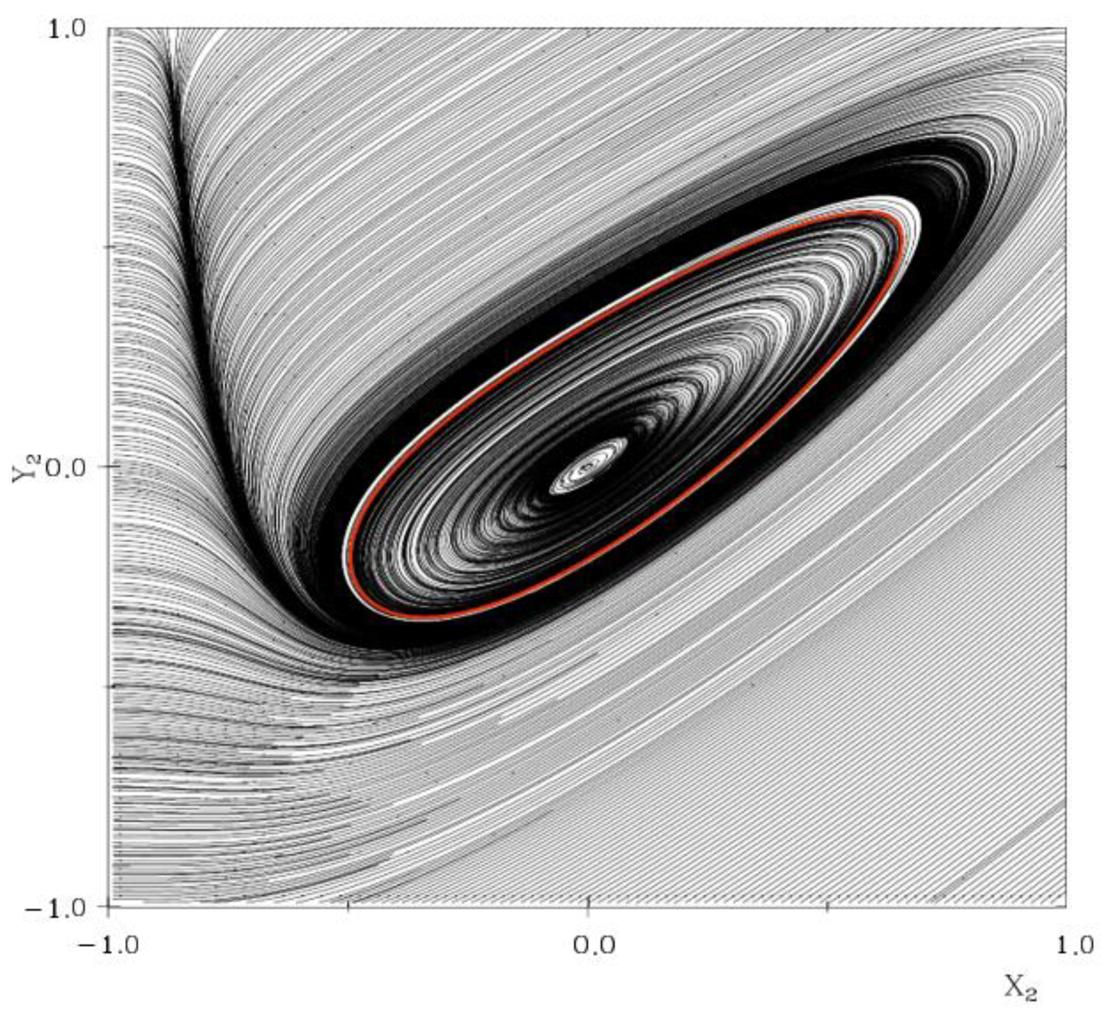
Figure 2.
Time series of three entropy fluxes in the approach of the RCE: (red) the flux of entropy from the sea to air, (blue) the flux of entropy from the air to space due to radiative cooling and (black) the total internal generation of entropy due to mixing and rainwater evaporation.
Figure 2.
Time series of three entropy fluxes in the approach of the RCE: (red) the flux of entropy from the sea to air, (blue) the flux of entropy from the air to space due to radiative cooling and (black) the total internal generation of entropy due to mixing and rainwater evaporation.

Figure 3.
Time series of (left) the horizontally averaged air temperature and (right) the relative humidity near (red) the sea surface and (black) at a 4.5 km altitude. The air surface temperature is displayed with its value minus 26 K.
Figure 3.
Time series of (left) the horizontally averaged air temperature and (right) the relative humidity near (red) the sea surface and (black) at a 4.5 km altitude. The air surface temperature is displayed with its value minus 26 K.
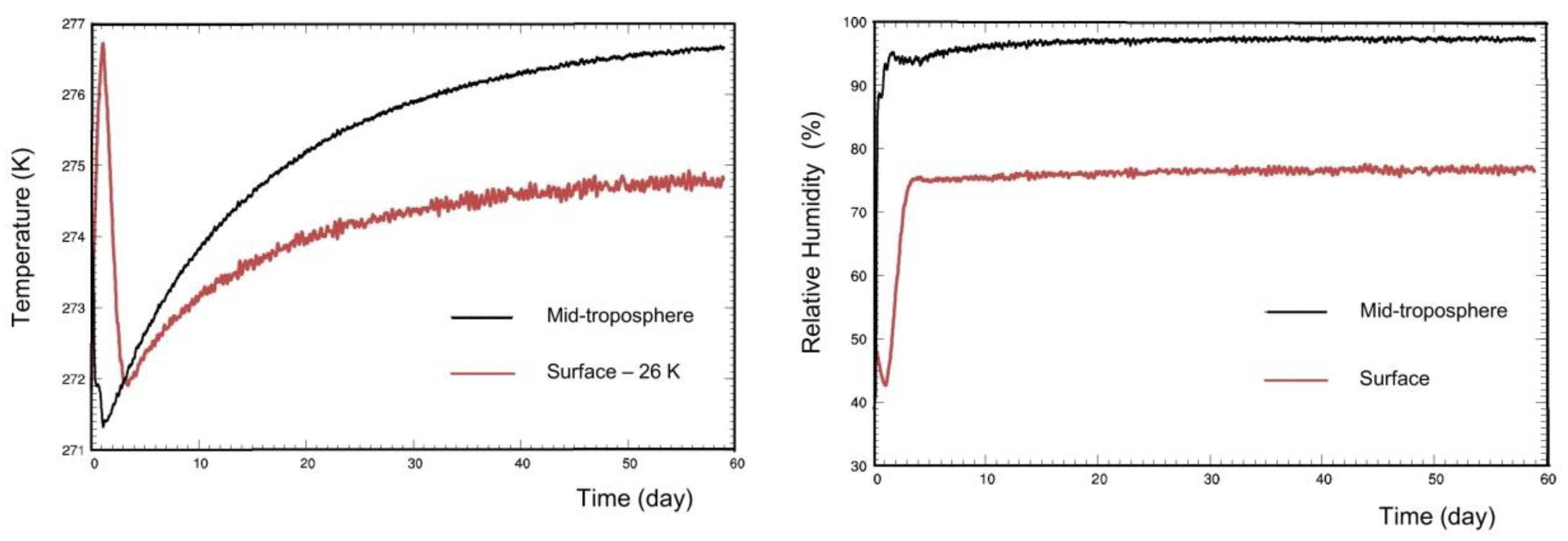
Figure 4.
Long timescale versus the dimensionless number Nw when the radiative cooling rate is 1 °C/day. Symbol □ represents the CRM simulation results; symbol ■ and the dashed line represent the analytic result from Equation (5).
Figure 4.
Long timescale versus the dimensionless number Nw when the radiative cooling rate is 1 °C/day. Symbol □ represents the CRM simulation results; symbol ■ and the dashed line represent the analytic result from Equation (5).

Figure 5.
Amplitude of (left) the air surface temperature and (right) the surface energy flux against the forcing period of the surface wind 2π/ω, where the energy flux takes the unit of the equivalent water evaporation. The circles denote the CRM results, and the solid lines denote the analytic results of Equation (8). The dashed lines over small period denote the active mode where the difference between the sea surface entropy and the air surface entropy is fixed; the dashed lines over long periods signify the passive mode where the surface entropy flux is fixed.

Figure 6.
Same as Figure 5 except against the forcing period of the radiative cooling. The dashed lines over the small period denote the active mode where the top entropy flux has no effect on the surface entropy flux; the dashed lines over the long period denote the passive mode where the top entropy flux controls the surface entropy flux via convective clouds.

Figure 7.
Diagrammatical analysis of the buoyancy of an air parcel that ascends adiabatically from the surface. The blue and red solid lines represent the vertical profiles of the mean moist entropy and the saturation moist entropy in the tropics, respectively. If a surface air parcel ascends adiabatically, its moist entropy and saturation moist entropy follow the black dashed line and the green dashed line, respectively, from the surface level A/B to the lifted condensation level C, the level of free convection D and finally to the cloud top E. Its buoyancy is directly proportional to the difference in entropy between the green line B–C–E and the red line.

Figure 8.
Vertical cross sections of (top) the radar reflectivity and (bottom) the Doppler velocity of an MCS observed on 31 July 2007 over the Pacific Ocean south of Costa Rica during the TC4 experiment along two EDOP flight tracks. In the bottom panes, red (or positive) and blue (or negative) represent the downward and upward motions, respectively; the white areas surrounded by the red ones indicate the Doppler folding (or the Doppler velocity larger than 34 m s−1). (Left) The flight track over 1549–1605 UTC is parallel to the leading edge of the MCS, and (right) the track over 1634–1640 UTC is perpendicular to the leading edge of the MCS and right across the center of the MCS.

Figure 9.
Horizontal distribution of the cloud–ice mixing ratio at 8.6 km (left; representing cloud anvil) and the graupel mixing ratio at 5 km (right; representing convective cores) at 0400 UTC 11 August 2006. The results come from the two numerical experiments with a (top) high and (bottom) low number concentration of activated IN. The broad anvil in the experiment with the plentiful activated IN (top/left) agrees with the in-situ satellite and radar observations during the field campaign of the AMMA (the African Monsoon Multidisciplinary Analysis) over West Africa. Adapted with permission from Zeng et al. (2013) [43].

Figure 10.
Schematic showing (green area) the deep and shallow convective clouds in two adjacent columns are connected by (golden line) a large-scale vertical circulation. The two columns maintain the WTG in the mid-troposphere, and each column is characterized with the three layers of (blue) the UT, (red) PBL and (gray area) sea surface.

Figure 11.
Time series of (green) the dimensionless surface entropy X, (red) the UT entropy Y and (blue line) the UT cloud fraction Z in the system of Equations (18)–(20) (see Appendix A for the definitions and parameters used). The horizontal axis of time is scaled with = 28 days (or ~ 1 month) as the unit.

Figure 12.
Modeled time series of (left) the surface moist entropy and (right) the entropy flux from the sea to the air in the (red) test and (blue line) reference columns.
Figure 12.
Modeled time series of (left) the surface moist entropy and (right) the entropy flux from the sea to the air in the (red) test and (blue line) reference columns.

Figure 13.
Modeled time series of (left) the horizontally averaged surface wind speed and (right) the entropy flux at z = 0.75 km in the (red) test and (blue line) reference columns.
Figure 13.
Modeled time series of (left) the horizontally averaged surface wind speed and (right) the entropy flux at z = 0.75 km in the (red) test and (blue line) reference columns.

Figure 14.
Vertical profiles of the moist entropy (blue line) and the saturation moist entropy (red line) obtained from the dropsonde at ~1551 UTC on 31 July 2007 during the TC4 experiment. The dropsonde was released from the DC-8 aircraft flying at an altitude of 12 km to measure the atmospheric temperature, pressure, wind and relative humidity near the MCS shown in Figure 8.

Figure 15.
Time series of (green) X2 the dimensionless surface entropy in the test column and (red) Y2 the saturation moist entropy at z = 2 km in the reference column in the system of Equation (22) and Equation (24) (see Appendix C for the definitions and parameters used). The horizontal axis of time is scaled with = 28 days as the unit.

Figure 16.
Time series of (green) the dimensionless air surface entropy X, (red) the UT entropy Y, (blue) the UT cloud fraction Z and (black) the sea surface entropy Ψ in the system of Equations (28), (29), (19) and (20) (see Appendix B for the definitions and parameters used). The horizontal axis of time is scaled with = 28 days (or ~1 month) as the unit.

Disclaimer/Publisher’s Note: The statements, opinions and data contained in all publications are solely those of the individual author(s) and contributor(s) and not of MDPI and/or the editor(s). MDPI and/or the editor(s) disclaim responsibility for any injury to people or property resulting from any ideas, methods, instructions or products referred to in the content. |
© 2023 by the author. Licensee MDPI, Basel, Switzerland. This article is an open access article distributed under the terms and conditions of the Creative Commons Attribution (CC BY) license (https://creativecommons.org/licenses/by/4.0/).
Share and Cite
MDPI and ACS Style
Zeng, X. Atmospheric Instability and Its Associated Oscillations in the Tropics. Atmosphere 2023, 14, 433. https://doi.org/10.3390/atmos14030433
AMA Style
Zeng X. Atmospheric Instability and Its Associated Oscillations in the Tropics. Atmosphere. 2023; 14(3):433. https://doi.org/10.3390/atmos14030433
Chicago/Turabian StyleZeng, Xiping. 2023. "Atmospheric Instability and Its Associated Oscillations in the Tropics" Atmosphere 14, no. 3: 433. https://doi.org/10.3390/atmos14030433
Note that from the first issue of 2016, this journal uses article numbers instead of page numbers. See further details here.