Characteristic Features of the Antarctic Surface Air Temperature with Different Reanalyses and In Situ Observations and Their Uncertainties

Abstract

Antarctic surface air temperature (SAT) variability is characterized by strong seasonality and regionality, which are associated with the tropical–polar teleconnections and the radiative forcing caused by the concentration changes in ozone and other greenhouse gases. Nevertheless, the sparse in situ observations and the strong disagreement between different reanalysis datasets hinder coherent conclusions about Antarctic SAT variability. In this study, we use a newly developed statistical method, combined maximum covariance analysis (CMCA), to retrieve coherent SAT modes from six reanalysis datasets and 26 station observations. The results show that the Antarctic SAT variability may be dominated by a continental-wide warming/cooling mode, an East–West Antarctic seesaw mode, and a dipole SAT mode around West Antarctica. These SAT modes are strongly associated with three principal modes of Antarctic atmospheric circulation. Furthermore, all six reanalyses can represent these SAT modes well, compared with the observations, despite a clear deviation over the Antarctic Peninsula associated with the biases in the Foehn wind, which may not be clearly reproduced in a low-resolution reanalysis. This study provides an effective means by which to extract coherent signals from all reanalyses and observations to represent the Antarctic SAT variability, and to improve its predictability and projection.

1. Introduction

In recent decades, the Antarctic surface air temperature (SAT) has experienced rapid changes, characterized by strong seasonality and regionality [1,2,3,4,5]. The Antarctic SAT variability typically shows a zonally asymmetric pattern, caused by the opposite SAT anomalies between East and West Antarctica [1,6]. In addition, a series of local features have been observed, including a fast warming of the South Pole since the 1990s [2,7], the absence of Antarctic Peninsula warming in the 21st century [5], and a series of extreme warm events over the Antarctic Peninsula and East Antarctica [8,9]. These features further increase the complexity of the Antarctic SAT variability at different timescales. Characterizing these spatial and temporal features requires precise, high-resolution measurements around the South Pole region, which are unfortunately absent in the present observational system.

Investigations of the Antarctic SAT variability depend on the availability of high-quality in situ observations measured by the Antarctic stations [4,10]. However, these in situ observations are too sparse to provide a complete representation of the entire Antarctic [4]. As a complement to and proxy of these in situ observations, high-resolution gridded reanalysis datasets play important roles in describing the SAT and circulation variabilities over the entire Antarctic [11,12,13]. However, non-negligible biases occur in all the reanalysis datasets over the Antarctic region [11,13,14], partly due to the low quality of the satellite observations around this area [15], which result in large uncertainties in the reanalyses and deprive us of solid conclusions regarding many key features of the Antarctic [16]. These disadvantages of the in situ observations and reanalyses mean that comparing, validating, and synthesizing all useful datasets over the South Pole region to achieve solid conclusions about the Antarctic SAT variability remain key issues.

The Antarctic SAT variability is affected by many factors, including radiative forcing by greenhouse gases [17] and cloud feedback [18], anomalous atmospheric advection [3,19,20], ocean–sea–ice–atmosphere interactions [21,22], etc. Among these factors, the anomalous atmospheric circulation plays an important role in forming the large-scale patterns of the Antarctic SAT. Several atmospheric circulation patterns have been identified around Antarctica. The most important are the Southern Annular Mode (SAM) and the two Pacific Southern America modes (PSA1 and PSA2). Different metrics have been used to define these large-scale circulation patterns, with the most popular one being the first three principal components of the 500 hPa geopotential height (GPH500) [16]. These circulation modes are strongly associated with the radiative forcing driven by the increase in greenhouse gas and ozone loss [17,23,24], and have been linked to the tropical ocean temperature variability through atmospheric teleconnections [19,20,25,26,27].

These representative circulation modes largely modulate the SAT variabilities through thermal advection and its induced atmosphere–ice–ocean interactions [3,10,19,25,26,28,29]. Previous studies showed that the warming of the northeast Antarctic Peninsula and cooling over the Antarctic continent is usually associated with a positive SAM phase [10,23,28], while the “Antarctic Dipole” (ADP) pattern, referred to as the out-of-phase relationship between the ice and temperature anomalies in the central/eastern Pacific and Atlantic sectors of the Antarctic [30], is closely related to the PSA1 mode [3,29]. More recent studies demonstrated that the seesaw SAT pattern observed between West Antarctica and East Antarctica is partially driven by the PSA2 mode [31]. The linkages between atmospheric circulation modes and SAT variabilities imply the existence of large-scale SAT modes over Antarctica. Nevertheless, the sparse distribution of the in situ observations and the large disagreements between different reanalyses [6,10,11] prevent us from retrieving a robust SAT mode over the entire Antarctic region.

Therefore, a question arises regarding whether it is possible to synthesize all in situ and reanalysis datasets to achieve coherency when retrieving representative SAT modes over the Antarctic. A recently developed spatial–temporal decomposition method, the combined maximum covariance analysis (CMCA, see Methods) method, is a good candidate for performing this multi-dataset decomposition. The CMCA method extracts the strongest coherent patterns from multiple measurements of the same variable by retrieving the primary spatial–temporal modes with the largest covariance among the different datasets [32]. This method offers the possibility of retrieving the most coherent and representative modes of the Antarctic SAT variability from different observational and reanalysis datasets, which are usually strongly associated with detailed physical processes, particularly the anomalous atmospheric circulation pattern and its induced thermal advection. It also provides an opportunity to compare and evaluate different datasets based on the main features of the atmospheric SAT and circulation patterns, which is especially useful, considering the large disagreement between different reanalysis datasets covering the Antarctic region.

In this study, we applied the CMCA method to six reanalysis datasets and 26 station observations. In this way, we retrieved the three most representative SAT patterns with strong agreement among all observations and reanalysis datasets. These SAT patterns are closely linked to the major atmospheric circulation modes according to both statistical analyses and the diagnostics of physical processes. We also compared the characteristics of these SAT modes, using different reanalysis datasets and observations to evaluate the different reanalysis datasets’ ability to capture the mean features of SAT variabilities over Antarctica. Section 2 introduces the datasets and statistical methods used in this study. Section 3 describes the analysis results, with Section 3.1 showing the three leading CMCA modes of the Antarctic SAT and their relationship with SAM and PSA, and Section 3.2 evaluating the diversity among the different datasets and the reanalysis datasets’ ability to capture the main feature of these modes. The seasonality of these SAT modes and their dynamics are discussed in Section 3.3. Section 3.4 discusses the underestimation of the temperature gradient between the east and west coast of the Antarctic Peninsula. The conclusion and discussion are presented in Section 4.

2. Data and Methods

2.1. Data

In this study, we used monthly SAT, GPH500, and zonal (u) and meridional (v) components of the 10 m wind from six reanalysis datasets: (1) the Climate Forecast System Reanalysis (CFSR) [33] from 1979 to 2010 and the NCEP coupled forecast system model version 2 (CFSv2) [34] from 2011 to 2020; (2) the Modern-Era Retrospective Analysis for Research and Applications (MERRA) [35] from 1979 to Feb. 2016; (3) the Modern-Era Retrospective Analysis for Research and Applications, version 2 (MERRA2) [36] from 1980 to 2020; (4) the Japanese 55-year Reanalysis (JRA55) [37]; (5) the Interim reanalysis data from the European Centre for Medium-Range Weather Forecasts (ERA-Interim) [38] from 1979 to Aug. 2019; and (6) the European Centre for Medium-Range Weather Forecasts Reanalysis version 5 (ERA5) [39]. We further calculated the ensemble mean of all six datasets (referred as EnMean). The SATs in all these datasets were interpolated into a 2° × 2° grid before CMCA analysis, while the spatial resolution was 1° × 1° for other variables.

The monthly SAT data observed from 26 Antarctic stations (

Table 1. Stations used in this study.

Number	Name	Latitude	Longitude	Elevation (m)	Period
1	Amundsen–Scott	−90	0	2835	1979–2020
2	Belgrano II	−77.9	325.4	256	1980–2001, 2005, 2007, 2009–2020
3	Bellingshausen	−62.2	301.1	16	1979–2020
4	Byrd	−80	240	1515	1979–2020
5	Casey	−66.3	110.5	42	1979–2020
6	Davis	−68.6	78	13	1979–2020
7	Dumont D’Urville	−66.7	140	43	1979–2020
8	Esperanza	−63.4	303	13	1979–2020
9	Faraday Vernadsky	−65.4	295.6	11	1979–2020
10	Halley	−75.5	333.6	30	1979–2020
11	Marambio	−64.2	303.3	198	1979–2020
12	Mario Zucchelli	−74.7	164.1	92	1988–2005, 2008–2019
13	Marsh	−62.2	301.1	10	1979–2020
14	Mawson	−67.6	62.9	16	1979–2020
15	McMurdo	−77.9	166.7	24	1979–2020
16	Mirny	−66.5	93	30	1979–2020
17	Neumayer	−70.7	351.6	50	1982–2020
18	Novolazarevskaya	−70.8	11.8	119	1979–2020
19	O’Higgins	−63.3	302.1	10	1979–2020
20	Orcadas	−60.7	315.3	6	1979–2002,2004–2020
21	Palmer	−64.3	296	8	1981–2020
22	Rothera	−67.5	291.9	32	1979–2020
23	San Martin	−68.1	292.9	4	1979–2002, 2005–2020
24	Scott Base	−77.9	166.7	16	1979–2018
25	Syowa	−69	39.6	21	1979–2020
26	Vostok	−78.5	106.9	3490	1979–1995, 1997–2020

) were used in this study. These station observations were collected by the Scientific Committee on Antarctic Research (SCAR) Reference Antarctic Data for Environmental Research (READER) database [40]. In addition, monthly SAT observation data for the Byrd station were obtained from the temperature reconstruction performed by the Ohio State University [1].

2.2. The CMCA Method

The CMCA method [32] is an extension of the maximum covariance analysis (MCA). Compared with the MCA, the CMCA method is a useful tool to extract the most coherent information from multiple datasets with the same variable (SAT in this study). Given the non-negligible SAT biases in all reanalysis datasets (Figure 1) and the sparse distribution of the in situ observations over the Antarctic, the CMCA method provides an effective way to extract reliable information from reanalysis and in situ observations about the Antarctic SAT. In this study, CMCA decomposed a covariance matrix between observational datasets and multiple reanalysis datasets of the same variable (SAT).

The SAT anomaly at the 26 stations forms the state variable of the observations ($X_{obs}$), which is a $p\times n$ matrix, with $p$ representing the number of stations (26 in this study) and $n$ denoting the time range of each dataset (monthly data from 1979 to 2020) and serving as the sample size in this analysis. Similarly, the state variable of the SAT anomaly in each reanalysis dataset is a $q\times n$ matrix ($X_{CFSR}$, etc.), where q is the total number of grids in each reanalysis. The matrices of the six reanalyses are further combined into a matrix with the dimensions of $6q\times n$ to form the state variable of all six reanlayses, provided they represent the same variable and share the same unit:

$$X_{rea}=\left[\begin{array}{c}{X}_{CFSR}\\ X_{MERRA}\\ X_{MERRA2}\\ X_{JRA55}\\ X_{ERA-In}\\ X_{ERA5}\end{array}\right]$$

(1)

The covariance matrix $C$ is calculated as follows

$$C=\frac{1}{n-1}{X}_{rea}{X}_{obs}^T$$

(2)

where $n$ is the sample size of these datasets.

We then performed singular-value decomposition (SVD) on the covariance matrix $C$ to retrieve the largest coherent modes in these datasets by maximizing their cross-covariance.

$$C=US{V}^T$$

(3)

The matrices $U$ and $V$ are singular vectors of the covariance matrix $C$ and represent the spatial patterns of each SVD mode of the reanalyses and observation, respectively. $S$ contains the singular values that represent the covariance explained by each mode. $U$ is a combined matrix containing the spatial patterns of the six reanalyses, with the same structure as the state variable $X_{rea}$:

$$U_{rea}=\left[\begin{array}{c}{U}_{CFSR}\\ U_{MERRA}\\ U_{MERRA2}\\ U_{JRA55}\\ U_{ERA-In}\\ U_{ERA5}\end{array}\right]$$

(4)

We removed the linear trend in each observational and reanalysis dataset before the CMCA. For the detailed method, please refer to Li, Carlson, and Lacis [32].

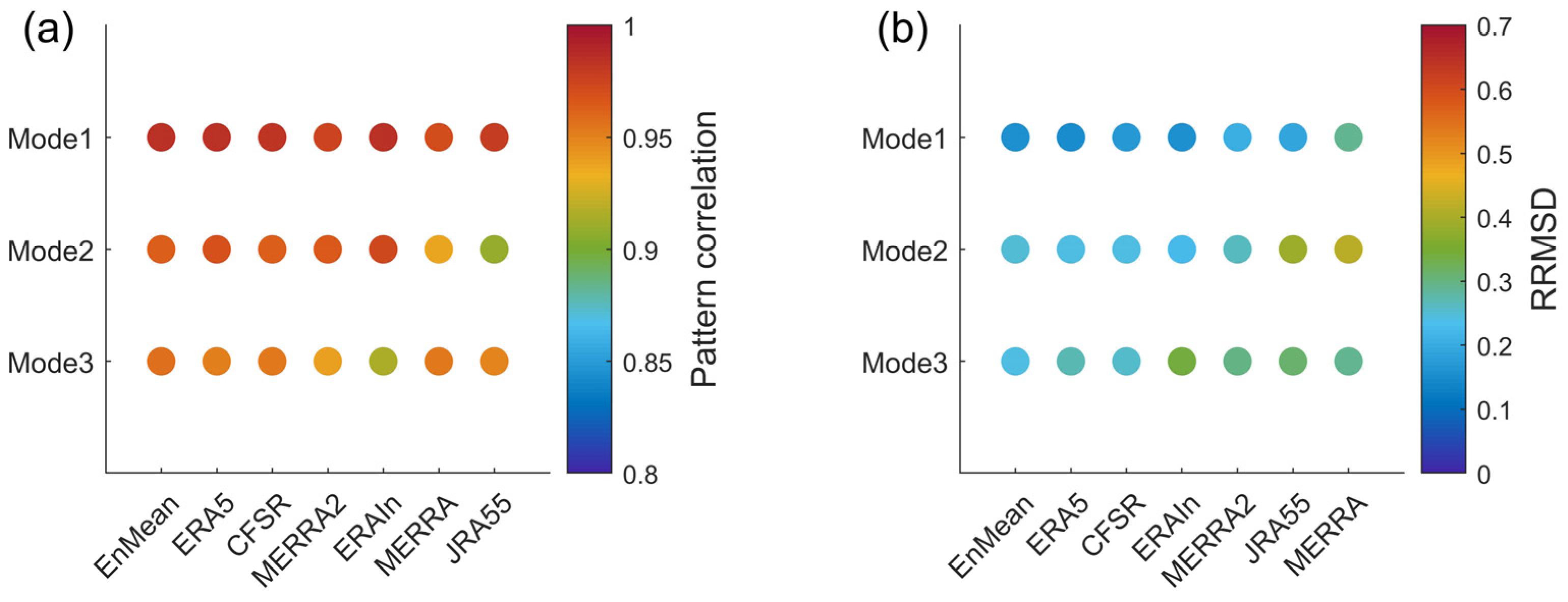
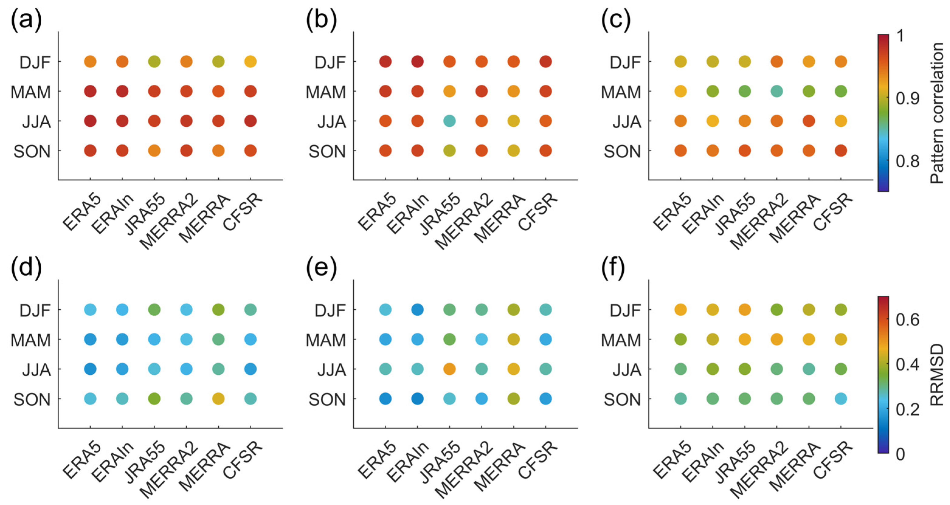
2.3. Spatial Pattern Correlation

To evaluate the consistency of the spatial patterns between reanalyses and observations in each CMCA mode, we calculated the area-weighted correlation coefficients between the spatial patterns of the observations and the reanalyses. Notably, we interpolated the SAT of each reanalysis dataset onto the position of the station observations before calculating the spatial pattern correlation, to allow comparison between different datasets.

2.4. Ratio of Root Mean Square Deviation

To evaluate the consistency between the spatial patterns of the reanalyses and observations in each mode, we calculated the ratio of the root mean square deviation (RRMSD) of these spatial patterns. The RRMSD is defined as

$$RRMSD=\frac{RMSD}{std}$$

(5)

Here, $RMSD$ represents the root mean square deviation of the spatial pattern between reanalyses and observations, and $std$ is the standard deviation of the spatial pattern in the observation.

2.5. The PCA Method

In this study, the SAM, PSA1, and PSA2 modes were defined as the first three principal components retrieved from the monthly GPH500 anomaly of ERA5 using the Principal Component Analysis (PCA), following the definition of Mo [16]. Notably, the results were similar no matter whether we use rotated PCA or PCA without rotation. However, the SAM, PSA1 and PSA2 mode is usually defined as the leading modes of GPH500 using the unrotated PCA method [16,41,42]. Therefore, we also used the PCA without rotation in this work.

2.6. Correlation and Regression

The Pearson correlation coefficients between the time series of CMCA modes and the SAM, PSA1, and PSA2 were calculated to investigate the relationship between the SAT modes and the atmospheric circulation modes. We regressed the SAT, GPH500, and u, v components of the 10 m wind of the reanalyses against the time series of the first three CMCA modes to clarify the dynamics underlying these statistical modes. Student’s t-test was applied to calculate the significance level of the correlation and regression coefficients.

3. Results

3.1. Coherent SAT Modes in the Reanalyses and In Situ Observations

We first calculated the CMCA modes in all reanalyses and observations using monthly SAT data. The first three CMCA modes (Figure 2) explain more than 90% of the total covariance, representing the majority of the interannual and decadal variabilities in Antarctica.

The first mode (Figure 2a) shows a continental warm (cold) anomaly over the entire Antarctic (hereafter referred to as Antarctic continental mode), with a spot of cold (warm) signal around the north end of the Antarctic Peninsula. The second mode (Figure 2b) shows a seesaw-like SAT pattern, with opposite temperature anomalies between East and West Antarctica (hereafter referred to as the Antarctic seesaw mode). The anomalous temperature patterns of the third mode (Figure 2c) are concentrated around western Antarctica, with opposite SAT anomalies between the Antarctic Peninsula–West Antarctica and the Ross sea area, representing the well-known Antarctic dipole mode [30,43].

We further evaluated the reanalyses by comparing the ensemble mean of the CMCA modes of all six reanalysis datasets with the observations. Each CMCA mode in the reanalyses was first interpolated to the locations of the in situ observations, and the deviation between the reanalyses and the observations of the first three CMCA modes are illustrated in Figure 2d–f. The results show negligible differences between the reanalysis modes and the observation. This consistency indicates that the ensemble mean of the reanalysis modes can capture the main features of the observed SAT variabilities and these isolated SAT observations could apply to the entire Antarctic continent (Figure 2a–c).

We further retrieved the atmospheric circulation patterns associated with the above Antarctic SAT modes by regressing the GPH500 against the time series of the first three CMCA modes (Figure 3a–c). We then compared them with the classic atmospheric circulation patterns over the southern hemisphere, namely the SAM (Figure 3d), and the first (Figure 3f) and second (Figure 3e) PSA modes (see Method). The circulation patterns associated with the first three SAT modes showed strong coherency with these classic atmospheric circulation patterns (Figure 3).

The Antarctic continental mode (Figure 2a) is associated with an anomalous high-pressure (low-pressure in negative phase) center over the entire Antarctic continent (Figure 3a), resembling the (negative phase of) SAM (Figure 3d), with a spatial pattern correlation of 0.97. The circulation patterns (Figure 3b,c) associated with the Antarctic seesaw (the second CMCA, Figure 2b) and the Antarctic dipole (the third CMCA, Figure 2b) modes are characterized by two Rossby wave trains, both with high–low–high-pressure centers over the Pacific sector of the Southern Ocean, despite a phase shift occurring between these two wave trains. These circulation modes are very similar to the PSA2 (Figure 3e) and PSA1 (Figure 3f) patterns, with spatial pattern correlations over the Pacific sector of 0.8 and 0.91, respectively. Remarkably, the time series of the first three SAT modes are also highly correlated with those of the SAM, PSA2, and PSA1, with correlation coefficients of 0.80, 0.55, and 0.62, respectively (

Table 2. The correlation coefficients between the time series of the first three modes of the combined maximum covariance analysis (CMCA) for annual surface air temperature (SAT) anomalies, and of the three principal components of the circulation over the Antarctic: the southern annular mode, and the first and second Pacific South American modes.

	SAM	PSA1	PSA2
Mode1 (58.0%)	0.80	0.19	−0.16
Mode2 (24.5%)	−0.02	0.20	0.55
Mode3 (7.8%)	−0.25	0.62	−0.07

).

These coherencies between surface temperature and atmospheric circulation modes indicate that the patterns retrieved by CMCA in this study are beyond the statistical analysis results, but represent strong physical links between these SAT patterns and the leading modes of the southern-hemispheric atmospheric circulation variability. The poleward (equatorward) shift in the jet system associated with SAM anomalies (Figure 3d) may help explain the continental-wide (Figure 2a) anomalous SAT pattern in the CMCA Mode1, whereas the warm and cold advections induced by the high–low pressure centers of PSA2 (Figure 3e), and the thermal advections associated with the anomalous Amundsen Sea Low (ASL, Figure 3f), contribute to the zonally asymmetric Antarctic seesaw (Figure 2b) and dipole (Figure 2c) patterns, respectively.

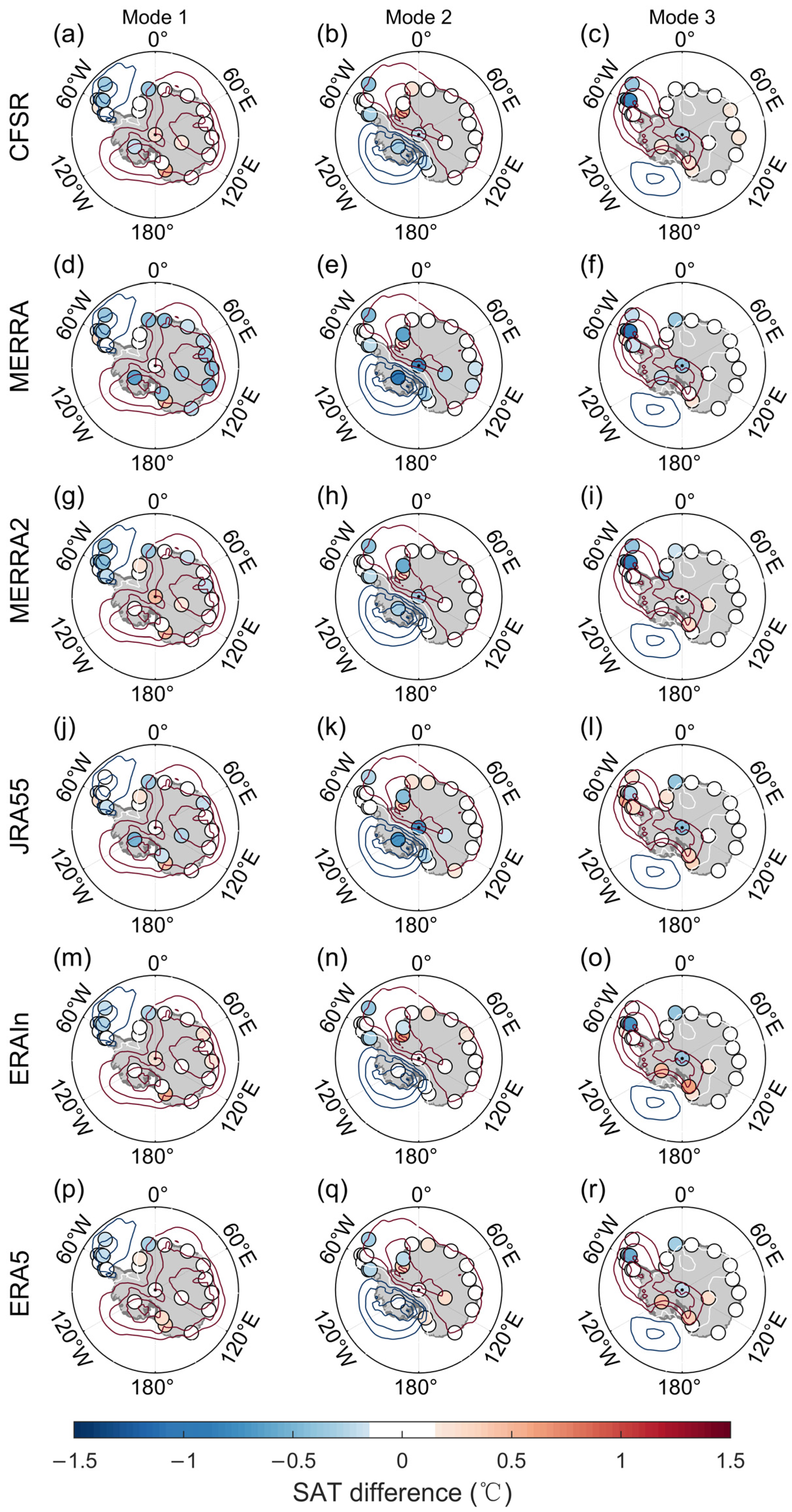
3.2. Diversity of Different Reanalyses According to the Leading CMCA Modes

The similarity between the ensemble mean CMCA modes of the six reanalyses and those of the observations (Figure 2) implies coherency between the observations and reanalyses of the main SAT features. We further evaluated this coherency among different reanalysis datasets by intercomparing the spatial patterns in these modes in each of the six reanalyses (Figure 4). The results show a strong similarity among all six datasets, with mode one in all six datasets representing the continental warming/cooling pattern (Figure 4a,d,g,j,m,p), and modes two and three all represent the Antarctic seesaw (Figure 4b,e,h,k,n,q) and Antarctic dipole (Figure 4c,f,i,l,o,r) patterns, respectively. The spatial patterns of these SAT modes are almost identical among all six datasets, with minor differences appearing in the amplitude of local signals.

To further quantify the similarities in the spatial patterns of these CMCA modes between different reanalyses, we calculated the spatial pattern correlation between the CMCA mode of each reanalysis and that of the observations (Figure 5a). All reanalysis patterns were highly correlated with those of the observations. The correlation coefficients of Mode1 are all above 0.97 (Figure 5a), with the correlation coefficients of Mode2 and Mode3 typically being higher than 0.95. The correlations for the JRA55 in Mode2 and ERA-Interim in Mode3 were relatively lower, but still above 0.9. Therefore, the first three CMCA modes show strong coherency not only between observations and reanalyses, but also among different reanalysis datasets. This coherency suggests that the first three CMCA modes successfully retrieve the leading coherent features of the Antarctic SAT variabilities, with strong agreement between all datasets used in this study.

We further highlighted the deviation of these CMCA modes in each reanalysis dataset by calculating the difference between these reanalysis modes and those of the observations at the 26 Antarctic stations (Figure 6), with the left, middle, and right columns showing the deviations of the six reanalyses in Mode1, Mode2, and Mode3, respectively. In most of the reanalyses, the differences are negligible, although the MERRA and JRA55 in CMCA Mode2 (Figure 6e,k) show relatively strong negative anomalies over central and western Antarctica (Amundsen–Scott and Byrd stations), and several stations over the Peninsular region in CMCA Mode3 show a clear (negative) anomaly in most reanalyses (Figure 6c,f,i,l,o,r).

We further quantified these deviations by calculating the RRMSD between all six reanalyses and the observations of the first three CMCA modes (Figure 5b). Most of the reanalysis modes show a low RRMSD, below 0.25, although the MERRA and JRA55 CMCA Mode2 have a higher RRMSD of about 0.5. The RRMSDs of several reanalyses in Mode3 reached 0.4. All agreed well with the detailed features revealed by Figure 4 and Figure 6.

Previous studies revealed that strong disagreement and diversity exist among the different reanalysis datasets representing the SAT variability over the Antarctic [6,11,14], with large biases found between those reanalyses and in situ observations [11,13,44]. However, our results show a strong coherency among all six reanalyses and the in situ observations when representing the first three CMCA modes. As these CMCA modes capture more than 90% of the covariance among these datasets, our results imply that most of the reanalyses can capture the main spatial and temporal features of the Antarctic SAT variability, especially as these variabilities are strongly associated with the main circulation patterns over the Antarctic region.

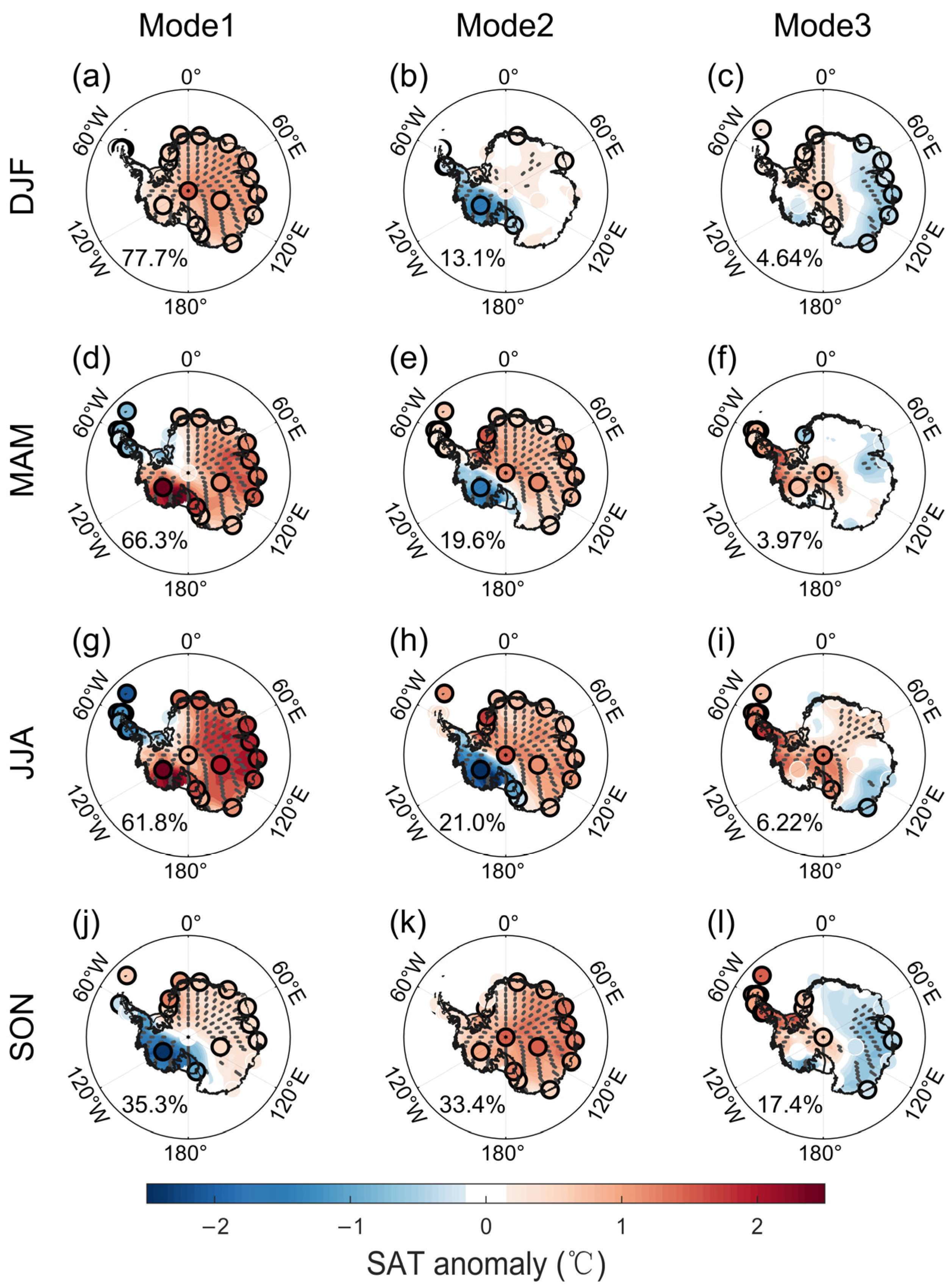
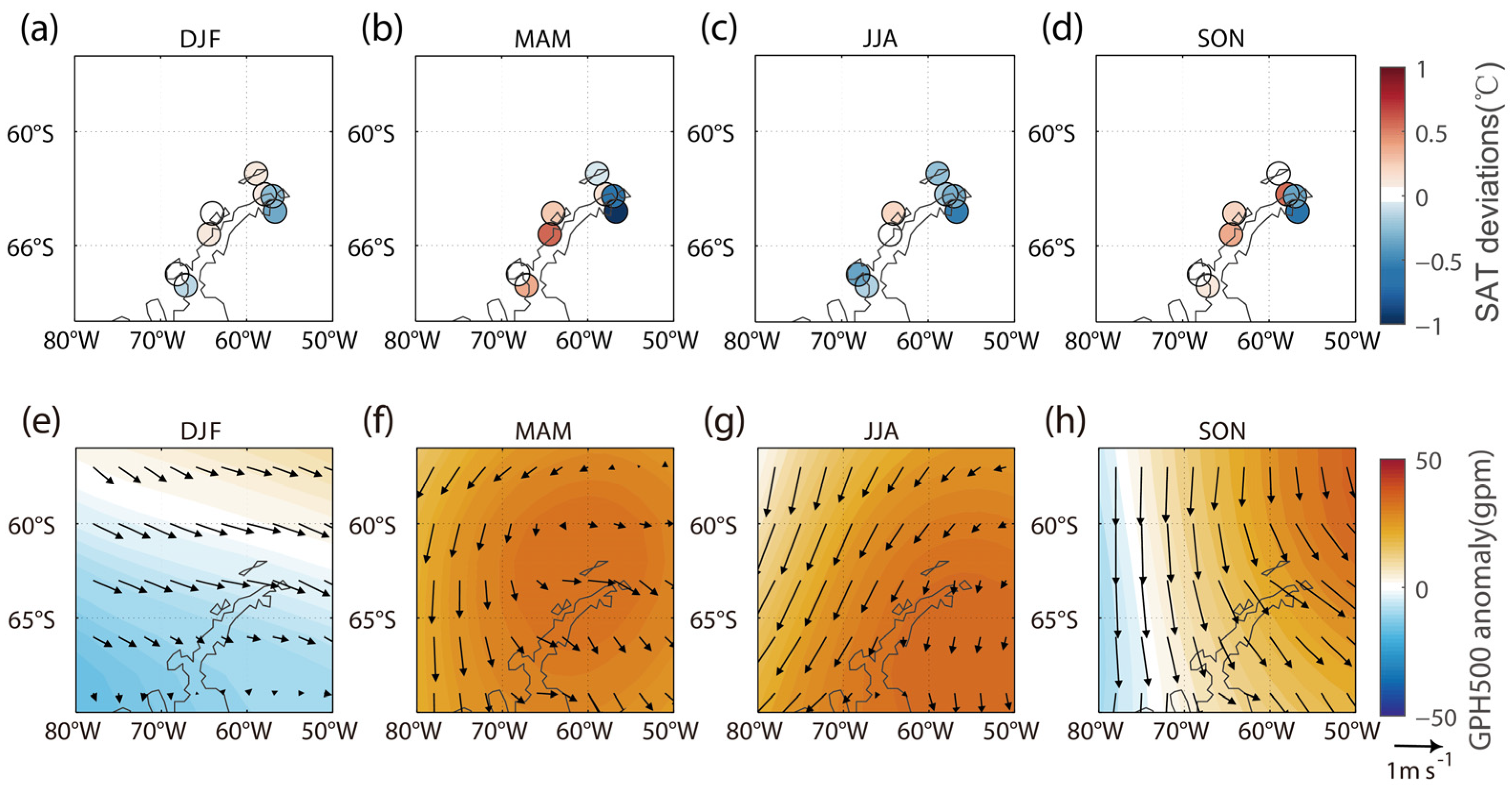
3.3. Seasonality of the CMCA Modes

The SAT variability over the Antarctic shows a strong seasonality. To evaluate the leading modes of the Antarctic SAT for different seasons, we further performed CMCA decomposition among the observations and reanalyses for the four seasons. The spatial patterns of these seasonal CMCA modes are shown in Figure 7, with each row showing the three leading modes for each season. The CMCA modes for different seasons resemble those of the annual decomposition (Figure 2a–c), with the three leading modes representing the Pan-Antarctic continental warming/cooling pattern (Figure 7a,d,g,j for DJF, MAM, JJA, and SON, respectively), the seesaw SAT pattern between Eastern and Western Antarctica (Figure 7b,e,h,k), and the dipole SAT mode around West Antarctica (Figure 7c,f,i,l), respectively. These leading modes explain 95%, 90%, 89%, and 86% of the covariances for each season, respectively, indicating that the majority of the SAT variability is well represented by these CMCA modes.

Nevertheless, the regional features of each mode slightly differ for different seasons. In the CMCA decomposition for austral spring (SON), the order of the first (Figure 7j) and the second (Figure 7k) modes are switched, with the first mode representing the East–West Antarctic seesaw pattern (with the represented covariance of 35.3%) and the second representing the continental warming/cooling pattern (33.4% of covariance). This difference indicates that the thermal advection induced by the PSA2 pattern may contribute more to the Antarctic SAT variability in austral spring (SON). In the continental mode (Figure 7a,k) for austral summer and spring, the continental-wide warming/cooling anomaly is relatively weaker than the other two seasons, with the spot of cooling/warming signal around the Antarctic Peninsula disappearing. In addition, the seesaw and dipole SAT modes (Mode2 and Mode3, Figure 7b,c) for austral summer (DJF) are relatively weaker than those in other seasons, partly due to the weakened Rossby wave dynamics in the summer hemisphere [19,29].

We further quantified the deviations in each CMCA mode for all four seasons by calculating the difference between the reanalysis modes and the observations (Figure 8). The difference in most of the CMCA modes is negligible, with the absolute value of the deviations being less than 0.2 °C in most Antarctic stations. However, for the stations around the Antarctic Peninsula, several CMCA modes showed strong deviations for different seasons (Figure 8c,f,h,i,l). In particular, the deviation over the Antarctic Peninsula in Mode3 was relatively larger than that in the other two modes. The largest difference, reaching −0.96 °C, between the reanalyses and observational modes appeared at the Marambio station for austral autumn (MAM, Figure 8f), which is located on the east coast of the Antarctic Peninsula. Two stations (the Faraday and San Martin stations, Figure 8f) on the west coast of the Peninsula show positive deviations of 0.57 °C and 0.37 °C, respectively.

We further quantified the seasonal coherency between reanalyses and observations by calculating the correlation coefficients between the reanalyses and observational time series of the first three CMCA modes. Most of the coefficients were larger than 0.9, reemphasizing the coherency between the reanalyses modes and those of the observations for all four seasons, although the correlations reduced to 0.85 for summer (DJF), autumn (MAM), and winter (JJA) in Mode3.

The spatial pattern correlation (Figure 9a–c) and the RRMSD (Figure 9d–f) of these reanalysis modes were also examined for all four seasons. For the first two CMCA modes, most reanalysis datasets can capture the observation features for each season, with a pattern correlation usually higher than 0.95, and an RRMSD of less than 0.25. Among the reanalysis datasets, ERA5, ERA-Interim, MERRA2, and CFSR show comparable skills, with a high pattern correlation and low RRMSD, while JRA55 and MERRA show relatively larger differences in the in situ observations for these two modes (Figure 9a,b,d,e). Mode2 of JRA55 for austral winter (JJA, Figure 9b,e) shows relatively larger deviations from station observations according to both pattern correlation (0.85) and RRMSD (0.49). For Mode3, the spatial pattern correlation (Figure 9c) in most of the reanalyses is relatively lower, with the RRMSD being relatively higher (Figure 9f). Most reanalysis patterns for austral autumn (MAM, Figure 9c) show a low correlation, reaching 0.85 for Mode3. Compared with other reanalyses, ERA5 and MERRA2 show relatively high skills for MAM and DJF, respectively. All reanalyses show a similar performance for JJA and SON, with correlations above 0.9 and an RRMSD below 0.4. The low correlations for Mode3 reemphasize that the deviation over the Antarctic Peninsula (Figure 7c,f,i,l) may have a strong influence on the coherency between reanalyses and observations when representing the Antarctic dipole mode.

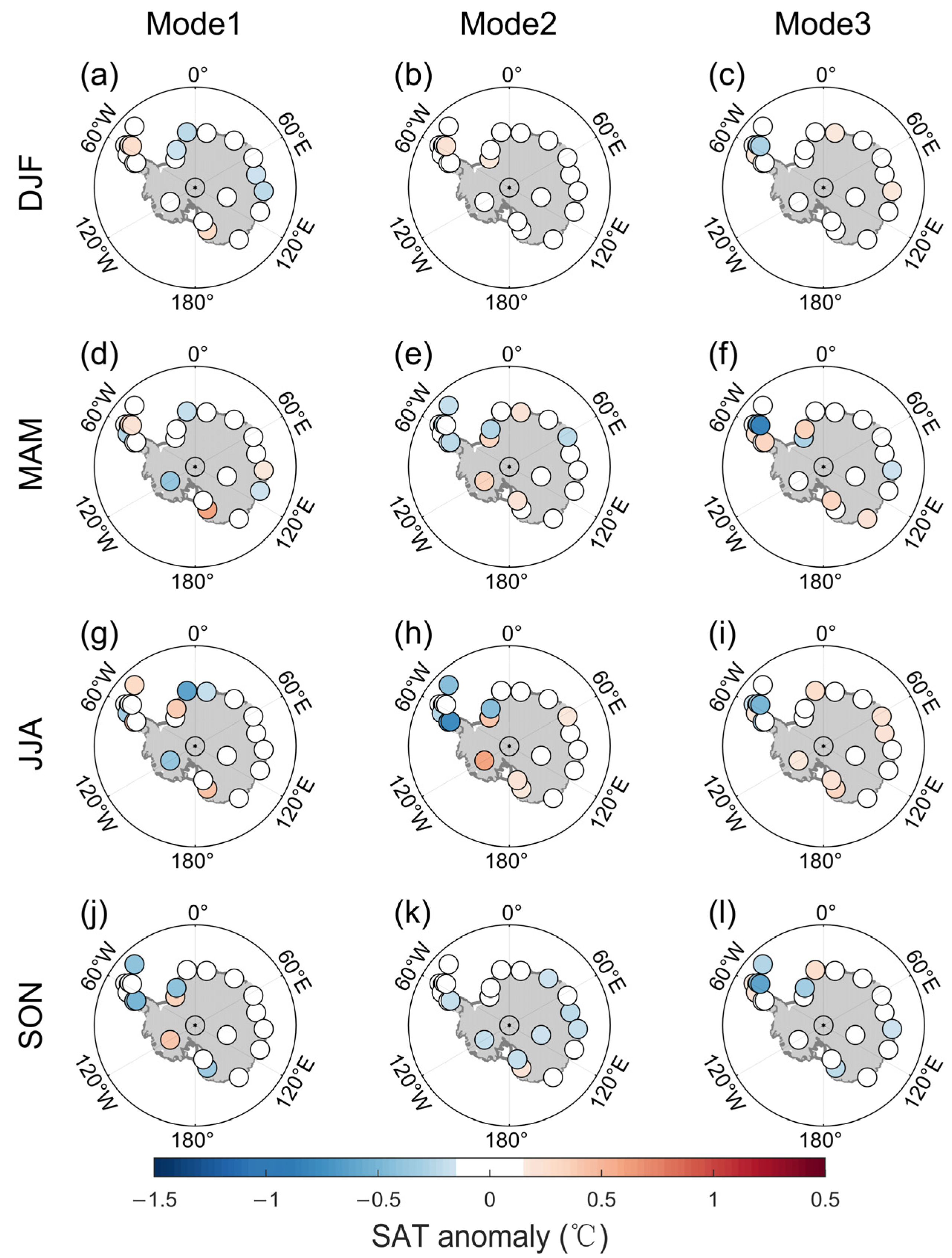
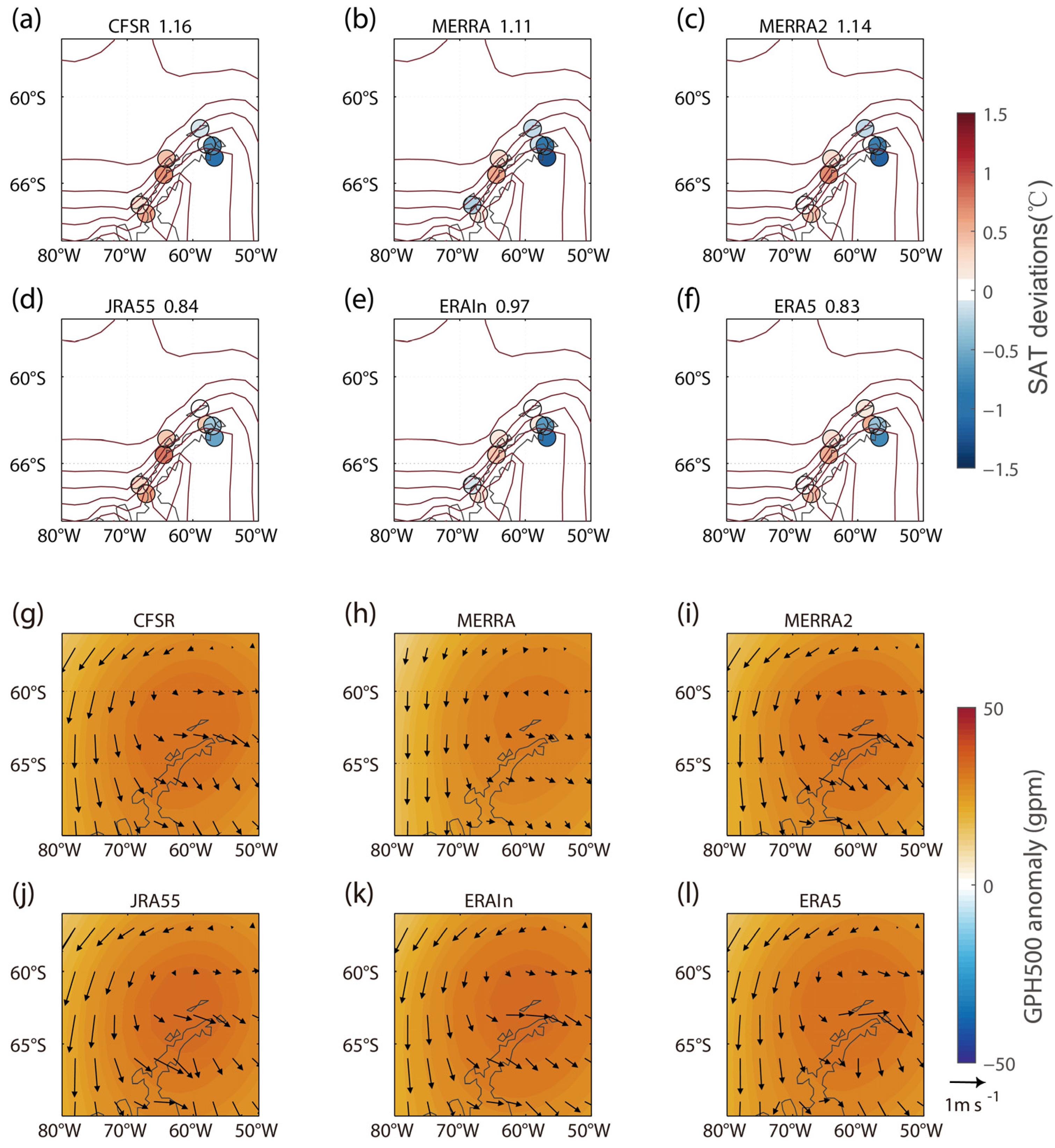
3.4. The Deviation over the Antarctic Peninsula

We further evaluated the difference in Mode3, with a focus on the stations over the Antarctic Peninsula for austral autumn (MAM). As shown in Figure 10 a–f, in all reanalyses, the SAT patterns associated with Mode3 showed a positive deviation over most of the stations on the west coast, but a negative deviation on the east coast. We further illustrated the surface wind pattern associated with Mode3 for all reanalysis datasets (Figure 10g–l). The results show that the SAT pattern over the Peninsula region is tightly associated with an anti-cyclonic circulation pattern, with a surface wind blowing across the Peninsula from the west to the east coast (Figure 10g–l).

Previous studies indicated that the regional temperature variability around the Antarctic Peninsula is highly influenced by the Foehn wind [9,45,46,47]. The Foehn wind is induced by the adiabatic heating at the lee slope of the Trans-Antarctic Mountains, which contributes to the steep topography over the Antarctic Peninsula [45,47]. However, as they are limited by the spatial resolution, most reanalysis datasets cannot resolve this steep topography over the Antarctic Peninsula, and thus may underestimate the effect of the adiabatic wind, leading to an opposite sign for the deviation between the east and west coast (Figure 10a–f).

We further evaluated this opposite sign of SAT deviation between the east and west coast of the Peninsula for other seasons (Figure 11). This deviation is relatively stronger for austral spring (Figure 11d) and autumn (Figure 11b), largely due to the stronger wind anomaly across the Peninsula (Figure 11h,f) for these two seasons.

4. Discussion

In recent decades, the climatic changes over the Antarctic have attracted increasing attention, largely due to their potential impacts on the global sea level rise and the energy balance of the Earth system. The Antarctic SAT variability, at multiple time scales, is characterized by strong seasonality and regionality. However, the sparse in situ observations and the disagreement between multiple reanalysis datasets and observations prevent us from capturing the complexity of the Antarctic SAT variability.

In this study, we aimed to retrieve coherent patterns of multiple observational and reanalysis datasets describing the main features of the Antarctic SAT variability. By adopting a newly developed method, the CMCA decomposition, we retrieved the leading modes of the Antarctic SAT by maximizing the covariance among all these datasets. The first three leading modes captured more than 90% of the total covariance. Mode1 is characterized by a Pan-Antarctic, continental-wide warming/cooling pattern, while Mode2 and Mode3 represent the East–West Antarctic seesaw and the dipole SAT mode around the West Antarctic, respectively. These SAT modes are tightly associated with the circulation anomalies through thermal advection and its related atmosphere–ice–ocean interactions. The continental mode is associated with the SAM, whereas the seesaw and dipole SAT modes are primarily induced by the PSA2 and PSA1 circulation patterns, respectively.

We further evaluated the reanalysis datasets’ ability to reproduce the observed SAT variability according to the retrieved CMCA modes. Although previous studies revealed strong disagreement among different reanalyses, as well as between the reanalyses and in situ observations, our study indicated that the six reanalyses represent the main features of the leading CMCA modes well, compared to the observations.

The spatial and temporal correlation coefficients between the reanalysis and observational modes are almost all higher than 0.9, although limited deviations exist in detailed features between different datasets. In particular, differences between central and western Antarctica exist in the MERRA and JRA55 for the second CMCA mode. In addition, the differences between the reanalyses and the in situ observations for the peninsula region are relatively larger in CMCA Mode3, especially for austral autumn (MAM). This difference is characterized by an opposite deviation between the east and west coast of the Antarctic Peninsula, largely associated with the effect of topography-induced adiabatic wind, which is not very well represented in a low-resolution reanalysis. Despite these differences, the main features of the observed SAT patterns can be reproduced by most of the reanalyses, according to our decomposition results.

The strong coherency between all reanalyses and the in situ observations implies that the CMCA method is an ideal candidate for capturing the broad agreement among different measurements of the same variable; in this study, the variable was the SAT over the Antarctic. In addition, the SAT modes retrieved by this statistical method are shown to be tightly associated with specific physical processes, which may help to more effectively evaluate the evolution of the Antarctic SAT, as well as its physical mechanisms, global impacts, and predictability. This method may also have the potential to achieve broad agreement regarding the SAT trend over the Antarctic among different datasets, which is crucial to the future projection of the Antarctic climate and will be a main focus of our future study.

References

1. Bromwich, D.H.; Nicolas, J.P.; Monaghan, A.J.; Lazzara, M.A.; Keller, L.M.; Weidner, G.A.; Wilson, A.B. Central West Antarctica among the most rapidly warming regions on Earth. Nat. Geosci. 2013, 6, 139–145. [Google Scholar] [CrossRef] [Green Version]
2. Clem, K.R.; Fogt, R.L.; Turner, J.; Lintner, B.R.; Marshall, G.J.; Miller, J.R.; Renwick, J.A. Record warming at the South Pole during the past three decades. Nat. Clim. Chang. 2020, 10, 762–770. [Google Scholar] [CrossRef]
3. Ding, Q.; Steig, E.J.; Battisti, D.S.; Küttel, M. Winter warming in West Antarctica caused by central tropical Pacific warming. Nat. Geosci. 2011, 4, 398–403. [Google Scholar] [CrossRef] [Green Version]
4. Turner, J.; Colwell, S.R.; Marshall, G.J.; Lachlan-Cope, T.A.; Carleton, A.M.; Jones, P.D.; Lagun, V.; Reid, P.A.; Iagovkina, S. Antarctic climate change during the last 50 years. Int. J. Climatol. 2005, 25, 279–294. [Google Scholar] [CrossRef]
5. Turner, J.; Lu, H.; White, I.; King, J.C.; Phillips, T.; Hosking, J.S.; Bracegirdle, T.J.; Marshall, G.J.; Mulvaney, R.; Deb, P. Absence of 21st century warming on Antarctic Peninsula consistent with natural variability. Nature 2016, 535, 411–415. [Google Scholar] [CrossRef] [Green Version]
6. Nicolas, J.P.; Bromwich, D.H. New reconstruction of Antarctic near-surface temperatures: Multidecadal trends and reliability of global reanalyses. J. Clim. 2014, 27, 8070–8093. [Google Scholar] [CrossRef]
7. Stammerjohn, S.E.; Scambos, T.A. Warming reaches the South pole. Nat. Clim. Chang. 2020, 10, 710–711. [Google Scholar] [CrossRef]
8. King, J.C.; Bannister, D.; Hosking, J.S.; Colwell, S.R. Causes of the Antarctic region record high temperature at Signy Island, 30th January 1982. Atmos. Sci. Lett. 2017, 18, 491–496. [Google Scholar] [CrossRef] [Green Version]
9. Xu, M.; Yu, L.; Liang, K.; Vihma, T.; Bozkurt, D.; Hu, X.; Yang, Q. Dominant role of vertical air flows in the unprecedented warming on the Antarctic Peninsula in February 2020. Commun. Earth Environ. 2021, 2, 133. [Google Scholar] [CrossRef]
10. Turner, J.; Marshall, G.J.; Clem, K.; Colwell, S.; Phillips, T.; Lu, H. Antarctic temperature variability and change from station data. Int. J. Climatol. 2019, 40, 2986–3007. [Google Scholar] [CrossRef] [Green Version]
11. Bracegirdle, T.J.; Marshall, G.J. The reliability of Antarctic tropospheric pressure and temperature in the latest global reanalyses. J. Clim. 2012, 25, 7138–7146. [Google Scholar] [CrossRef] [Green Version]
12. Marshall, G.J. Trends in the Southern Annular Mode from observations and reanalyses. J. Clim. 2003, 16, 4134–4143. [Google Scholar] [CrossRef]
13. Zhang, Y.; Wang, Y.; Huai, B.; Ding, M.; Sun, W. Skill of the two 20th century reanalyses in representing Antarctic near-surface air temperature. Int. J. Climatol. 2018, 38, 4225–4238. [Google Scholar] [CrossRef]
14. Wang, Y.; Zhou, D.; Bunde, A.; Havlin, S. Testing reanalysis data sets in Antarctica: Trends, persistence properties, and trend significance. J. Geophys. Res. Atmos. 2016, 121, 12839–12855. [Google Scholar] [CrossRef] [Green Version]
15. Wang, Y.; Wang, M.; Zhao, J. A comparison of MODIS LST retrievals with in situ observations from AWS over the Lambert Glacier Basin, East Antarctica. Int. J. Geosci. 2013, 4, 611–617. [Google Scholar] [CrossRef] [Green Version]
16. Mo, K.C. Relationships between low-frequency variability in the Southern Hemisphere and sea surface temperature anomalies. J. Clim. 2000, 13, 3599–3610. [Google Scholar] [CrossRef]
17. Arblaster, J.M.; Meehl, G.A. Contributions of external forcings to southern annular mode trends. J. Clim. 2006, 19, 2896–2905. [Google Scholar] [CrossRef]
18. Hahn, L.C.; Armour, K.C.; Battisti, D.S.; Donohoe, A.; Pauling, A.; Bitz, C. Antarctic elevation drives hemispheric asymmetry in polar lapse rate climatology and feedback. Geophys. Res. Lett. 2020, 47, e2020GL088965. [Google Scholar] [CrossRef]
19. Li, X.; Cai, W.; Meehl, G.A.; Chen, D.; Yuan, X.; Raphael, M.; Holland, D.M.; Ding, Q.; Fogt, R.L.; Markle, B.R. Tropical teleconnection impacts on Antarctic climate changes. Nat. Rev. Earth Environ. 2021, 2, 680–698. [Google Scholar] [CrossRef]
20. Li, X.; Xie, S.-P.; Gille, S.T.; Yoo, C. Atlantic-induced pan-tropical climate change over the past three decades. Nat. Clim. Chang. 2016, 6, 275–279. [Google Scholar] [CrossRef] [Green Version]
21. Goosse, H.; Zunz, V. Decadal trends in the Antarctic sea ice extent ultimately controlled by ice-ocean feedback. Cryosphere 2014, 8, 453–470. [Google Scholar] [CrossRef] [Green Version]
22. Meehl, G.A.; Arblaster, J.M.; Chung, C.T.; Holland, M.M.; DuVivier, A.; Thompson, L.; Yang, D.; Bitz, C.M. Sustained ocean changes contributed to sudden Antarctic sea ice retreat in late 2016. Nat. Commun. 2019, 10, 14. [Google Scholar] [CrossRef] [PubMed] [Green Version]
23. Thompson, D.W.; Solomon, S. Interpretation of recent Southern Hemisphere climate change. Science 2002, 296, 895–899. [Google Scholar] [CrossRef] [PubMed] [Green Version]
24. Thompson, D.W.; Solomon, S.; Kushner, P.J.; England, M.H.; Grise, K.M.; Karoly, D.J. Signatures of the Antarctic ozone hole in Southern Hemisphere surface climate change. Nat. Geosci. 2011, 4, 741–749. [Google Scholar] [CrossRef]
25. Ding, Q.; Steig, E.J. Temperature change on the Antarctic Peninsula linked to the tropical Pacific. J. Clim. 2013, 26, 7570–7585. [Google Scholar] [CrossRef]
26. Li, X.; Holland, D.M.; Gerber, E.P.; Yoo, C. Impacts of the north and tropical Atlantic Ocean on the Antarctic Peninsula and sea ice. Nature 2014, 505, 538–542. [Google Scholar] [CrossRef]
27. Simpkins, G.R.; McGregor, S.; Taschetto, A.S.; Ciasto, L.M.; England, M.H. Tropical connections to climatic change in the extratropical Southern Hemisphere: The role of Atlantic SST trends. J. Clim. 2014, 27, 4923–4936. [Google Scholar] [CrossRef] [Green Version]
28. Clem, K.R.; Fogt, R.L. Varying roles of ENSO and SAM on the Antarctic Peninsula climate in austral spring. J. Geophys. Res. Atmos. 2013, 118, 11481–11492. [Google Scholar] [CrossRef]
29. Li, X.; Gerber, E.P.; Holland, D.M.; Yoo, C. A Rossby wave bridge from the tropical Atlantic to West Antarctica. J. Clim. 2015, 28, 2256–2273. [Google Scholar] [CrossRef]
30. Yuan, X.; Martinson, D.G. The Antarctic dipole and its predictability. Geophys. Res. Lett. 2001, 28, 3609–3612. [Google Scholar] [CrossRef] [Green Version]
31. Jun, S.-Y.; Kim, J.-H.; Choi, J.; Kim, S.-J.; Kim, B.-M.; An, S.-I. The internal origin of the west-east asymmetry of Antarctic climate change. Sci. Adv. 2020, 6, eaaz1490. [Google Scholar] [CrossRef]
32. Li, J.; Carlson, B.; Lacis, A. Application of spectral analysis techniques to the intercomparison of aerosol data–Part 4: Synthesized analysis of multisensor satellite and ground-based AOD measurements using combined maximum covariance analysis. Atmos. Meas. Tech. 2014, 7, 2531–2549. [Google Scholar] [CrossRef]
33. Saha, S.; Moorthi, S.; Pan, H.-L.; Wu, X.; Wang, J.; Nadiga, S.; Tripp, P.; Kistler, R.; Woollen, J.; Behringer, D. The NCEP climate forecast system reanalysis. Bull. Am. Meteorol. Soc. 2010, 91, 1015–1058. [Google Scholar] [CrossRef] [Green Version]
34. Saha, S.; Moorthi, S.; Wu, X.; Wang, J.; Nadiga, S.; Tripp, P.; Behringer, D.; Hou, Y.-T.; Chuang, H.-y.; Iredell, M. The NCEP climate forecast system version 2. J. Clim. 2014, 27, 2185–2208. [Google Scholar] [CrossRef]
35. Rienecker, M.M.; Suarez, M.J.; Gelaro, R.; Todling, R.; Bacmeister, J.; Liu, E.; Bosilovich, M.G.; Schubert, S.D.; Takacs, L.; Kim, G.-K. MERRA: NASA’s modern-era retrospective analysis for research and applications. J. Clim. 2011, 24, 3624–3648. [Google Scholar] [CrossRef]
36. Gelaro, R.; McCarty, W.; Suárez, M.J.; Todling, R.; Molod, A.; Takacs, L.; Randles, C.A.; Darmenov, A.; Bosilovich, M.G.; Reichle, R. The modern-era retrospective analysis for research and applications, version 2 (MERRA-2). J. Clim. 2017, 30, 5419–5454. [Google Scholar] [CrossRef]
37. Kobayashi, S.; Ota, Y.; Harada, Y.; Ebita, A.; Moriya, M.; Onoda, H.; Onogi, K.; Kamahori, H.; Kobayashi, C.; Endo, H. The JRA-55 reanalysis: General specifications and basic characteristics. J. Meteorol. Soc. Jpn. Ser. II 2015, 93, 5–48. [Google Scholar] [CrossRef] [Green Version]
38. Dee, D.P.; Uppala, S.M.; Simmons, A.; Berrisford, P.; Poli, P.; Kobayashi, S.; Andrae, U.; Balmaseda, M.; Balsamo, G.; Bauer, d.P. The ERA-Interim reanalysis: Configuration and performance of the data assimilation system. Q. J. R. Meteorol. Soc. 2011, 137, 553–597. [Google Scholar] [CrossRef]
39. Hersbach, H.; Bell, B.; Berrisford, P.; Hirahara, S.; Horányi, A.; Muñoz-Sabater, J.; Nicolas, J.; Peubey, C.; Radu, R.; Schepers, D. The ERA5 global reanalysis. Q. J. R. Meteorol. Soc. 2020, 146, 1999–2049. [Google Scholar] [CrossRef]
40. Turner, J.; Colwell, S.R.; Marshall, G.J.; Lachlan-Cope, T.A.; Carleton, A.M.; Jones, P.D.; Lagun, V.; Reid, P.A.; Iagovkina, S. The SCAR READER project: Toward a high-quality database of mean Antarctic meteorological observations. J. Clim. 2004, 17, 2890–2898. [Google Scholar] [CrossRef]
41. Ding, H.; Greatbatch, R.J.; Gollan, G. Tropical influence independent of ENSO on the austral summer Southern Annular Mode. Geophys. Res. Lett. 2014, 41, 3643–3648. [Google Scholar] [CrossRef] [Green Version]
42. O’Kane, T.J.; Monselesan, D.P.; Risbey, J.S. A multiscale reexamination of the Pacific–South American pattern. Mon. Weather Rev. 2017, 145, 379–402. [Google Scholar] [CrossRef]
43. Clem, K.R.; Renwick, J.A.; McGregor, J. Large-scale forcing of the Amundsen Sea Low and its influence on sea ice and West Antarctic temperature. J. Clim. 2017, 30, 8405–8424. [Google Scholar] [CrossRef]
44. Gossart, A.; Helsen, S.; Lenaerts, J.; Broucke, S.V.; Van Lipzig, N.; Souverijns, N. An evaluation of surface climatology in state-of-the-art reanalyses over the Antarctic Ice Sheet. J. Clim. 2019, 32, 6899–6915. [Google Scholar] [CrossRef]
45. Cape, M.; Vernet, M.; Skvarca, P.; Marinsek, S.; Scambos, T.; Domack, E. Foehn winds link climate-driven warming to ice shelf evolution in Antarctica. J. Geophys. Res. Atmos. 2015, 120, 11037–11057. [Google Scholar] [CrossRef] [Green Version]
46. Grosvenor, D.; King, J.; Choularton, T.; Lachlan-Cope, T. Downslope föhn winds over the Antarctic Peninsula and their effect on the Larsen ice shelves. Atmos. Chem. Phys. 2014, 14, 9481–9509. [Google Scholar] [CrossRef] [Green Version]
47. Kirchgaessner, A.; King, J.C.; Anderson, P.S. The impact of Föhn conditions across the Antarctic Peninsula on local meteorology based on AWS measurements. J. Geophys. Res. Atmos. 2021, 126, e2020JD033748. [Google Scholar] [CrossRef]
Figure 1. The biases of reanalysis datasets for the Antarctic surface air temperature during 1979–2020. (af) are for CFSR (a), MERRA (b), MERRA2 (c), JRA55 (d), ERA-Interim (e) and ERA5 (f), respectively.
Atmosphere 14 00464 g001
Figure 2. The first three modes of the combined maximum covariance analysis (CMCA) between station observations and reanalysis datasets for annual surface air temperature (SAT) anomalies over the Antarctic. (ac) The spatial patterns of the ensemble mean of reanalysis datasets (color shading) and the station observations (color dots) for the CMCA Mode1 (a), Mode2 (b) and Mode3 (c). The scatter and black dots indicate points at which the spatial patterns are statistically significant at p < 0.05. (df) The differences in spatial pattern between the ensemble mean of reanalyses and station observations. The color bar is for (af).
Atmosphere 14 00464 g002
Figure 3. The 500 hPa geopotential height (GPH500) projection of the first three modes (ac) of the combined maximum covariance analysis (CMCA) and the first three principle GPH500 modes over the southern hemisphere (df).
Atmosphere 14 00464 g003
Figure 4. The spatial patterns of the first three modes of the combined maximum covariance analysis (CMCA) for each reanalysis dataset. The color shadings in (a,d,g,j,m,p) show the spatial patterns of CMCA Mode1 for the CFSR (a), MERRA (d), MERR2 (g), JRA55 (j), ERAIn (m), and ERA5 (p). The dots depict the spatial patterns of station observations. (b,e,h,k,n,q) and (c,f,i,l,o,r) are the same as (a,d,g,j,m,p), but for Mode2 and Mode3, respectively.
Atmosphere 14 00464 g004
Figure 5. The spatial pattern correlation coefficients (a) and RRMSD (b) between reanalysis and observational spatial patterns at the station locations for the leading three modes of annual CMCA. The horizontal axis is sorted by the sum of the PatCor (RRMSD) of the first three modes from the smallest (largest) to the largest (smallest).
Atmosphere 14 00464 g005
Figure 6. The difference in the combined maximum covariance analysis (CMCA) spatial patterns between reanalyses and observations at the in situ observation locations for each reanalysis dataset and CMCA mode. The color dots show the difference in the spatial pattern between reanalyses and observations (reanalyses minus observations). The contours depict the spatial pattern of EnMean for CMCA Mode1 (a,d,g,j,m,p), Mode2 (b,e,h,k,n,q), and Mode3 (c,f,i,l,o,r). The contour intervals are 0.5 °C.
Atmosphere 14 00464 g006
Figure 7. The spatial pattern of the first three modes of the combined maximum covariance analysis (CMCA) for austral summer, DJF (ac), autumn, MAM (df), winter, JJA (gi), and spring, SON (jl). (a,d,g,j) show the spatial patterns for the ensemble mean of the reanalyses (color shadings) and observations (color dots) of the first CMCA mode in each season, while (b,e,h,k) and (c,f,i,l) represent the second and third CMCA modes, respectively. The gray scatters and dots with black edges represent significant SAT anomalies at p < 0.05.
Atmosphere 14 00464 g007
Figure 8. Same as Figure 7, but for the difference between the ensemble mean of reanalyses and observations.
Atmosphere 14 00464 g008
Figure 9. The pattern correlation (PatCor) coefficients and RRMSD of reanalysis and observational spatial patterns at the station locations for the leading three modes for each season. (a,d) show the pattern correlation and RRMSD for the first mode. (b,e) and (c,f) are same as (a,d), but for the second and third modes, respectively.
Atmosphere 14 00464 g009
Figure 10. The combined maximum covariance analysis (CMCA) for Mode3 in the Antarctic Peninsula during austral autumn (MAM): (af) same as Figure 6, but for the Antarctic Peninsula region. The contour intervals are 0.25. The number at the top of each panel represents the temperature bias between the east and west Antarctic Peninsula; (gl), the regression map of 500 hPa geopotential height (GPH500, color shading) and u, v component of 10 m wind (arrows).
Atmosphere 14 00464 g010
Figure 11. Mode3 of the seasonal combined maximum covariance analysis (CMCA) for the Antarctic Peninsula. (ad), The difference between the ensemble mean of reanalyses and observations for austral summer (a), autumn (b), winter (c), and spring (d), respectively. (eh), The regression map of 500 hPa geopotential height (color shading) and u, v component of 10 m wind (arrows) onto the time series of CMCA Mode3 for austral summer (e), autumn (f), winter (g), and spring (h), respectively..
Atmosphere 14 00464 g011