
Predicting Air Quality from Measured and Forecast Meteorological Data: A Case Study in Southern Italy

 ,
, 
 ,
,  , ,
, ,  and
and
Abstract
1. Introduction
- Exploratory analysis of both meteorological and air quality data;
- Evaluation of linear models to assess the existence of linear interactions between meteorological and air quality data;
- Evaluation of multivariate machine learning models to explore the existence of non-linear patterns;
- Forecast of air quality data from either ground or forecast meteorological data.
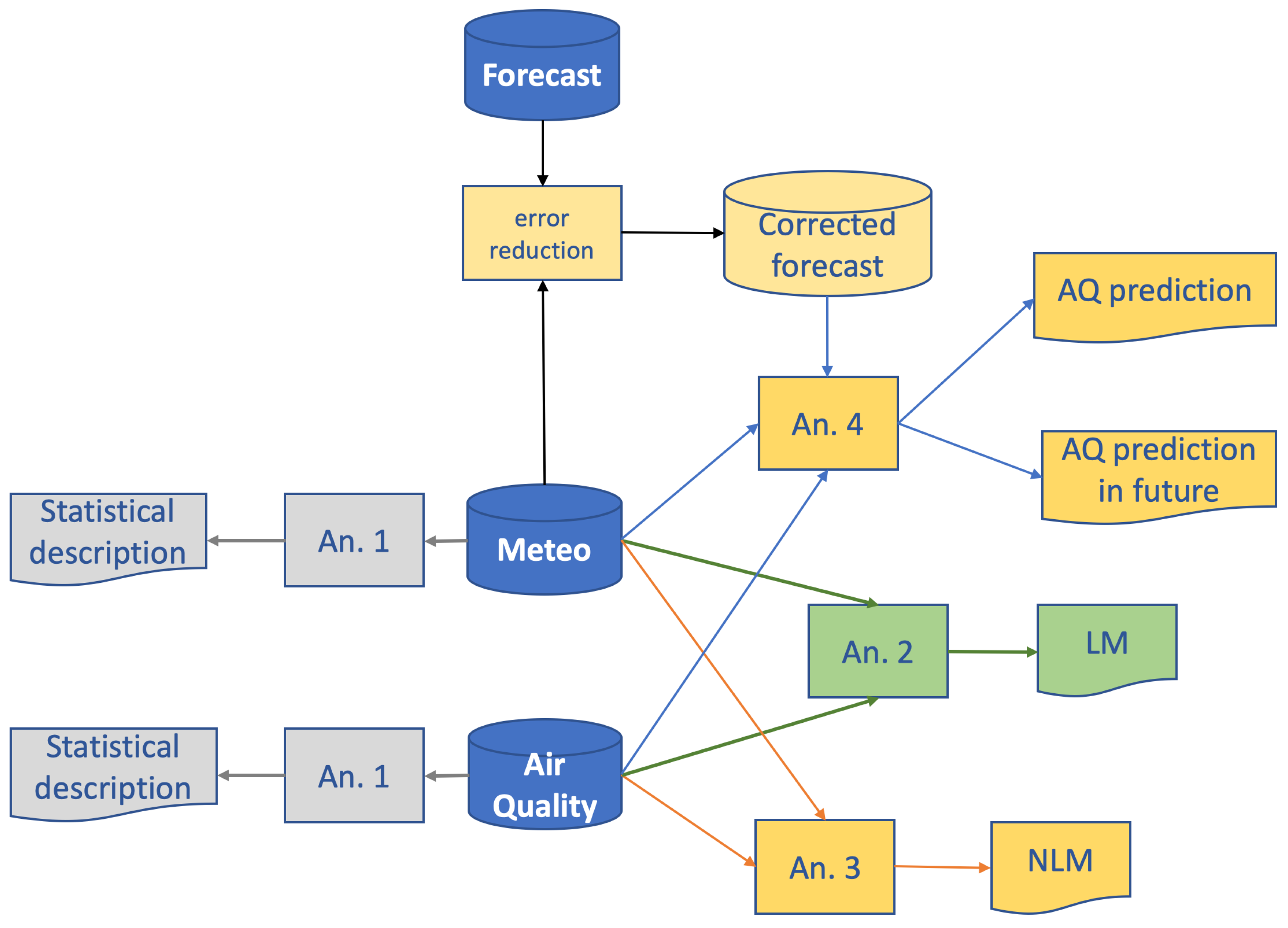
2. Materials and Methods
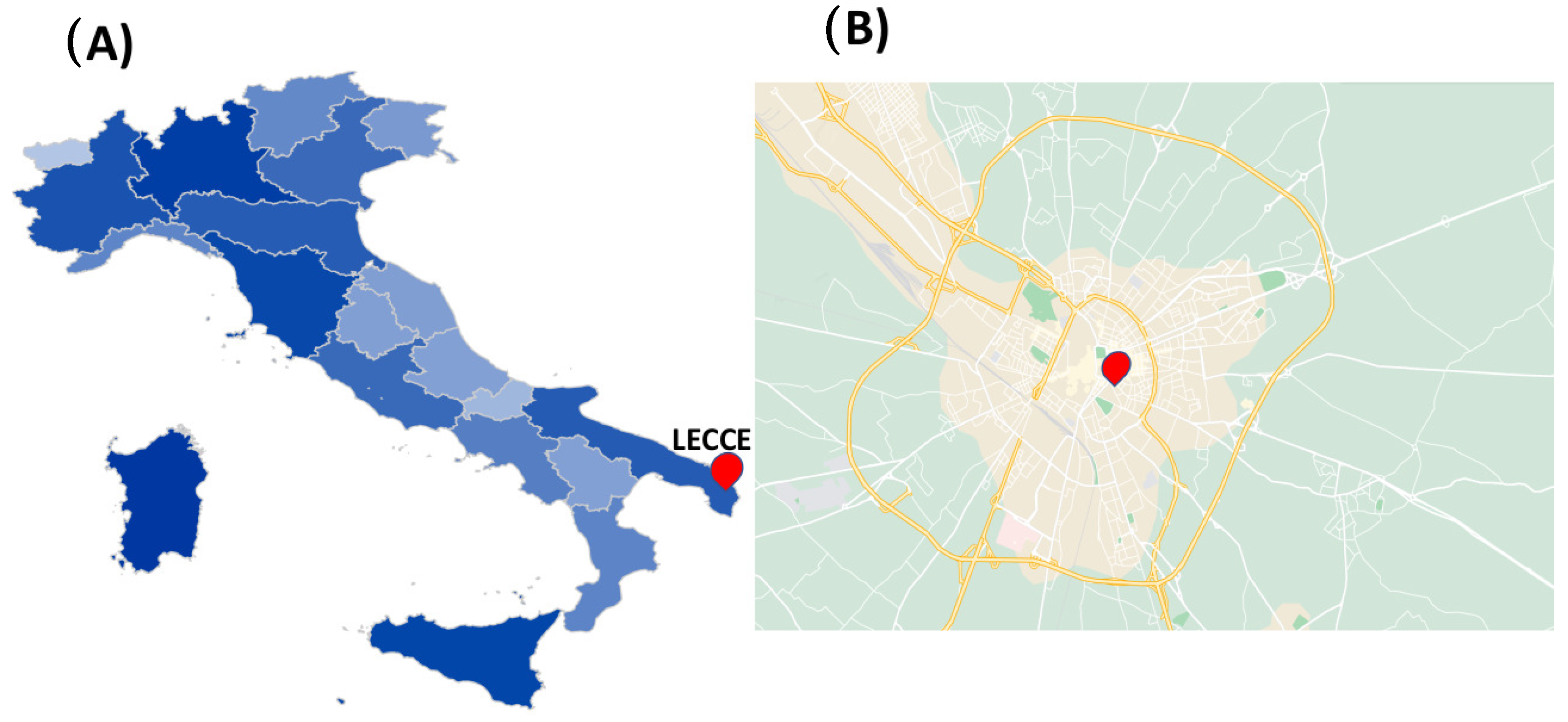
2.1. Data Collection
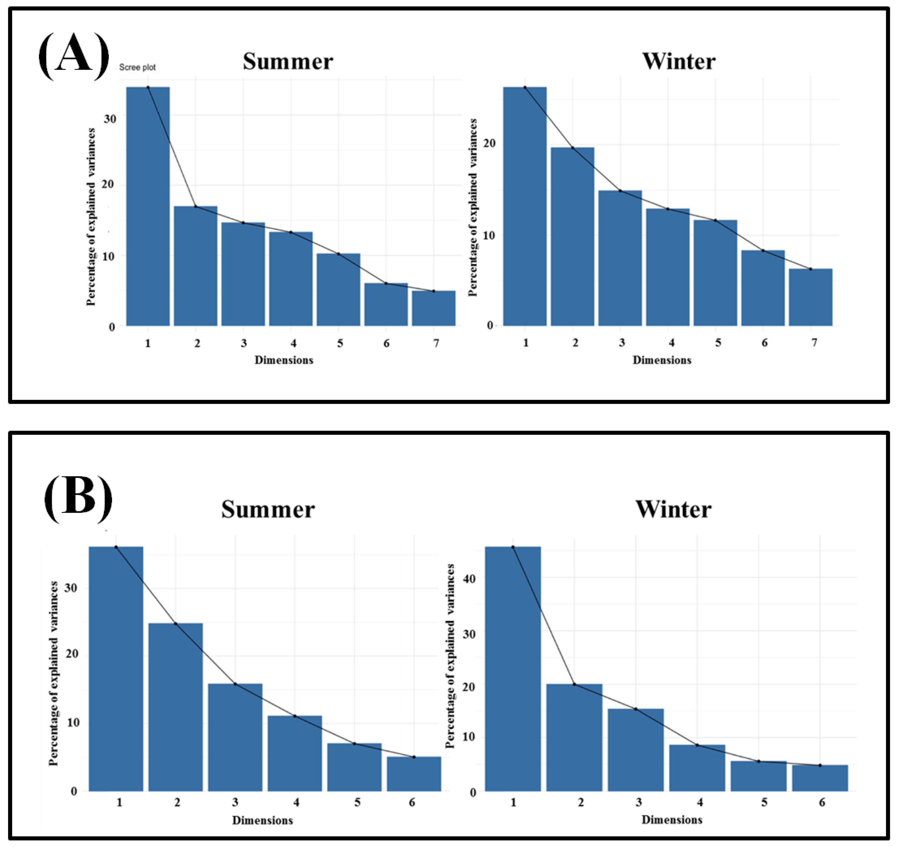
2.2. Exploratory Analysis
2.3. Linear Dependencies
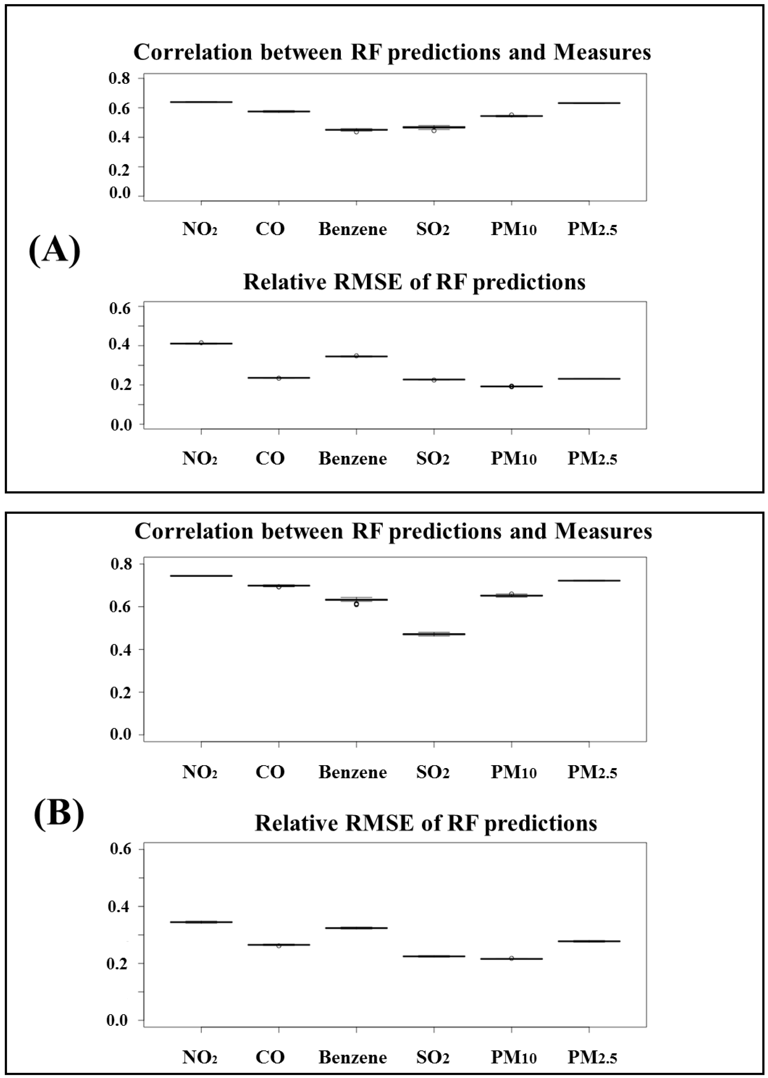
2.4. Machine Learning
2.5. Air Quality Predictions
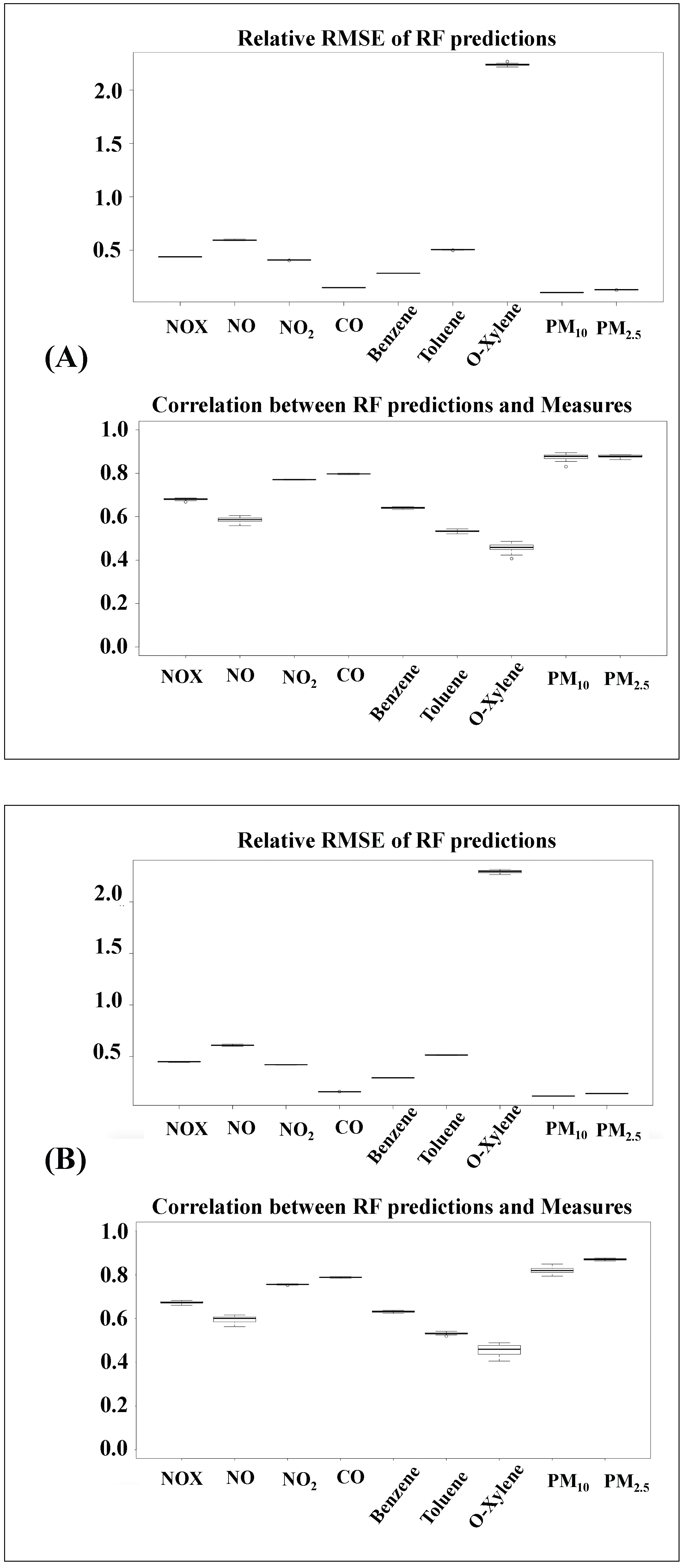
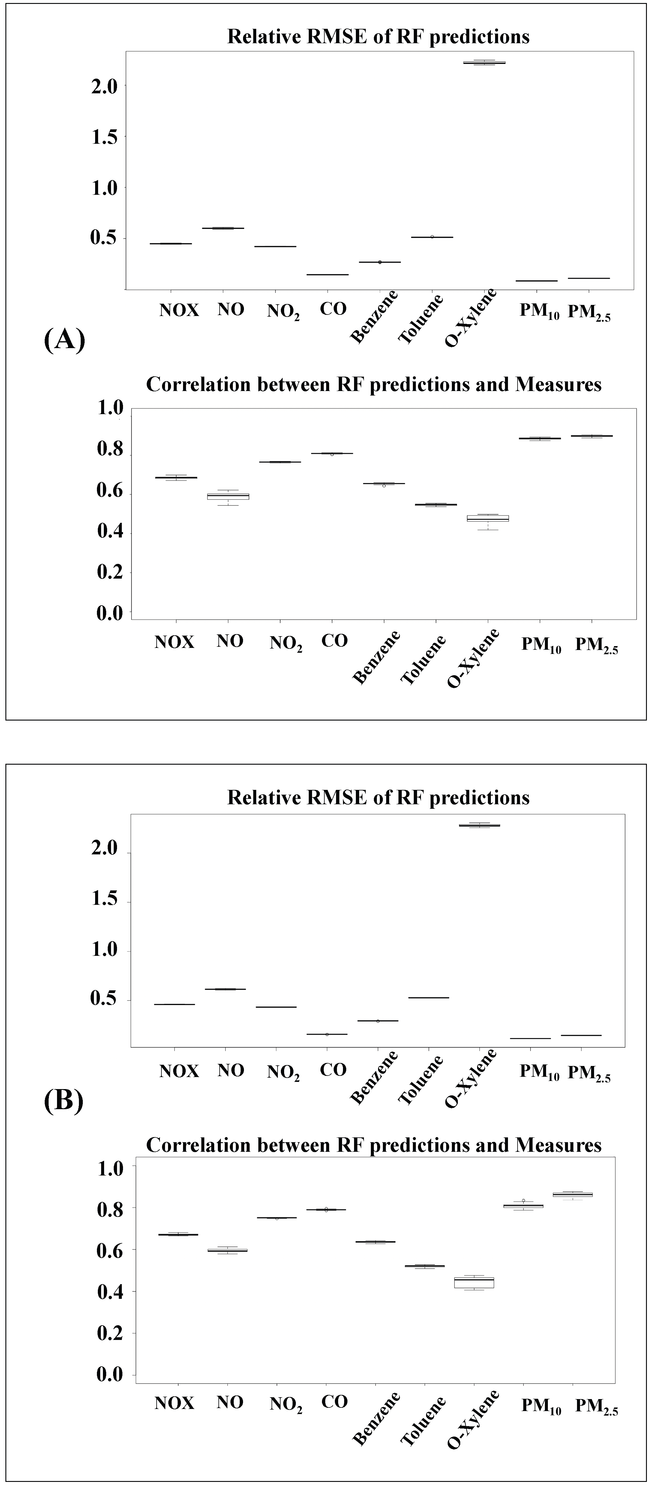
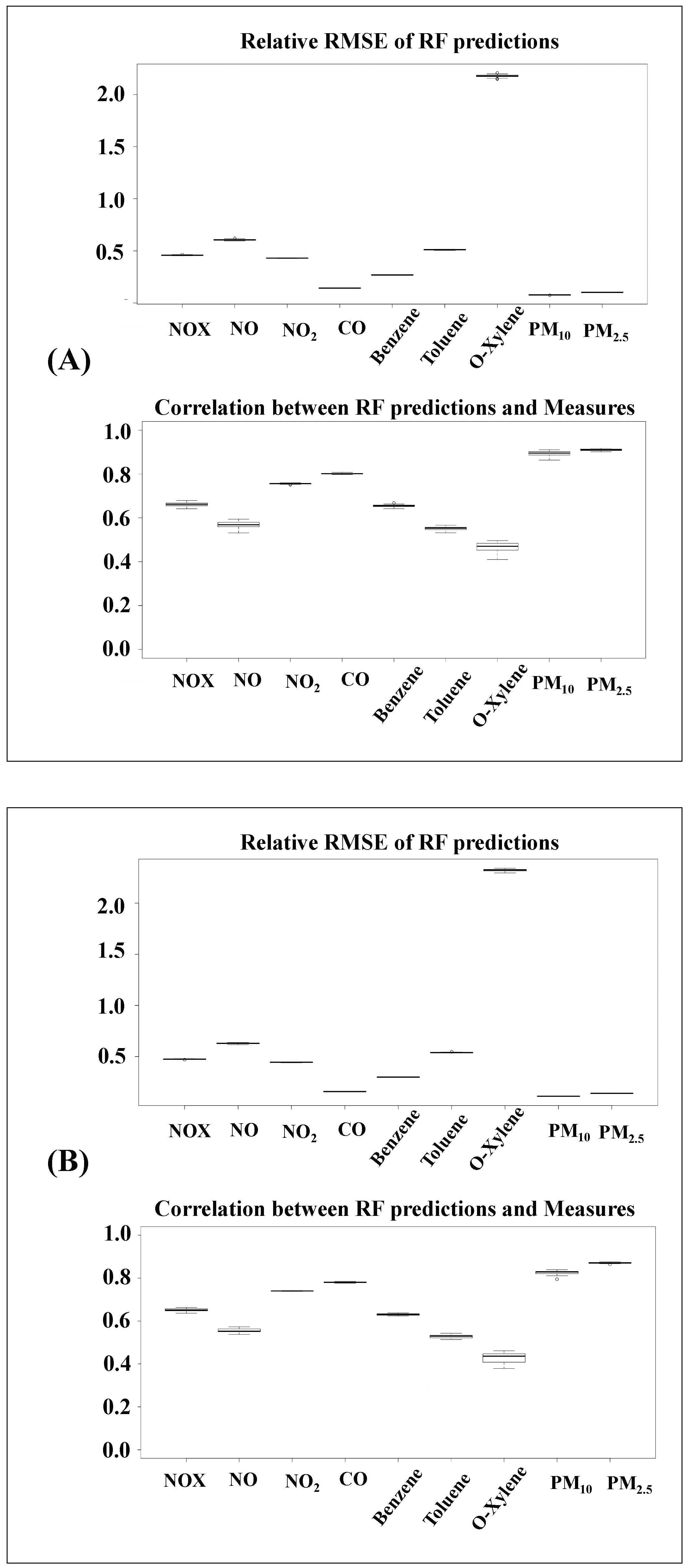
3. Results and Discussion
3.1. Statistical Description of the Data
3.2. Insights from Linear Models
3.3. Insights from Non-Linear Models
3.4. Air Quality Data Predictions
4. Conclusions
Supplementary Materials
Author Contributions
Funding
Conflicts of Interest
References
- Lionetto, M.G.; Guascito, M.R.; Caricato, R.; Giordano, M.E.; De Bartolomeo, A.R.; Romano, M.P.; Conte, M.; Dinoi, A.; Contini, D. Correlation of oxidative potential with ecotoxicological and cytotoxicological potential of PM10 at an urban background site in Italy. Atmosphere 2019, 10, 733. [Google Scholar] [CrossRef]
- Pope III, C.A.; Dockery, D.W. Health effects of fine particulate air pollution: Lines that connect. J. Air Waste Manag. Assoc. 2006, 56, 709–742. [Google Scholar] [CrossRef] [PubMed]
- Gualtieri, M.; Longhin, E.; Mattioli, M.; Mantecca, P.; Tinaglia, V.; Mangano, E.; Proverbio, M.C.; Bestetti, G.; Camatini, M.; Battaglia, C. Gene expression profiling of A549 cells exposed to Milan PM2.5. Toxicol. Lett. 2012, 209, 136–145. [Google Scholar] [CrossRef] [PubMed]
- Gauderman, W.J.; Urman, R.; Avol, E.; Berhane, K.; McConnell, R.; Rappaport, E.; Chang, R.; Lurmann, F.; Gilliland, F. Association of improved air quality with lung development in children. N. Engl. J. Med. 2015, 372, 905–913. [Google Scholar] [CrossRef] [PubMed]
- Velali, E.; Papachristou, E.; Pantazaki, A.; Choli-Papadopoulou, T.; Planou, S.; Kouras, A.; Manoli, E.; Besis, A.; Voutsa, D.; Samara, C. Redox activity and in vitro bioactivity of the water-soluble fraction of urban particulate matter in relation to particle size and chemical composition. Environ. Pollut. 2016, 208, 774–786. [Google Scholar] [CrossRef]
- Perrone, M.G.; Gualtieri, M.; Ferrero, L.; Porto, C.L.; Udisti, R.; Bolzacchini, E.; Camatini, M. Seasonal variations in chemical composition and in vitro biological effects of fine PM from Milan. Chemosphere 2010, 78, 1368–1377. [Google Scholar] [CrossRef]
- Happo, M.; Markkanen, A.; Markkanen, P.; Jalava, P.; Kuuspalo, K.; Leskinen, A.; Sippula, O.; Lehtinen, K.; Jokiniemi, J.; Hirvonen, M.R. Seasonal variation in the toxicological properties of size-segregated indoor and outdoor air particulate matter. Toxicol. Vitr. 2013, 27, 1550–1561. [Google Scholar] [CrossRef]
- Jia, Y.Y.; Wang, Q.; Liu, T. Toxicity research of PM2.5 compositions in vitro. Int. J. Environ. Res. Public Health 2017, 14, 232. [Google Scholar] [CrossRef]
- Li, N.; Sioutas, C.; Cho, A.; Schmitz, D.; Misra, C.; Sempf, J.; Wang, M.; Oberley, T.; Froines, J.; Nel, A. Ultrafine particulate pollutants induce oxidative stress and mitochondrial damage. Environ. Health Perspect. 2003, 111, 455–460. [Google Scholar] [CrossRef]
- Delfino, R.J.; Staimer, N.; Tjoa, T.; Gillen, D.L.; Schauer, J.J.; Shafer, M.M. Airway inflammation and oxidative potential of air pollutant particles in a pediatric asthma panel. J. Expo. Sci. Environ. Epidemiol. 2013, 23, 466–473. [Google Scholar] [CrossRef]
- Michael, S.; Montag, M.; Dott, W. Pro-inflammatory effects and oxidative stress in lung macrophages and epithelial cells induced by ambient particulate matter. Environ. Pollut. 2013, 183, 19–29. [Google Scholar] [CrossRef]
- Donaldson, K.; Stone, V.; Borm, P.J.; Jimenez, L.A.; Gilmour, P.S.; Schins, R.P.; Knaapen, A.M.; Rahman, I.; Faux, S.P.; Brown, D.M.; et al. Oxidative stress and calcium signaling in the adverse effects of environmental particles (PM10). Free Radic. Biol. Med. 2003, 34, 1369–1382. [Google Scholar] [CrossRef]
- Brugha, R.; Grigg, J. Urban air pollution and respiratory infections. Paediatr. Respir. Rev. 2014, 15, 194–199. [Google Scholar] [CrossRef]
- Kleine Deters, J.; Zalakeviciute, R.; Gonzalez, M.; Rybarczyk, Y. Modeling PM2.5 urban pollution using machine learning and selected meteorological parameters. J. Electr. Comput. Eng. 2017, 2017, 5106045. [Google Scholar] [CrossRef]
- World Health Organization. Air Pollution Levels Rising in Many of the World’s Poorest Cities. 2016. Available online: https://www.who.int/news/item/12-05-2016-air-pollution-levels-rising-in-many-of-the-world-s-poorest-cities (accessed on 10 October 2022).
- Lelieveld, J.; Evans, J.S.; Fnais, M.; Giannadaki, D.; Pozzer, A. The contribution of outdoor air pollution sources to premature mortality on a global scale. Nature 2015, 525, 367–371. [Google Scholar] [CrossRef]
- Xing, Y.F.; Xu, Y.H.; Shi, M.H.; Lian, Y.X. The impact of PM2.5 on the human respiratory system. J. Thorac. Dis. 2016, 8, E69. [Google Scholar]
- Carugno, M.; Dentali, F.; Mathieu, G.; Fontanella, A.; Mariani, J.; Bordini, L.; Milani, G.P.; Consonni, D.; Bonzini, M.; Bollati, V.; et al. PM10 exposure is associated with increased hospitalizations for respiratory syncytial virus bronchiolitis among infants in Lombardy, Italy. Environ. Res. 2018, 166, 452–457. [Google Scholar] [CrossRef]
- Conticini, E.; Frediani, B.; Caro, D. Can atmospheric pollution be considered a co-factor in extremely high level of SARS-CoV-2 lethality in Northern Italy? Environ. Pollut. 2020, 261, 114465. [Google Scholar] [CrossRef]
- Sciomer, S.; Moscucci, F.; Magrì, D.; Badagliacca, R.; Piccirillo, G.; Agostoni, P. SARS-CoV-2 spread in Northern Italy: What about the pollution role? Environ. Monit. Assess. 2020, 192, 325. [Google Scholar] [CrossRef]
- Setti, L.; Passarini, F.; De Gennaro, G.; Barbieri, P.; Pallavicini, A.; Ruscio, M.; Piscitelli, P.; Colao, A.; Miani, A. Searching for SARS-COV-2 on Particulate Matter: A Possible Early Indicator of COVID-19 Epidemic Recurrence. Int. J. Environ. Res. Public Health. 2020, 17, 2986. [Google Scholar] [CrossRef]
- Gatti, R.C.; Velichevskaya, A.; Tateo, A.; Amoroso, N.; Monaco, A. Machine learning reveals that prolonged exposure to air pollution is associated with SARS-CoV-2 mortality and infectivity in Italy. Environ. Pollut. 2020, 267, 115471. [Google Scholar] [CrossRef] [PubMed]
- Ciencewicki, J.; Jaspers, I. Air pollution and respiratory viral infection. Inhal. Toxicol. 2007, 19, 1135–1146. [Google Scholar] [CrossRef] [PubMed]
- Wong, C.M.; Thach, T.Q.; Chau, P.; Chan, E.; Chung, R.Y.n.; Ou, C.Q.; Yang, L.; Peiris, J.; Thomas, G.N.; Lam, T.H.; et al. Part 4. Interaction between Air Pollution and Respiratory Viruses: Time-Series Study of Daily Mortality and Hospital Admissions in Hong Kong; Research Report; Health Effects Institute: Boston, MA, USA, 2010; pp. 283–362. [Google Scholar]
- Nenna, R.; Evangelisti, M.; Frassanito, A.; Scagnolari, C.; Pierangeli, A.; Antonelli, G.; Nicolai, A.; Arima, S.; Moretti, C.; Papoff, P.; et al. Respiratory syncytial virus bronchiolitis, weather conditions and air pollution in an Italian urban area: An observational study. Environ. Res. 2017, 158, 188–193. [Google Scholar] [CrossRef] [PubMed]
- Ramsey, N.R.; Klein, P.M.; Moore, B. The impact of meteorological parameters on urban air quality. Atmos. Environ. 2014, 86, 58–67. [Google Scholar] [CrossRef]
- Wang, J.; Ogawa, S. Effects of meteorological conditions on PM2.5 concentrations in Nagasaki, Japan. Int. J. Environ. Res. Public Health 2015, 12, 9089–9101. [Google Scholar] [CrossRef]
- Zhang, F.; Cheng, H.r.; Wang, Z.w.; Lv, X.p.; Zhu, Z.m.; Zhang, G.; Wang, X.m. Fine particles (PM2.5) at a CAWNET background site in Central China: Chemical compositions, seasonal variations and regional pollution events. Atmos. Environ. 2014, 86, 193–202. [Google Scholar] [CrossRef]
- Li, Y.; Chen, Q.; Zhao, H.; Wang, L.; Tao, R. Variations in PM10, PM2.5 and PM1.0 in an urban area of the Sichuan Basin and their relation to meteorological factors. Atmosphere 2015, 6, 150–163. [Google Scholar] [CrossRef]
- Lombardi, A.; Diacono, D.; Amoroso, N.; Monaco, A.; Tavares, J.M.R.; Bellotti, R.; Tangaro, S. Explainable deep learning for personalized age prediction with brain morphology. Front. Neurosci. 2021, 15, 578. [Google Scholar] [CrossRef]
- Amoroso, N.; Pomarico, D.; Fanizzi, A.; Didonna, V.; Giotta, F.; La Forgia, D.; Latorre, A.; Monaco, A.; Pantaleo, E.; Petruzzellis, N.; et al. A roadmap towards breast cancer therapies supported by explainable artificial intelligence. Appl. Sci. 2021, 11, 4881. [Google Scholar] [CrossRef]
- Tateo, A.; Miglietta, M.M.; Fedele, F.; Menegotto, M.; Monaco, A.; Bellotti, R. Ensemble using different Planetary Boundary Layer schemes in WRF model for wind speed and direction prediction over Apulia region. Adv. Sci. Res. 2017, 14, 95–102. [Google Scholar] [CrossRef]
- Fedele, F.; Miglietta, M.M.; Perrone, M.R.; Burlizzi, P.; Bellotti, R.; Conte, D.; Carducci, A.G.C. Numerical simulations with the WRF model of water vapour vertical profiles: A comparison with LIDAR and radiosounding measurements. Atmos. Res. 2015, 166, 110–119. [Google Scholar] [CrossRef]
- Berman, F.; Chien, A.; Cooper, K.; Dongarra, J.; Foster, I.; Gannon, D.; Johnsson, L.; Kennedy, K.; Kesselman, C.; Mellor-Crumme, J.; et al. The GrADS project: Software support for high-level grid application development. Int. J. High Perform. Comput. Appl. 2001, 15, 327–344. [Google Scholar] [CrossRef]
- Abdi, H.; Williams, L.J. Principal component analysis. Wiley Interdiscip. Rev. Comput. Stat. 2010, 2, 433–459. [Google Scholar] [CrossRef]
- Meuzelaar, H.; Statheropoulos, M.; Huai, H.; Yun, Y. Canonical Correlation Analysis of Multisource Fossil Fuel Data. Comput.-Enhanc. Anal. Spectrosc. Peter A. Jurs Plenum Publ. 1992, 111, 185–213. [Google Scholar]
- Statheropoulos, M.; Vassiliadis, N.; Pappa, A. Principal component and canonical correlation analysis for examining air pollution and meteorological data. Atmos. Environ. 1998, 32, 1087–1095. [Google Scholar] [CrossRef]
- Breiman, L. Random forests. Mach. Learn. 2001, 45, 5–32. [Google Scholar] [CrossRef]
- Tateo, A.; Bellotti, R.; Fedele, F.; Guarnieri Calò Carducci, A.; Pollice, A. Post-processing of the Weather Research and Forecasting (WRF) Mesoscale Model by Artificial Neural Networks. In Proceedings of the GRASPA-SIS Biennial Conference, Bari, Italy, 15–16 June 2015. [Google Scholar]


| Meteorological Data | |||||||
|---|---|---|---|---|---|---|---|
| Median | T. max | UMR min | Prec. | WS max | WD prev. | Rad.mean | Press Atm |
| SUMMER | |||||||
| WINTER | |||||||
| Air Quality Data | ||||||
|---|---|---|---|---|---|---|
| Median | Benzene | |||||
| SUMMER | ||||||
| WINTER | ||||||
| SUMMER | |||||||
|---|---|---|---|---|---|---|---|
| Correlation coefficient | T.max | UMR | Prec | WS | WD. | RAD | . Press.Atm. |
| −0.16 | 0.04 | 0.02 | −0.27 | −0.05 | −0.19 | −0.00 | |
| −0.17 | 0.05 | 0.00 | −0.22 | −0.04 | −0.13 | 0.04 | |
| −0.08 | 0.09 | 0.01 | −0.22 | −0.03 | −0.08 | 0.08 | |
| 0.22 | −0.09 | −0.02 | 0.04 | 0.01 | 0.15 | 0.03 | |
| 0.28 | −0.14 | −0.05 | −0.07 | −0.04 | 0.01 | 0.08 | |
| 0.27 | −0.07 | −0.03 | −0.19 | −0.06 | 0.03 | 0.28 | |
| WINTER | |||||||
| Correlation coefficient | T.max | UMR | Prec | WS | WD. | RAD | . Press.Atm. |
| −0.14 | 0.09 | −0.04 | −0.39 | 0.01 | −0.23 | 0.08 | |
| −0.25 | 0.04 | −0.06 | −0.32 | 0.03 | −0.16 | 0.14 | |
| −0.18 | 0.06 | −0.06 | −0.32 | 0.06 | −0.14 | 0.18 | |
| 0.00 | −0.06 | 0.01 | −0.01 | 0.01 | 0.08 | 0.01 | |
| 0.09 | 0.03 | −0.06 | −0.15 | 0.02 | 0.03 | 0.24 | |
| −0.13 | −0.02 | −0.08 | −0.32 | 0.08 | 0.03 | 0.44 | |
| Linear Model | ||||||
|---|---|---|---|---|---|---|
| Correlation Coefficient | ||||||
| SUMMER | 0.32 | 0.27 | 0.23 | 0.24 | 0.34 | 0.44 |
| WINTER | 0.41 | 0.37 | 0.36 | 0.10 | 0.30 | 0.50 |
| Canonical Component Analysis | ||||||
|---|---|---|---|---|---|---|
| CC-1 | CC-2 | CC-3 | CC-4 | CC-5 | CC-6 | |
| SUMMER | 0.47 | 0.37 | 0.25 | 0.11 | 0.05 | 0.03 |
| WINTER | 0.57 | 0.38 | 0.29 | 0.09 | 0.04 | 0.03 |
| Random Forest | ||||||
|---|---|---|---|---|---|---|
| Correlation Coefficient | ||||||
| SUMMER | 0.93 | 0.94 | 0.93 | 0.94 | 0.95 | 0.94 |
| WINTER | 0.92 | 0.92 | 0.92 | 0.93 | 0.94 | 0.93 |
Disclaimer/Publisher’s Note: The statements, opinions and data contained in all publications are solely those of the individual author(s) and contributor(s) and not of MDPI and/or the editor(s). MDPI and/or the editor(s) disclaim responsibility for any injury to people or property resulting from any ideas, methods, instructions or products referred to in the content. |
© 2023 by the authors. Licensee MDPI, Basel, Switzerland. This article is an open access article distributed under the terms and conditions of the Creative Commons Attribution (CC BY) license (https://creativecommons.org/licenses/by/4.0/).
Share and Cite
Tateo, A.; Campanaro, V.; Amoroso, N.; Bellantuono, L.; Monaco, A.; Pantaleo, E.; Rinaldi, R.; Maggipinto, T. Predicting Air Quality from Measured and Forecast Meteorological Data: A Case Study in Southern Italy. Atmosphere 2023, 14, 475. https://doi.org/10.3390/atmos14030475
Tateo A, Campanaro V, Amoroso N, Bellantuono L, Monaco A, Pantaleo E, Rinaldi R, Maggipinto T. Predicting Air Quality from Measured and Forecast Meteorological Data: A Case Study in Southern Italy. Atmosphere. 2023; 14(3):475. https://doi.org/10.3390/atmos14030475
Chicago/Turabian StyleTateo, Andrea, Vincenzo Campanaro, Nicola Amoroso, Loredana Bellantuono, Alfonso Monaco, Ester Pantaleo, Rosaria Rinaldi, and Tommaso Maggipinto. 2023. "Predicting Air Quality from Measured and Forecast Meteorological Data: A Case Study in Southern Italy" Atmosphere 14, no. 3: 475. https://doi.org/10.3390/atmos14030475
APA StyleTateo, A., Campanaro, V., Amoroso, N., Bellantuono, L., Monaco, A., Pantaleo, E., Rinaldi, R., & Maggipinto, T. (2023). Predicting Air Quality from Measured and Forecast Meteorological Data: A Case Study in Southern Italy. Atmosphere, 14(3), 475. https://doi.org/10.3390/atmos14030475