Article

Possible Pre-Seismic Indications Prior to Strong Earthquakes That Occurred in Southeastern Mediterranean as Observed Simultaneously by Three VLF/LF Stations Installed in Athens (Greece)

by
Dimitrios Z. Politis
1,
Stelios M. Potirakis
1,2,*,
Sudipta Sasmal
3,
Filopimin Malkotsis
1,4,
Dionisis Dimakos
4 and
Masashi Hayakawa
5,6
1
Department of Electrical and Electronics Engineering, University of West Attica, Ancient Olive Grove Campus, 12241 Aigaleo, Greece
2
Institute for Astronomy, Astrophysics, Space Applications and Remote Sensing, National Observatory of Athens, Metaxa and Vasileos Pavlou, 15236 Penteli, Greece
3
Institute of Astronomy Space and Earth Science, AJ 316, Sector II, Salt Lake, Kolkata 700091, India
4
Hellenic Telecommunications and Post Commission (EETT), 60 Kifissias Avenue, 15125 Marousi, Greece
5
Hayakawa Institute of Seismo-Electromagnetics Co. Ltd. (Hi-SEM), University of Electro-Communications (UEC) Alliance Center #521, 1-1-1 Kojimacho, Chofu, Tokyo 1820026, Japan
6
Advanced Wireless and Communications Research Center (AWCC), University of Electro-Communications (UEC), 1-5-1 Chofugaoka, Chofu, Tokyo 1828585, Japan
*
Author to whom correspondence should be addressed.
Atmosphere 2023, 14(4), 673; https://doi.org/10.3390/atmos14040673
Submission received: 5 March 2023 / Revised: 26 March 2023 / Accepted: 29 March 2023 / Published: 1 April 2023
(This article belongs to the Special Issue Recent Advances in Ionosphere Observation and Investigation)

Abstract

:
In this work, we present the analysis of VLF/LF sub-ionospheric propagation data to study anomalies possibly related to very recent strong (M > 5.5) earthquakes (EQs) that occurred in the southeastern Mediterranean in September–October 2021 and January 2022. We used the signal of one transmitter located at Negev in Israel (29.7 kHz) as received by three VLF/LF receivers (two of them using identical SW and HW) installed, at a close distance to each other, in Athens (Greece). This study employed multiple methods and techniques to analyze the reception amplitude data to identify any possible EQ-related anomalies. More specifically, first, we used both statistical and criticality analysis methods such as the “nighttime fluctuation method” (NFM), the “terminator time method” (TTM), and the “natural time” (NT) analysis method. These methods have satisfactorily been applied in the past in a series of other studies leading to interesting results. Moreover, we additionally used two more analysis techniques focusing on the signal’s amplitude characteristics. The first is the wavelet analysis of the nighttime part of the signal’s amplitude. It is based on the Morlet wavelet function, aiming to unveil the possible existence of atmospheric gravity waves (AGWs) before EQ. The second is named “long wavelength propagation capability” (LWPC), which simulates the amplitude of the signal and is based on the reflection parameters of ionosphere and by searching for increases or decreases of the electron density profile of the ionospheric D layer concerning the shifts of the minima of terminator times (TTs) in the diurnal variation of the signal. Finally, in this work, we summarize our findings and discuss possible “pre-”, “co-”, and “post-” seismic effects as observed from all the work.

1. Introduction

The very-low- to low-frequency (VLF/LF) monitoring of the lower ionosphere is an effective and simple technique for probing this part of the atmosphere, especially for detecting ionospheric disturbances caused by various terrestrial and extra-terrestrial extreme events, e.g., [1,2,3,4]. More and more researchers and amateur radio engineers have shown great interest in installing VLF/LF recording systems (receivers) at different places worldwide to observe and understand these extreme events, e.g., [1,2,3,4,5,6,7,8]. More specifically, seismo-ionospheric studies are the most controversial among many scientists [1]. However, a unified and well-established theoretical pre-seismic model that shows the linkage of three specific planetary layers is called “lithosphere–atmosphere–ionosphere coupling” (LAIC) [1]. This model clearly describes the physical processes behind the preparation of an impending earthquake (EQ), but it is still poorly understood at the moment [1]. Considering those physical mechanisms, this model separates the different observable quantities by grouping them into five suggested channels. These are electromagnetic (EM), chemical, thermal, electrostatic, and acoustic [1,9].
On the other hand, other observed EM quantities have also been used to unveil EQ-related signatures prior to EQs. For example, these are kHz–MHz fracto-electromagnetic (fracto-EM) emissions, ultra-low-frequency (ULF) magnetic field data, and seismic electric signals (SES) [10,11,12,13]. Specifically, to these observed EM quantities, different methods and techniques from the theory of complex systems have been applied in past studies by examining in this manner other characteristics of the signal (and the system of which these are observables), such as the information content, fractality, and criticality, e.g., [10,11,12,13].
For VLF/LF sub-ionospheric propagation data, two well-established criticality analysis methods have been applied. Specifically, these are “the method of critical fluctuations” (MCF) and the “natural time” (NT) analysis, which can unveil the approach of criticality; they have been applied to the case of the 2016 Kumamoto EQs and 2020 Samos EQ [8,14,15]. However, there are differences in the application of these two methods. The first one was applied to the raw amplitude recordings. In contrast, the second one was used on the three statistical quantities of the “nighttime fluctuation method,” which is based on the raw amplitude recordings of the VLF/LF signal [8,14,15].
A second statistical method called the “terminator time method” (TTM) is very important for the detection of shifts of the terminator times (TTs), which appear as minima around the planetary sunrise and sunset time, before the occurrence of an EQ [16]. This behavior of shifts of TTs was first reported in Japan in 1995 before the famous Kobe EQ (M7.1) [16]. In two recent studies of the 2020 Samos EQ, significant shifts of TTs have been observed towards night for two studied sub-ionospheric propagation paths. They have been characterized as possible anomalous shifts prior to the EQ [8,17].
A conventional technique for the analysis of VLF/LF nighttime amplitude recordings is the “wavelet analysis” technique, which is based on the Morlet wavelet function, aiming to unveil the possible existence of atmospheric gravity waves (AGW) prior to an EQ [18,19,20,21]. These anomalies of AGW appear as periodic structures in the VLF amplitude recordings [19,20,21]. More specifically, anomalies associated with AGW have been observed, for example, before the 2016 Imphal EQ in India, where signatures of periodic structures were revealed with a periodicity of ~60 min [19].
Another simple and well-established technique for searching ionospheric anomalies before EQs by simulating the VLF amplitude recordings is called the “long wavelength propagation capability” (LWPC) [22]. Specifically, this technique simulates the amplitude and phase of the signal by knowing the location of the transmitter and the receiver at any place on earth. This technique treats the earth and the lower ionosphere as a waveguide by using single or multiple reflections to guide an emitted VLF/LF signal based on the sub-ionospheric propagation characteristics of the propagation path. Besides the signal’s amplitude and phase simulation, another essential factor is the calculation of the lower ionosphere’s electron density (ED) profile for a given location and time. By knowing that the radio signals use the D and E layers to be transmitted, they are affected by them.
Many extreme events can disturb the lower ionosphere, such as EQs, solar flares, and geomagnetic storms, by changing locally or globally the ED profile [17,23,24,25]. However, the calculation of the ED profile is achieved by two significant parameters in LWPC, which are called the “steepness parameter” ( β ) and “ionospheric reflection height” ( h ), taken from the theory of Wait’s exponential ED profile [26,27]. For the 2020 Samos EQ, pre-EQ shifts of TTs have been observed as pre-seismic indications [17]. By numerically simulating around those TTs, by taking into account a small excerpt of the signal’s amplitude, the simulated profile was reproduced at the receiver’s location with proper corroboration with its observed profile (amplitude recordings) [17]. Using Wait’s exponential formula for a particular set, the ED profile was calculated precisely at the time of occurrence of the minima of the shifted TTs. In that work, increases or decreases in the ED profile were generally observed as possible pre-seismic indications before the 2020 Samos EQ [17].
By taking into account all those mentioned above, in this work, we used all these described methods and techniques to search for pre-EQ ionospheric anomalies in the VLF amplitude recordings during strong ( M L 5.5 ) EQs that occurred in the southeastern Mediterranean in September and October of 2021, as well as in January of 2022. The first case concerns three EQs that occurred in September and October of 2021 and hit Crete Island (Greece), causing several damages, or occurred close to Crete, M L 5.8 on 27 September 2021, M L 6.3 on 12 October 2021, and M L 6.1 on 19 October 2021, hereafter referred to as “the 2021 Crete EQs” (please see more information in Section 2). The second case concerns an EQ that hit a sea area northwest of Cyprus Island on January of 2022, M L 6.4 on11 January 2022, due to which no damage was reported, hereafter referred to as “the 2022 Cyprus EQ” (please see more information in Section 2). In our study, we utilized three VLF/LF receivers located in Athens (Greece) to study these EQs [2,8]. These VLF/LF receivers have recently been established searching for ionospheric perturbations caused by various extraterrestrial or terrestrial phenomena, but especially for studying EQs [2,8]. The first one has been operating since March 2020, while the two other identical VLF/LF stations, having different hardware and software from the initial, were installed in June and September of 2021, respectively [2,8].
In the first part of this study, we analyze the raw amplitude recordings of the signal from the three stations using statistical methods such as NFM and TTM. At the same time, we use one criticality analysis method called the “NT analysis method” to analyze the three statistical quantities of NFM. Then, any statistical anomalies and criticality signatures possibly correlated with the EQs under study are searched for a period of 15 days before each of them. In addition, we analyze the raw amplitude data using the “Morlet wavelet analysis searching for AGWs”. The results of identified perturbations in the VLF/LF amplitude recordings caused by AGWs are unveiled in 32 to 128 min and in 15 days before each one of the studied EQs. Moreover, in this work, we include the LWPC technique by numerically simulating the amplitude recordings and selecting a small excerpt of the signal where TTs exist. Anomalies associated with increases or decreases in ED according to the shifted TTs are revealed 15 days before each studied EQ (2021 Crete EQs, 2022 Cyprus EQ).
By understanding all those mentioned above, the structure of this manuscript is the following. In the Section 2 of this manuscript, we give details about the sub-ionospheric propagation data, the EQs under study, and other possibly ionosphere-influencing extreme events. In the Section 3, we briefly describe the methods and techniques used for this study. In the Section 4, we present the results; finally, in the Section 5, we give conclusions about the whole study.

2. Sub-Ionospheric Propagation Data, Studied EQs, and Other Non-Examined Extreme Events

This section gives detailed information about the VLF/LF receivers used in our study and the characteristics of VLF/LF sub-ionospheric propagation data. For this study, we choose one transmitter (call sign: ISR), which is located at Negev (37.4094° N, 27.3252° E) in Israel, and its transmitted frequency is 29.7 kHz, while the reception of the signal is conducted by three VLF/LF stations, all located in the prefecture of Attica in Greece. More specifically, two of the three VLF/LF receivers have the same features. The first one is located in a forest area (38.0317° N, 23.6637° E) to the west of Athens, called Aspra Chomata (call sign: ACH), close to the urban complex of Athens, while the second one is located in a suburban area (38.0317° N, 23.8572° E) to the east of Athens, called Gerakas (call sign: GER). At this point, it is noted that these two receivers were recently installed in June and September of 2021, respectively, and they are operating with 30 s sampling. These two receivers can record signals up to 100 kHz, and the detailed description of the setup of their hardware and software and the recorded transmitters are presented in detail in [2].
On the other hand, the third VLF/LF receiver is located at the University of West Attica (call sign: UWA) in the prefecture of Attica in Athens (Greece) and has different features from the other two abovementioned VLF/LF receivers; this receiver has a sampling frequency of 1 s and records frequencies up to 47.5 kHz. The information about the monitored transmitters and key information about this VLF/LF receiver are given in [8]. In addition, a detailed description of the hardware and software is provided on the UltraMSK website (https://www.ultramsk.com (accessed on 29 November 2022)). In Figure 1, we present a satellite image of the prefecture of Attica in Greece. The three VLF/LF stations are shown, together with the distances between each pair of receivers.
In Table 1, we give information about the EQs under study, taken from the seismic catalog of the National Observatory of Athens (NOA) (https://bbnet.gein.noa.gr/HL/databases/database) (accessed on 29 November 2022). All four of them took place in the southeastern Mediterranean from September to October 2021 and January 2022. Specifically, the EQs mentioned above are the 2021 Crete EQs and 2022 Cyprus EQ, which are indicated in this table in the column “EQ group”. Table 1 includes the EQ’s occurrence time, magnitude, depth, and coordinates of each epicenter. We should also mention that these EQs have a magnitude of 5.5 above, so they are expected to significantly perturb the lower ionosphere [1]. Moreover, we note that for this study, we search for EQ-related signatures within 15 days before each target EQ. In Figure 2, we show the map of the eastern Mediterranean where a representative fifth Fresnel zone of the sub-ionospheric propagation path is shown between each receiver and the transmitter ISR. The EQs chosen for this study are relatively close or within the fifth Fresnel zone of each monitored propagation path between the transmitter ISR and each receiver (UWA, ACH, and GER).
As already mentioned in Section 1, the ionosphere is sensitive to various extreme events occurring in the terrestrial, atmospheric, or space environment (e.g., earthquakes, volcanoes, typhoons, geomagnetic storms, solar flares, lighting activity, and weather storms), while it is not easy to indisputably attribute an ionospheric anomaly to a specific event if more than one of them are happening in close time distance. For this reason, we check our results against all recorded possibly ionosphere-influencing phenomena that occurred during the time periods of interest.
In this direction, we initially checked the geomagnetic conditions for each studied case (2021 Crete EQs and 2022 Cyprus EQ). For the 2021 Crete EQs, the corresponding geomagnetic indices Dst, Kp, ap, and Ap have been reported in a previous work [2]. Specifically, in Fig. 16 of ref. [2], two minor geomagnetic storms, of minimum Dst value ~−50 nT, happened on 17 September 2021 and 12 October 2021. At the same time, a simultaneous increase by exceeding an appropriate threshold (different for each index) is observed for the rest of the indices (Kp, ap, Ap).
Additionally, for the 2022 Cyprus EQ, the variation of geomagnetic indices (Dst, Kp, ap, Ap), as well as the peak flux ( W / m 2 ) of solar flares, are all shown in five panels for the period from 1 December 2021 until 15 February 2022. We have retrieved the data of Dst, Kp, ap, and Ap from the World Data Center for Geomagnetism of Kyoto (https://wdc.kugi.kyoto-u.ac.jp/wdc/Sec3.html (accessed on 29 November 2022)), while for solar flares we checked the data on solar X-ray flux from the National Oceanic and Atmospheric Administration (https://www.swpc.noaa.gov/products/goes-x-ray-flux (accessed on 29 November 2022)). As is evident from Figure 3, one moderate geomagnetic storm of −91 nT (min Dst) occurred on 14 January 2022, while a simultaneous enhancement (shown with red color) in the two geomagnetic indices (Kp, ap) appears for a very short time (one bin) period. Finally, in the bottom panel, we present all solar flares of the M and X classes that occurred in the abovementioned period. It can be observed that there were several solar flares of the M class in the entire period, but no X class solar flare.
However, other possibly ionosphere-influencing extreme events during the 2021 Crete EQs and 2022 Cyprus EQ have also been checked. We first checked the parameter of convective available potential energy (commonly abbreviated as CAPE) as an indication of atmospheric instability by observing its distribution on the map from the Ventusky search engine (https://www.ventusky.com (accessed on 29 November 2022)), the data of which are provided by the National Oceanic and Atmospheric Administration (NOAA) and the Deutscher Wetterdienst (DWD), while lightning activity was checked using the “Blitzortung.org” lightning-detection network (https://www.blitzortung.org/en/historical_maps.php (accessed on 29 November 2022)) and “lightningmaps.org” (https://www.lightningmaps.org/ (accessed on 29 November 2022)). However, no thunderstorms or typhoons were observed. Finally, the volcanic eruption database of the Global Volcanism Program of the Smithsonian Institution (https://volcano.si.edu/search_eruption.cfm (accessed on 29 November 2022)) was checked for possibly erupting volcanoes during the period of the studied EQs (2021 Crete EQs and 2022 Cyprus EQ), but no volcanic eruptions were recorded.
At this point, we should clarify that there were two strong events in the area of Crete Island that happened during the time period examined for the case of the 2022 Cyprus EQ (2 December 2021 29 January 2022). Both were of M L 5.5 according to the seismic catalog of NOA. Therefore, they may have affected the lower ionosphere. Specifically, these EQs occurred on 26 December 2021 18:59:02 UT, at (35.2029° N, 26.8497° Ε), within the fifth Fresnel zone of the examined paths, with a magnitude of 5.5 M L and a focal depth of 6.1 km, and on 29 December 2021 05:08:09 UT, at (34.791° N, 25.1303° Ε), out of the fifth Fresnel zone of the examined paths, with a magnitude of 5.7 M L and a focal depth of 67.1 km. Although for the specific studied period (2 December 2021 29 January 2022) we focus on the 2022 Cyprus EQ, we also check for perturbations possibly related to them.

3. Methods

In this section, we describe all the methods and techniques used in this study. Specifically, we present each method in a separate subsection as follows. In Section 3.1, we present the nighttime fluctuation method (NFM), while in Section 3.2, the terminator time method (TTM) is described. In Section 3.3, we present the natural time (NT) method, which can identify criticality before the occurrence of EQs. In Section 3.4, we show the wavelet analysis method for the VLF nighttime amplitude recordings. Finally, in Section 3.5, we discuss the “long wavelength propagation capability” (LWPC), which is a well-defined technique to simulate the electron density (ED) profile versus the ionospheric height at any time and anywhere on Earth based on the location of the transmitter and the receiver.

3.1. Nighttime Fluctuation Method (NFM)

The nighttime fluctuation method (NFM) was proposed for the detection of statistical anomalies caused by ionospheric disturbances concerning a variety of extreme events such as EQs [1,2]. First of all, the raw nighttime amplitude data (in dB) are extracted from the diurnal variation of the amplitude recordings by taking into account a selected nighttime interval. However, the terminator times, represented as minima in the signal’s amplitude, are avoided from being included in the “nighttime window”. Thus, after determining the nighttime interval, the next step is to initially calculate the mean value (denoted as A ( t ) ) of ±15 days around the day of interest plus the day of interest. Subsequently, the residual variation of the amplitude of the signal ( d A ( t ) ), defined as d A t = A t A ( t ) , is calculated, where A ( t ) is the signal’s amplitude at time t . The usage of a ±15-day sliding window reduces the “long-term” variations, unveiling the “short-term” variations. Finally, the daily values for the three statistical parameters “ T R ” (trend), “ D P ” (dispersion), and “ N F ” (nighttime fluctuation) are calculated as:
T R = N s N e d A ( t ) N e N s
where T R represents the mean value of d A ( t ) , and N e and N s are the start and endpoint of the chosen nighttime interval (starting and ending time points);
D P = 1 N e N s N s N e d A t T R 2
where the D P is actually the standard deviation of d A ( t ) , and:
N F = N s N e d A ( t ) 2
After calculating of the daily valued time series of these three statistical quantities, the normalized values T R * , D P * ,   a n d   N F * are computed as X * = X X ± 15 / σ ± 15 , where X ± 15 and σ ± 15 are the mean value and the standard deviation of ± 15 days around the day of interest, respectively. Any statistical anomaly in these daily valued time series that exceeds ± 2 σ could possibly be related to an EQ preparation process, a geomagnetic storm [1,2,8,28], or any other phenomenon that can influence the lower ionosphere. The adopted criterion of ± 2 σ has been determined from statistical analysis using VLF data of a long time period during which many EQs (with magnitude > 5.5) occurred [29,30,31]. In fact, this method has recently been applied extensively to identify ionospheric anomalies prior to EQs as an increase in T R and decrease in D P and N F , e.g., [1,8]. It should be mentioned that generally, the usage of a ± 15 -day window around the day of interest includes information from the “future”, so this is appropriate only for a posteriori analysis [8]. To analyze in “real time” one should use a single side window.

3.2. Terminator Time Method (TTM)

The terminator time method (TTM) was proposed for the statistical analysis of the occurrence time of the minima in the amplitude and the phase of the VLF signal [1,16], which are close in time to the local (planetary) sunrise time and sunset time. These minima are referred to as sunrise terminators (SRTs) and sunset terminators (SSTs), respectively, or generally as terminator times (TTs), and are created by the interference of different propagation waves (modes of propagation) of the VLF signal—that is, the ground wave and the sky wave [16,32].
Compared with the neighboring days, a significant shift in the SRTs or SSTs is considered an anomaly before an EQ when the lower ionospheric height usually is decreased [32]. In other words, an early appearance of an SRT or a late appearance of an SST, which means an anomalous increase in the duration of the “VLF day” (“VLF daylength”, D V L F ), as compared with the previous days, is considered to be an EQ precursor [16].
The TTM was initially applied to the strong Kobe EQ (M7.1) that occurred in Japan on 17 January 1995, for which significant shifts in the TTs appeared before the EQ’s occurrence [16,33]. By this concept, several other studies have also reported shifts in TTs and consequent increases in D V L F before an impending EQ [34,35,36,37]. Furthermore, many other statistical studies have also reported correlations between EQs and TT anomalies, with maximal shifts occurring 0–4 days prior to the main EQ event [34,38,39,40,41,42,43,44,45]. Furthermore, some studies based on numerical simulation of the diurnal variation of the amplitude of the VLF signal, considering the characteristics of the VLF propagation path, the transmitter, and the receiver, are applied to determine the TTs [17,25,37].
In applying the TTM, we initially find the time of appearance of two minima in the diurnal variation of the signal (amplitude or phase), which are close in time with the planetary sunrise and sunset time of each day, respectively. Using these time locations, which are the morning and evening TTs, we form two TT time series—one for the morning minima, denoted t m , and one for the evening minima, denoted t e . Subsequently, we use 2 days around the day of interest window (5 days total width) to calculate the running mean for each of the aforementioned time series, forming 2 new time series designated as t m and t e for the morning and evening TTs, respectively. Finally, the running mean time series are subtracted from the respective TT time series to form the residual TT time series d t m = t m t m and d t e = t e t e , respectively [16,33]. Moreover, we calculate the “VLF daylength” as D V L F = t e t m , and similarly to the TT time series, we consecutively calculate the running mean VLF daylength time series, D V L F , and the residual “VLF daylength” time series d D V L F = D V L F D V L F . Any statistical anomaly in the residual TTs or the residual “VLF daylength” exceeding ± 2 σ of the whole considered period is investigated as possibly being EQ-related. We must note that the specific procedure uses the running mean values to reveal the shift of the TTs or prior to an impending EQ by removing their seasonal variability.

3.3. Natural Time (NT) Method

The NT time series analysis method has initially been applied to the ultra-low-frequency (≤1 Hz) seismic electric signals (SES) [46,47,48] and has been shown to be optimal for enhancing the signals in the time-frequency space [49]. Furthermore, the application of NT analysis to various seismo-EM signals, including VLF sub-ionospheric propagation data, has been presented in detail in [50]. However, in very recent studies, the NT analysis method has been applied to the other channels of LAIC by taking data from satellites and ground-based stations, showing clear findings of the existence of critical dynamics before EQs [51,52,53]. In the following, we will briefly present the key notions of this method.
Initially, for a number of N events, we determine the NT of the occurrence of the k -th event as χ k = k / N . Next, we determine the “energy” of each event in NT, which is denoted as Q k for the k -th event. At this point we have to mention that Q k corresponds to different kinds of quantities, depending on the time series under analysis. For example, in the case of seismic events Q k is the seismic energy released (seismic moment), while for the dichotomous SES signals Q k corresponds to the SES pulse duration [47]. However, in the case of the fracto-EM emission signals in the MHz band, which are non-dichotomous signals, Q k is the energy of each event using consecutive amplitude values above a noise threshold as described in [54].
Then, we study the evolution of the pair of χ k , Q k , where p k = Q k n = 1 N Q n is the normalized energy released during the k -th event. The approach of a dynamical system to criticality is identified by means of the variance κ 1 = χ 2 χ 2 of NT weighted with p k , where f χ = n = 1 N p k f χ k . Hence, the quantity κ 1 can be written as κ 1 = k = 1 N + 1 p k χ k 2 k = 1 N + 1 p k χ k 2 . Moreover, the entropy S n t in NT is defined as S n t = k = 1 N p k χ k ln χ k k = 1 N p k χ k ln k = 1 N p k χ k [11,55]. The entropy in NT is a dynamic entropy, depending on the order of the events [55]. In addition, S n t , the entropy under time reversal T p m = p N m + 1 , is also studied [55].
In many studied dynamical systems, it has been found that the value of κ 1 is a measure to quantify the extent of the organization of the system at the onset of the critical stage [11]. The criticality is reached when (a) κ 1 takes the value κ 1 = 0.07 and (b) at the same time both the entropy in NT and the entropy under time reversal satisfy the condition S n t , S n t < S u = l n 2 / 2 1 / 4 [11,56], where S u is the entropy of the uniform distribution in NT [11,55].
In the special case of NT analysis of foreshock seismicity [47,48,49,55,57], we study the evolution of the quantities κ 1 , S n t , S n t , and D with time, where D is the “average” distance between the normalized power spectra Π ω ~ = k = 1 N p k e x p j ω ~ χ k 2 ( ω ~ stands for the angular frequency in NT) of the evolving seismicity and the theoretical estimation of Π ω ~ for κ 1 = 0.07 , Π critical ω ~ 1 κ 1 ω 2 . Moreover, an “event” for the NT analysis of seismicity is considered to be any data point (EQ) of the original seismicity time series that surpasses a magnitude threshold, M T h r e s .
The analysis starts with an appropriate low threshold and taking into account only an adequate number of first in the order of occurrence events. Next, the subsequent events, in their original order, are taken into account one-by-one. For each additional event that is taken into account, the quantity χ k is rescaled within the interval (0,1] and all κ 1 , S n t , S n t , and D are re-calculated. This way, a temporal evolution of these quantities is attained. The described procedure is repeated for several increasing, values of M T h r e s for each studied geographic area, and everything is repeated for different overlapping areas.
The seismicity is considered to be in a true critical state, a “true coincidence” is achieved, as soon as (a) κ 1 takes the value κ 1 = 0.07 , (b) at the same time both the entropy in NT and the entropy under time reversal satisfy the condition S n t , S n t < S u , and three additional conditions are satisfied: (c) the “average” distance D should be smaller than 10 2 , i.e., D = Π ω ~ Π critical ω ~ < 10 2 (this is a practical criterion for signaling the achievement of spectral coincidence) [11]; (d) the parameter κ 1 should approach the value κ 1 = 0.070 “by descending from above”, i.e., before the main event the parameter κ 1 should gradually decrease until it reaches the critical value 0.070 (this rule was found empirically) [11,48]; (e) the above-mentioned conditions (a)–(d) should continue to be satisfied even if the considered M T h r e s or the area within which the seismicity is studied are changed (within reasonable limits).
The use of the magnitude threshold excepts some of the weaker EQ events (those events whose magnitude is < M T h r e s ) from the NT analysis. However, the usage of the magnitude threshold is valid because some recorded magnitudes are not considered reliable due to the seismographic network. On the other hand, the application of various M T h r e s values is useful in determining the time range within which criticality is reached. This is because, in some cases, it is found that more than one time point may satisfy the rest of the NT critical state conditions (a)–(d), and criterion (e) is the one that finally reveals the true time of criticality.
For the application of NT analysis to VLF data, we follow the paradigm of the NT analysis of seismicity by using the non-normalized VLF propagation quantities (defined in Section 3.1) to define the “energy” Q k and the necessary threshold values as in [8,15].

3.4. Wavelet Analysis

Wavelet analysis is a well-recognized technique that can represent the time-dependent signal into a diffuse two-dimensional time-frequency image, referred to as a scalogram, by applying the continuous wavelet transform, calculating in this manner the wavelet power spectrum (WPS) [18]. Generally, this technique divides the signal into different scale components by unveiling the periodicities of “wave-like” structures of the signal [18]. For example, in VLF amplitude recordings of nighttime amplitude data, periodicities have been revealed in a period from 1 to 128 min before the Imphal EQ, which occurred in India on 4 January 2016 (M = 6.7) [19]. These “wave-like structures” are associated with the existence of the pre-seismic atmospheric gravity waves (AGWs) emitted around the epicenter of the EQ, which directly affect the lower ionosphere and indirectly the nighttime amplitude recordings of the signal [19,20,21].
In our case, we compute the WPS based on the Morlet wavelet. First, we rearrange the data in a one-minute time sample and then subtract each amplitude value from its ten-minute running mean by taking the residual amplitude of the signal [19,20]. Subsequently, we draw the cone of influence (CoI) in the WPS, which represents a boundary, showing that beyond it, the WPS values are not nominal due to the addition of zeros (zero padding), which are required to convert the total number of data points to a power of two to compute the WPS [19,20].

3.5. Long Wavelength Propagation Capability

The long wavelength propagation capability (LWPC) code is a well-known technique for simulating VLF signals and has been extensively used in past studies [6,17,25,37,58,59,60,61]. It was developed by the US Navy to numerically simulate VLF amplitude and phase in various directions and ionospheric conditions [22]. For the simulation of different ionospheric conditions, the LWPC uses a set of other models, such as HOMOGENEOUS, CHI, RANGE, and GRID, along with the default model LWPM. In addition, precise inputs must be supplied to the models using some inbuilt substrings of LWPC, namely the TABLE and the EXPONENTIAL. Specifically, the code treats the earth’s surface as an ideal conductor, and the ionosphere follows the well-known Wait’s two-component model of exponential electron density (ED) profile [26,27]. This code follows the waveguide mode theory of electromagnetic signal propagation and is very efficient for probing the lower ionosphere. This work uses the RANGE model and the EXPONENTIAL substring, where the parameters effective signal reflection height ( h in km) and ( β in km−1) are taken as inputs. The altitude profile of lower-ionospheric electron density ( N e e ) and the electron-neutral collision frequency are taken from [27]. First, we normalize the arbitrary unit of the recorded VLF signal to the logarithmic decibel scale in a non-seismic condition using LWPC. This information is essential to calculate the ideal or normalized signal amplitude at the reception (at the receiver) of the propagation path at the local mid-noon time. The signal amplitude profile, h , and β are treated as the background values for different propagation paths for non-seismic conditions.
For computing the seismogenic perturbed signal profile and the ED variation, we use different sets of h and β to obtain the observed signal amplitude value at the SRT and SST times for all the propagation paths for the entire period of observations. For computing the ED, we feed those values at a particular ionospheric height ( h in km) to the well-known Wait’s two-component formula as:
N e h = 1.43 × 10 13 exp 0.15 h exp [ β 0.15 h h ]
To find the anomalies in ED associated with EQs, we use a different set of h and β . In this study, we focus on the importance of the SRT and SST timings, which are the prime source of observed perturbation. We follow the trend of these SRTs and SSTs for the entire study period and try to simulate their normalized values using the REXP sub-program in the LWPC. The combinations of h and β are used to obtain the simulated VLF signal during both nighttime and daytime. For the numerical simulation, we focus on the period of the time of appearance of the terminator time (TT) minima, which existed in the amplitude of the signal around the planetary sunrise and sunset time. We compute the simulated VLF signal exactly and around the morning and evening TTs by giving different combinations of h and β until we find the specific combinations that lead to a match between the simulated and observed amplitude. For the Crete EQs, for the UWA receiving station, we observed one SRT (SRT1) and two SSTs (SST1 and SST2). For SRT1, we found the range for β to be 0.26–0.45 km−1 and for h to be 68.1–79.3 km. This means that for the Crete EQs and for SRT1, as observed at the UWA receiving station, all the specific combinations of β and h values that lead to matching are such that β lies within the range 0.26–0.45 km−1 and h within the range 68.1–79.3 km. Of course, for each date only a specific combination of h and β values lead to matching between the observed and the simulated amplitude at SRT1. However, mentioning here all these specific combinations is omitted. For the SST1 and SST2, we determined the β ranges as 0.25–0.48 km−1 and 0.26–0.47 km−1, respectively, and h ranges as 66.2–79.7 km and 65.7–79.8 km, respectively. For the GER receiving station, we found for SRT1, SST1, and SST2 the ranges for β to be 0.27–0.59 km−1, 0.26–0.55 km−1, and 0.25–0.57 km−1, respectively, while for h the ranges were found to be 67.8–79.9 km, 65.3–79.5 km, and 48.7–79.5 km, respectively. For the Cyprus EQ, from the UWA station, we choose only SRT1 and SST and the β ranges were found to be 0.23–0.47 km−1 and 0.23–0.42 km−1, respectively, whereas the h ranges were found to be 71.9–79.3 km and 67.0–78.7 km, respectively. The simulated VLF signal is reproduced with proper corroboration with its observed profile. This simulation of the observed profile for a few points is essential in order to prove that the combinations of h and β are right. Subsequently, we compute the ED profile from Equation (4), taking only the combinations of h and β precisely at the time of appearance of morning and evening TTs. Then, we compute an average profile of ED using only the non-shifted (non-perturbated) TT minima, namely, the “quiet days” (QD), which appeared around the studied period of the EQ. Finally, we plot in diagrams of “ED vs. height” the QD (quiet profile) alongside the computed ED profile of each shifted (perturbated) TT. Increases or decreases in the computed ED profiles concerning the height from QD (quiet profile) are considered pre-seismic indications before an EQ.

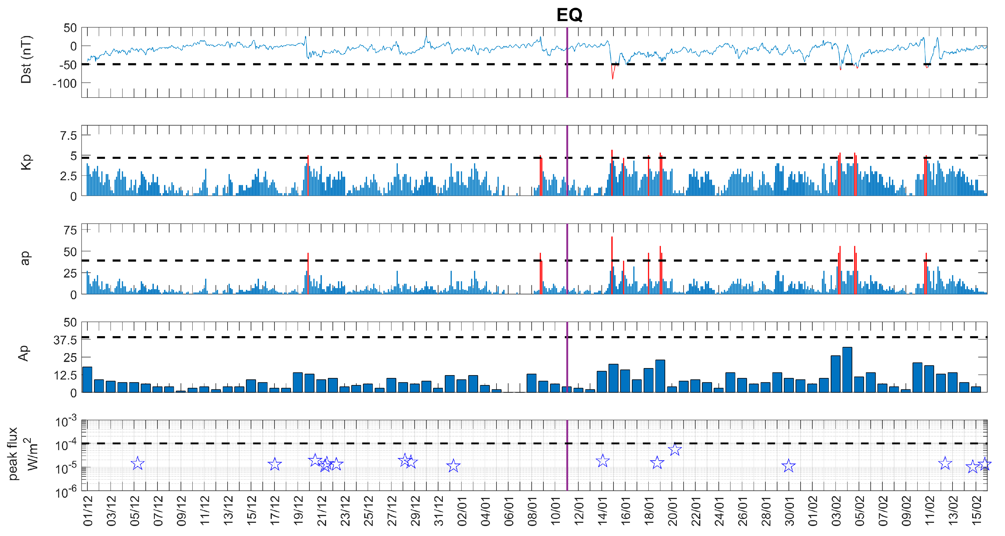
4. Analysis of the Lower Ionosphere Prior to “2021 Crete EQs” and “2022 Cyprus EQ”

In this section we present the analysis results for the three VLF/LF receivers (UWA, GER, and ACH) using the different methods and techniques presented in Section 3. Specifically, in Section 4.1 we present the results obtained with NFM, while in Section 4.2 we give the results of sequential plots of the variation of filtered signals of amplitude data and we also present the TTM results. In Section 4.3 we show the results of the NT analysis method. Finally, the results of the two techniques of wavelet analysis and LWPC are shown in Section 4.4 and Section 4.5, respectively.

4.1. NFM Analysis Results

This section analytically presents the results of the nighttime fluctuation method (NFM) by analyzing the data from the three VLF/LF stations installed in the prefecture of Attica in Athens (Greece). In the two cases of EQs under study (see Section 2), we choose the nighttime interval 21:00–02:00 UT for each baseline (between the transmitter ISR and each receiver). It is important to note that the specific nighttime interval comprises two parts, namely, one part belonging to the previous day (date) and one to the next day. In this particular application of NFM, we attribute each daily value of each statistical parameter to the next day because its (local) nighttime part is significantly larger than that of the previous day.
For the 2021 Crete EQs, we choose the period from 2 September 2021 to 29 October 2021, including at least a range of 15 days before each studied EQ’s occurrence date (see Table 1), which is appropriate for searching for EQ-related anomalies. For the 2022 Cyprus EQ, we selected the period from 2 December 2021 to 29 January 2022 for UWA and GER, while for the ACH station, due to a lack of data in November (because of some experimental setup optimizations and later on due to damage to part of the equipment by lightning), the analyzed period is from 18 December 2021 to 29 January 2022. It should be mentioned at this point that in our analysis, we have excluded any kind of artificial excerpts from the daily amplitude recordings by keeping only the natural fluctuations.
In Figure 4, we present an example of the NFM analysis results, using the GER station data, for the study of the 2022 Cyprus EQ. As we can see from Figure 4, a possible EQ-related anomaly appeared in T R * on 5 January 2022, while a simultaneous increase in N F * is also presented on the same date. In D P * , one anomaly appeared on 4 January 2022, while the other (on 11 December 2021) appeared outside of 15 days and seems unrelated to the EQ. It may be associated with two other EQ events ( Μ L 5.5 ) on 26 December 2021 and 29 December 2021 close to Crete Island (see Section 2). However, as we can see from Figure 4, an anomaly on 2 December 2021 not related to the EQ is simultaneously observed in the three statistical parameters. This anomaly is not likely to be related to the EQ under study or the EQs mentioned above due to the considerable time distance, which exceeds the range of 15 days. Therefore, it cannot be attributed to any possibly ionosphere-influencing terrestrial or extraterrestrial extreme event.
In Table 2, we present the results of the NFM analysis for the 2022 Cyprus EQ. Specifically, we present the anomalous data alongside any existing anomaly in the three VLF propagation quantities ( T R * , D P * , and N F * ) by indicating at which of the three stations (UWA, GER, and ACH) this was observed. The last column shows the attribution of each anomaly to the examined EQ, as well as to any other possibly ionosphere-influencing extreme event. The anomalies that appeared on 2 December 2021 and 27 January 2022 (see Table 2) are not attributed to any extreme event. As already mentioned, the first one appears more than 15 days before the 2022 Cyprus EQ, while the second was not followed by any extreme event.
Similar to Table 2, in Table 3 we present the UWA and GER stations’ results for the 2021 Crete EQs. All information on anomalies observed in the ISR–GER sub-ionospheric propagation path were taken from [2]. The general picture drawn by Table 3 is that anomalies associated with EQs are observed at different dates within 15 days before each EQ under study.

4.2. Diurnal Variation and TTM Analysis Results

This section presents the sequential plots of the diurnal variation of the amplitude of the filtered (by a Gaussian filter) signal, with TTs noted, as well as the results of the TTM analysis. In this study, we used the three stations to find evidence of TT shifts before each EQ under study (see Section 2). Before TT detection, we resampled the data of the UWA station to 30 s (before the filtration), so as to obtain the same sampling rate as the two other stations (see Section 2). This down-sampling of the UWA data helped us to detect the position of TT minima in parallel for all three stations. After detecting TT shifts from the sequential plots, TTM was applied, as described in Section 3.2.
In Figure 5, we give an example of the diurnal variation in sequential plots for the 2022 Cyprus EQ. In this figure, the diurnal variation of the amplitude is presented in the form of stacked 24 h signals, shifted by 10 dB. The date corresponding to each stacked signal appears in the middle (above the signal), while the selected period of this figure is from 27 December 2021 to 14 January 2022, including 15 days before the 2022 Cyprus EQ. Moreover, in Figure 5, it can be observed that two sets of TTs appear on the morning side (purple and brown circles), while on the evening side (green circles), there is only one set of TTs. In this study, we show TTs shifted towards night (see Section 2). Specifically, in the morning TTs, the brown minima appeared largely shifted (see black ellipses) towards the night on 1, 2, 8 and 9 January 2022, preceding the date of the EQ (red color). On the other hand, pre-seismic shifts are also indicated in the evening TT, which are marked as black ellipses. More specifically, significant shifts in the evening TT minima have been observed on 28 December 2021 and 9 January 2022, while a gradual shift of TTs appeared to have existed from 2 January 2022 to 6 January 2022.
The overall results of the 2022 Cyprus EQ by observing shifts of TTs for each station (UWA, ACH, and GER) are presented in Table 4. Specifically, this table gives the date of the appearance of the anomaly in UT, as well as the extreme events possibly associated with the observed anomalies. We mentioned that the chosen time for all the stations is the same as for the GER–ISR sub-ionospheric propagation path. In Table 4, we indicate each shift of TTs with the call name(s) of the stations where this is observed. TTs are referred to on the morning side as t m 1 and t m 2 , and for the evening side, as t e . The t m 1 and t e are the first selected sets of TTs towards night, while t m 2 is the second set chosen. It can be observed that most of the shifts of TTs appeared simultaneously for all stations on various dates before the EQ by considering a searching range of 15 days to find a related anomaly. Furthermore, we mention that the gradual shift of TTs, shown in Figure 5, has also very clearly been observed in the ACH station from 2 January 2022 to 6 January 2022, while in the UWA station some indications of shifts have been found on the specific dates. Yet, from Table 4, it is also noted that only one anomaly on 28 December 2021, found in t e , is possibly attributed to an EQ that occurred close to Crete Island on 29 December 2021 (see Section 2).
Similarly, by studying the 2021 Crete EQs, in Table 5, we present the summary results of the shifts of TTs detected from diurnal variation sequential plots, taking data from the UWA and GER stations. In this table there are four TT sets, two on the morning side and two on the evening side, denoted as t m 1 , t m 2 , t e 1 , and t e 2 , respectively. Again, we searched for shifts of TTs 15 days before each EQ under study. As we can see, anomalies recorded by two stations (UWA and GER) have appeared on various dates within a time range of 15 days before each EQ under study. However, we do not have data from the ACH station for September and October of 2021, as has been mentioned in Section 2, so there are no results for this station included in Table 5.
In this work, we have also applied the TTM analysis to show which pre-seismic anomalies have adequately been shifted (morning or evening TT) for each day by exceeding the threshold of ± 2 σ . More specifically, we have found the shifted TTs towards nighttime by finding the amount of shift. The procedure that has been followed is described in Section 3.2. In Figure 6, we give an example of TTM analysis for the 2022 Cyprus EQ. We have found significant shifts of TTs, which exceed the 2 σ criterion, searching for anomalies in the same studied period (2 December 2021–29 January 2022), as in the case of the NFM analysis. For the first set of TTs on the morning side towards the day, we calculated the difference of the set of TTs from the running mean window by constructing the d t m 1 time series (see Section 3.2). The same procedure (see Section 3.2) was applied for the other TT sets by calculating d t m 2 and d t e , as well as the d D V L F 1 1 time series (shift of “VLF daylength”). We note that the symbolization of d D V L F 1 1 (the same holds for each kind of shifted “VLF daylength”, e.g., d D V L F 2 1 ) shows first (reading towards right) the number of sets of TTs that are on the evening side, while the second number indicates the set of TTs that are on the morning side. As we can see, one decrement on 8 January 2022 is observed in the first panel of Figure 6, which is symbolized as d t m 1 by exceeding (shifted by −40.6 min) the threshold of 2 σ of the whole studied period (2 December 2021–29 January 2021). In the second panel for d t m 2 a shift not related to the EQ anomaly (shifted by −12.2 min) appeared on 8 December 2021. Moreover, in the third panel for d t e , only one anomalous (shifted by 26.9 min) day on 28 December 2021 existed, while in the fourth panel, presenting D V L F 1 1 , one increment (shifted by 53.9 min) on 9 January 2022 has been observed.
In Table 6, we present the overall results of the TTM analysis for the 2022 Cyprus EQ for each of the three stations (UWA, GER, and ACH). This table explicitly shows the date of the anomaly in UT and attributes any observed anomaly (shift) to the 2022 Cyprus EQ or any other possibly ionosphere-influencing extreme event. The anomalies at each shown date are denoted alongside the receiver’s call name. It is noted that the selected period for TTM analysis has been chosen similarly to the study of NFM for each station (see Section 4.1). It is evident from Table 6 that pre-seismic indications have been observed from three stations on different dates before the EQ by searching over 15 days. We note that most of these anomalies (anomalous shifts) were identified for the UWA station. It is important to note that one anomalous shift by exceeding the 2 σ in D V L F 1 1 is observed on 21 December 2021, prior to two EQs that occurred close to Crete Island (see Section 2). Moreover, anomalous dates (shifts), unlikely to be related to the 2022 Cyprus EQ, were found before (7 December 2021), as well as after (24 January 2021), its occurrence (see Table 6). The first anomalous day, before the occurrence of the EQ, is too far from the examined EQ occurrence, while the second anomalous day, after the occurrence of the 2022 Cyprus EQ, cannot be attributed to any other possibly ionosphere-influencing event.
Similarly, for the 2021 Crete EQs we present the summarized results obtained from the TTM analysis in Table 7. We used the time interval from 2 September 2021 to 29 October 2021, as in the corresponding NFM analysis (see Section 4.1). In this table, we present the shifts found on different dates before each EQ of the 2021 Crete EQs group, searching for possible pre-seismic indications 15 days before each one of them. However, we include all the detected anomalies (shifts) appearing in the studied time interval from 2 September 2021 to 29 October 2021. Thus, on only one date on 4 September 2021, we have observed anomalies (shifts) (see Table 7) from UWA station that exceed the 15 days. Finally, it is profound from Table 7 that most anomalous days come from the UWA station.

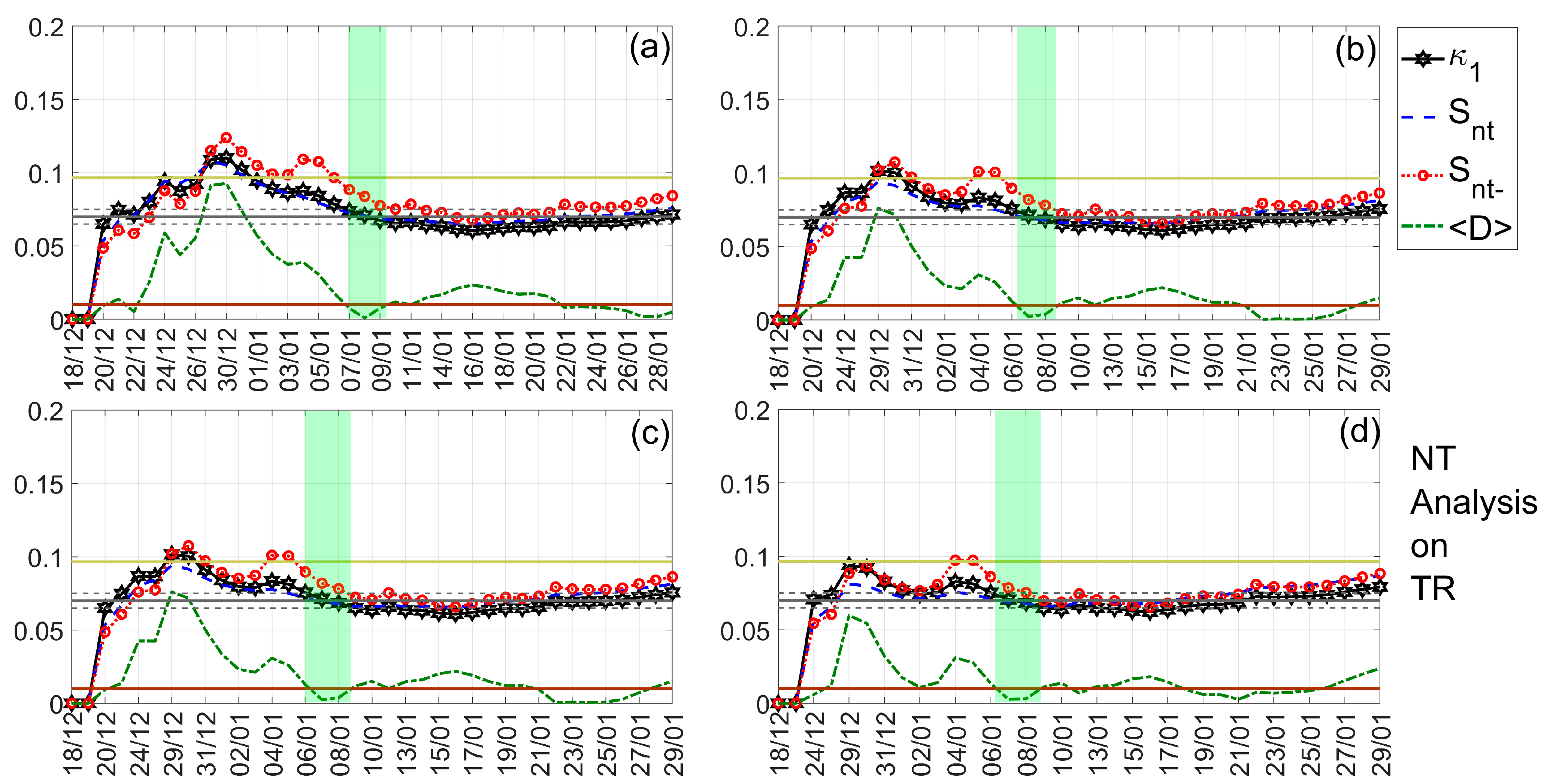
4.3. NT Analysis Results

In this section, we present the results obtained by applying the NT analysis method (see Section 3.3) to the non-normalized VLF/LF propagation quantities ( T R , D P ,   a n d   N F ) time series. We applied the NT analysis method to these non-normalized statistical quantities, as first presented for the 2020 Samos EQ and 2016 Kumamoto EQs [8,15]. The procedure to apply the NT analysis in VLF sub-ionospheric data is the same as in the case of the seismicity time series (see Section 3.3). Specifically, we consider all of the daily values of the VLF/LF propagation quantity under analysis that are higher than a certain threshold to be the “events” considered during the NT analysis, while for the k-th event Q k is considered to be equal to its corresponding daily value.
In this research, we are looking for criticality signatures that are associated with the EQ in the three statistical quantities ( T R , D P , and N F ) by presenting the results of the NT analysis method for the three stations (UWA, GER, and ACH), taking only data received by the transmitter ISR. Figure 7 presents an example of NT analysis (applied on the T R VLF propagation quantity) for the ISR–ACH sub-ionospheric propagation path prior to the 2022 Cyprus EQ. The analyzed period is from 18 December 2021 to 29 January 2022, as in the corresponding NFM analysis (see Section 4.1). The criticality conditions of NT analysis are satisfied for four thresholds, as presented in the (four) corresponding panels of Figure 7. As we can observe from this figure, criticality has been reached on 8 January 2022, which is very close in time to the examined EQ. In general, the specific criticality indication could have been considered as contaminated by a moderate geomagnetic storm (min Dst –91 nT) that happened on 14 January 2022 (see Figure 3). Yet, if one accounts for the magnitude of the EQ under study, the detected criticality is most probably reflecting the preparation of the 2022 Cyprus EQ than that of the aforementioned moderate geomagnetic storm, let alone all other less-important geomagnetic storms that happened up to ~15 days after the criticality date (see Figure 3). Finally, since only nighttime data have been used, the detected criticality has nothing to do with the preparation of any solar flare.
At this point, we should mention that criticality indications were also found after the date of the 2022 Cyprus EQ in the data acquired from all three receivers. The source of these criticality indications is not so clear, since these could be attributed either to post-EQ power laws due to “locally surviving” critical dynamics, despite the unstable critical point no longer existing, as explained in detail in [8], or to some geomagnetic events that continued up to the first days of February 2022, even though these were not that intense (see Figure 3).
In Table 8, we summarize all our findings obtained with the NT analysis in studying the 2022 Cyprus EQ. In this table, we have included all criticality signatures found by analysis of the three above-mentioned VLF/LF propagation quantities. Specifically, Table 8 indicates for each analyzed VLF/LF propagation quantity, at which receiver(s) and for which date a criticality signature has been identified, as well as the ionosphere-influencing extreme event(s) possibly related to each critical signature. As we can see from Table 8, critical signatures have been found for all three stations. We have marked each critical signature using the call name of the receiver (UWA, GER, or ACH). We should note at this point that the time range used for the NT analysis of the stations UWA and GER has been changed compared to the corresponding period used for NFM analysis (see Section 4.1). Specifically, we chose the shorter time period from 18 December 2021 to 29 January 2022 that was used during the NFM analysis of ACH. This was chosen because if one uses the wider time period (2 December 2021–29 December 2021), the NT analysis does not indicate clear criticality signatures, probably due to a masking phenomenon owing to the two EQ events that happened near Crete Island on 26 and 29 December 2021 (see Section 2). Generally, from Table 8 it can be seen that criticality signatures appear on different dates before the 2022 Cyprus EQ within 15 days prior to the EQ occurrence.
Similar to the 2022 Cyprus EQ, in Table 9, we present the results of the NT analysis for the 2021 Crete EQs. Specifically, we analyzed the VLF propagation quantities (see Section 3.1) from the UWA and GER stations by keeping the same time period that we used in the analysis of NFM. Criticality indications that appeared on different dates have been found only before the first 2021 Crete EQ within 15 days before its occurrence. A minor (min Dst = −64 nT) geomagnetic storm that occurred on 17 September 2022 21:00 (UT) is not likely to have influenced the results if one accounts for the magnitude of the first 2021 Crete EQ.

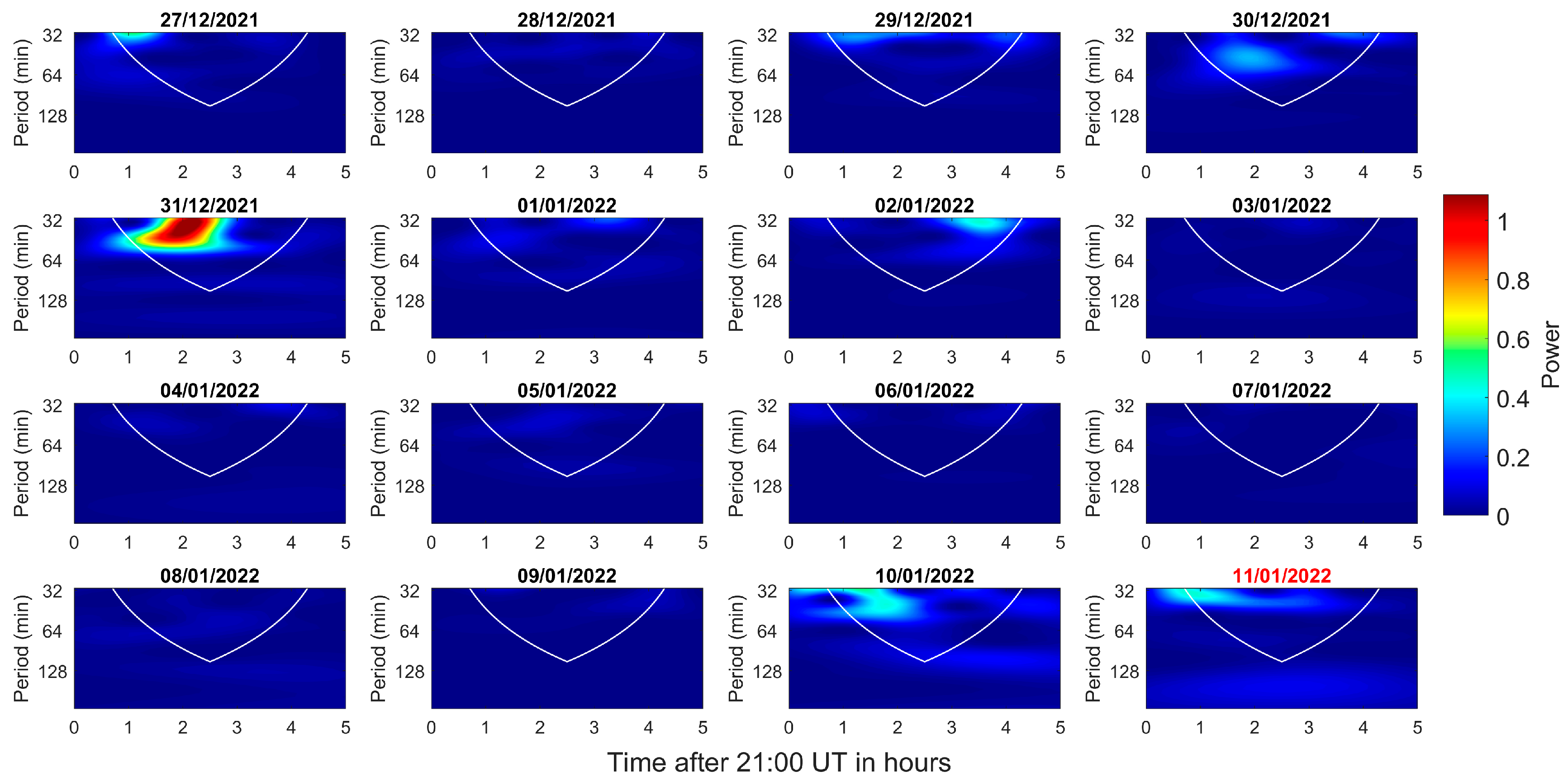
4.4. Wavelet Analysis Results

Following the procedure of applying the wavelet analysis in sub-ionospheric propagation data as described in Section 3.4, here we present the analysis results for the 2021 Crete EQs and the 2022 Cyprus EQ (see Section 3.1). In this analysis, we compute the WPS of the nighttime amplitude recordings by taking recorded data by the three stations (UWA, GER, and ACH). Specifically, we chose the same nighttime interval (21:00–02:00 UT) as we have already used in the NFM analysis (see Section 4.1). For determining the date of each WPS with the selected nighttime interval, we follow the same reasoning as in NFM (see Section 4.1).
In Figure 8, we give an example of analysis for the 2022 Cyprus EQ using the UWA receiver’s recordings. Each panel of this figure clearly shows the WPS of VLF nighttime amplitude recordings for each day, covering a period of 16 days (16 panels). Considering this figure, one significant anomaly correlated with pre-seismic AGW activity has been found 11 days (on 31 December 2021) before the EQ (the date marked at the top of the panel is colored as red). This observed enhancement in the power of WPS was found to have a periodicity of 31 to 54 min and lies within the CoI. However, more wave-like structures of intermediate intensity (and within the CoI) were observed at different dates (27 December 2021, 2, 10 and 11 January 2022), which are also possibly related to the EQ.
All the wavelet analysis findings for 2022 Cyprus EQ are summarized in Table 10, including all the results from the three stations (UWA, GER, and ACH). This table, specifically, includes the date and time of the occurrence of the AGW anomaly, its range of periodic structures, and its intensity. Furthermore, this table shows the attribution of any detected AGW anomaly to possibly ionosphere-influencing extreme event(s). However, from Table 10 we can observe only the AGW anomalies that appeared before the 2022 Cyprus EQ at dates where no other possibly ionosphere-influencing extreme event occurred, except from one case for which the anomaly could be due to another EQ of 5.7 M L that occurred on 29 December 2021 close to Crete Island.
Finally, in Table 11, we show the results of the wavelet analysis for the 2021 Crete EQs, in a form similar to the form of Table 10. Again, it can be observed that many AGW anomalies have been detected on different dates before each one of the EQs under study. However, none of these AGW anomalies are related to any other possibly ionosphere-influencing extreme event.

4.5. Simulation Results form Long Wavelength Propagation Capability Code

We present the simulation results in two parts. As mentioned above, we have focused on the morning and evening terminator times for the simulation. Therefore, we first apply the different sets around the SRT and SST to obtain the simulated amplitude value at the time of the terminators. In previous reports, e.g., [17], the simulation has been conducted to check for the entire period of sunrise and sunset times and a comparison has been presented. After that, the primary computation is associated with the perturbed ED profile during the TTs.
We used the different sets of h and β , as mentioned in Section 3.5, for the entire periods of observation in Equation (4) to obtain the altitude profile of ED. Figure 9, Figure 10 and Figure 11 show the altitude profile of ionospheric ED at SRT1, SST1, and SST2, respectively, for the ISR–UWA path in respect to the 2021 Crete EQs. The “QD” is a quiet day without EQ or space weather events. It is evident from Figure 9 that the ED decreases due to the presence of an EQ. The amount of changes in the ED profiles is not fixed. For the first 2021 Crete EQ on 27 September 2021, a moderate shift is observed on 24, 25 and 27 September 2021. It is noted that the ED profile tends to decrease before the EQ, and after the EQ, it goes in the opposite direction, leading to the quiet condition of QD. These findings corroborate the previous results when a perturbed ED usually tries to acquire its normal state (see the Introduction section). For the third 2021 Crete EQ on 19 October 2021, the changes in the ED are more significant, and the maximum decrease in ED is observed on 16 October 2021, 17 October 2021, and also on the EQ day on 19 October 2021. Therefore, both pre- and co-seismic effects are present in this case.
Figure 10 and Figure 11 present similar ED profiles for SST1 and SST2 for the ISR–UWA path. For the sunset times, we examine both the sunset terminators. In contrast to the SRT, for SST1, we found significantly perturbed ED profiles only for the second 2021 Crete EQ on 12 October 2021. The maximum shifts in ED take place on 11 October 2021 and 12 October 2021. It is evident that the ED profile for SST1 returns to its original values after the EQ on 12 October 2021, and no further significant changes have been observed. For the SST2, the changes in the ED are random with no such prominent decreasing nature.
The variation of ED for the ISR–GER path with respect to the 2021 Crete EQs is shown in Figure 12, Figure 13 and Figure 14. For the ISR–GER path, we examine one SRT (SRT1) and two SSTs (SST1 and SST2), as for the UWA signal. For the 27 September 2021 EQ, no changes in ED have been observed. However, for the EQ on 12 October 2021, significant changes in the ED profile are observed on 11 October 2021 from its typical values, while for the 19 October 2021 EQ, a greater decrement in ED is observed on the day of the EQ.
In the case of SSTs, it is evident from Figure 13 that the ED profiles are a bit random for this terminator. For the EQ on 27 September 2021, the values of ED at SST1 are found to be unperturbed both on the EQ day and prior to the same. This is consistent with the ISR path ED profile during SST, where we failed to observe any significant changes in ED. However, for the EQs on 12 October 2021 and 19 October 2021, substantial changes in the ED profile are observed. For the 12 October 2021 EQ, the maximum changes in ED are observed on the day of the EQ, followed by intermediate changes on 11 October 2021. Similarly, for the 19 October 2021 EQ, significant changes in ED are found on the day of the EQ, followed by intermediate changes on 14 October 2021.
For the SST2 variation, we observed only significant changes for the EQ on 27 September 2021. However, we observed the change long back on 13 September 2021 and 15 September 2021. This is a bit unusual compared to the other ED profiles for which we found the changes in ED within a shorter period of time before the EQ. It is also evident from Figure 13 that there are examples of enhancement of ED in the intermediate periods of those EQs. This effect can be attributed to three consecutive EQs during the observation period. We also observed the shift in TT in opposite directions. Therefore, the modal conversion of the waves possibly behaves oppositely. It is well-established that during the SRTs and SSTs, a conventional waveguide mode conversion occurs due to variation in the ED profiles due to solar irradiance. As the seismogenic perturbation is not controlled but random both ways, TT shifts have been observed in many previous cases, but it is to be noted that the perturbation in ED primarily decreases consistently during or before the EQ.
The similar variation of the altitude profiles of ED at SRT and SST for the ISR–UWA path during the 2022 Cyprus EQ on 11 January 2022 is shown in Figure 15 and Figure 16, respectively. It is evident from Figure 15 that a considerable amount of decrement of ED is observed on the day of the EQ (11 January 2022), and intermediate decrease in EDs from the quiet day ED profiles (QD) are observed on 1, 8 and 9 January 2022. For the SST, a similar decrement in the ED profiles has been observed before the EQ day (on 5, 6, 7 and 9 January 2022), while for the day of the EQ, the ED profiles slightly increased. This is quite an exciting result where the co-seismic effect is somewhat opposite to the pre-seismic variation.

4.6. Summary of Analysis Results

By taking into account all the results presented in the previous ubsections of Section 4, in this Subsection we summarize the main findings of the whole research:
Within 15 days before each studied EQ (2022 Cyprus EQ and 2021 Crete EQs), anomalies and criticality signatures have been revealed for different days from all the analysis methods and techniques (see Table 2, Table 3, Table 4, Table 5, Table 6, Table 7, Table 8, Table 9, Table 10 and Table 11). It is noted that any possible influence on the presented results from ionosphere-influencing extreme events (e.g., solar flares, geomagnetic storms, EQs, volcanoes), other than the EQs under study have been discussed in detail, whereas any possible attribution of the revealed anomalies and criticality signatures to them has been included in Table 2, Table 3, Table 4, Table 5, Table 6, Table 7, Table 8, Table 9, Table 10 and Table 11.
By analyzing with NFM, taking data from the three sub-ionospheric propagation paths (ISR–UWA, ISR–GER, ISR–ACH) with respect to the 2022 Cyprus EQ, we can observe several VLF anomalies exceeding the +2 σ /−2 σ limits (see Table 2). These are found in all the sub-ionospheric propagation paths in the three VLF propagation quantities. However, two other EQ events (occurred on 26 December 2021 and 29 December 2021, respectively) that also occurred in the southeastern Mediterranean, not the focus of this study, are found to be correlated with only two anomalous days on 11 December 2021 and 21 December 2021 (see Table 2). Moreover, it is also found that two anomalous days (2 December 2021 and 27 December 2021) are not associated with any possibly ionosphere-influencing extreme event. Similar to the 2022 Cyprus EQ case, there are VLF anomalies attributed to the three 2021 Crete EQs in the three VLF propagation quantities (exceeding the +2 σ /−2 σ limits) for the two sub-ionospheric propagation paths for which adequate data were available (ISR–UWA and ISR–GER) (Table 3). In this case, no other extreme event occurred around the studied time period. However, two detected anomalous days (5 September 2021 and 27 October 2021) in Table 3 are not attributed to any known possibly ionosphere-influencing extreme event.
From the sequential plots of the diurnal variation of the received amplitude in regard to the 2022 Cyprus EQ, we have observed pre-EQ shifts of TT minima towards the nighttime in all studied sub-ionospheric propagation paths (ISR–UWA, ISR–GER, ISR–ACH) for two out of the three TTs ( t m 1 and t e ) (Table 4). For the third TT ( t m 2 ) there is no observed shift. Moreover, one of the two EQs not the focus of this study (mentioned above) is found to be possibly related to one shifted day (28 December 2021). In a more detailed analysis, by applying the TTM (see Table 6), it is evident that shifts (also noting the amount of shift) of TTs exceeding ± 2 σ are found in all three paths for the three TT sets ( t m 1 , t m 2 , and t e ). However, three observed anomalous shifts, detected earlier and later than the EQ on 7 December 2021, 8 December 2021, and 24 January 2021, are not linked with any extreme event. Yet, the two aforementioned EQs that are not the focus of this study are likely to be associated with two anomalous days with 21 December 2021, while one of them is associated with 28 December 2021, by pointing out that their occurrence is closer in time to these observed anomalies, in contrast to the examined EQ. From the sequential plots of the diurnal variation of the received amplitude in regard to the 2021 Crete EQs (see Table 5), we found pre-EQ shifts of TT minima towards nighttime in four TT sets ( t m 1 , t m 2 , t e 1 , and t e 2 ) by observing shifts of TT minima for the paths ISR–UWA and ISR–GER. On the other hand, using the TTM, shifts were also detected for both paths (Table 7), while only one shifted day on 4 September 2021 is not associated with an EQ.
By applying the NT analysis on non-normalized VLF propagation quantities in the case of 2022 Cyprus EQ, it is found that the criticality signatures are detected at different dates before and after the EQ for all three propagation paths (ISR–UWA, ISR–GER, ISR–ACH) (see Table 8). More specifically, the criticality signatures that appeared before the EQ can be attributed to the specific seismic event under study, while the source of the criticality indications found after the 2022 Cyprus EQ (during the time period 15 January 2022–25 January 2022) is not so clear. These could be attributed either to post-EQ power laws [8] due to “locally surviving” critical dynamics, despite the unstable critical point no longer existing, or to some geomagnetic events, even though these were not very intense. In the case of applying the NT analysis method to the non-normalized VLF propagation quantities for the 2021 Crete EQs, criticality has been detected in both paths for which adequate data were available (ISR–UWA and ISR–GER), but only for the first EQ that occurred on 27 September 2021 (see Table 9).
Regarding the wavelet analysis (see Table 10) of VLF data for the 2022 Cyprus EQ, it is found that AGW-related anomalies existed in all three propagation paths on different days before the studied EQ. High- and moderate-intensity patches of wave-like structures are generally unveiled in a range of ~30–60 min, with varying time intervals. At this point, it needs to be mentioned that only one AGW-related anomaly is associated with the EQ that occurred in the southeastern Mediterranean on 27 December 2021 that was not the focus of this study as presented in Table 10. Similarly, by analyzing the VLF data for the 2021 Crete EQs, AGW activity appeared at different dates before each studied EQ in the propagation paths ISR–UWA and ISR–GER. The detected high- and moderate-intensity patches of wave-like structures appeared, most of them from ~30–60 min, while very few exceed the periodicity of ~60 min. It is finally mentioned that no other possibly ionosphere-influencing extreme event is associated with these observed AGW anomalies.
The LWPC simulation of perturbed ED finds significant variation during the SRT and SST times for the four EQs that are the focus of this study. In Figure 9, Figure 10, Figure 11, Figure 12, Figure 13, Figure 14, Figure 15 and Figure 16, it is evident that, for all the EQs, the electron density becomes mostly depleted. Moreover, it needs to be mentioned that we have observed both pre- and co-seismic perturbation of ED profiles for these EQs. The changes vary from roughly 0.5 × 10 9   t o   3 × 10 9 / m 3 . Some exciting features are found in this analysis. The ED profiles during SRT seem more prominently perturbed compared to the SST. For the Crete EQs, not all the paths show identical ED profiles for SRT and SSTs. The usual ED perturbation for SRT lies within 0 to 7 days before the EQs (Figure 9, Figure 10, Figure 12 and Figure 13). On the other hand, during the SST2, the UWA signal does not have any effect, while for the GER signal, SST2 shows a variation quite a long time (14 days) before the EQ (Figure 11 and Figure 14). However, for the 2022 Cyprus EQ, the ED variation shows an anomalous decrement for both the SRT and SST period. We anticipate this inhomogeneity due to different modal interference processes at different stations.

5. Conclusions

This paper elaborately presented the analysis of VLF/LF sub-ionospheric propagation data from one VLF transmitter (with call name ISR and operation at 29.7 kHz). At the same time, their acquisition was performed by three VLF/LF receivers located in Athens (Greece). In this attempt, we used several analysis methods in order to detect pre-seismic indications in a time range of 15 days before the 2021 Crete EQs and the 2022 Cyprus EQ. This aim was indeed achieved, confirming previous studies
On the other hand, except the EQs in the focus of this study, several other possibly ionosphere-influencing extreme events have been found close within a relatively short time distance (within 15 days) from the revealed anomalies and criticality indications. For this reason, we attributed any possible candidate extreme event to any of each possible aforementioned anomaly/criticality indication.
Moreover, it was found that, in some cases, the identified anomalies or criticality signatures were revealed after the occurrence of an EQ. This could be due to other possible ionosphere-influencing extreme events that occurred within a relatively short time distance (~15 days) after the detected anomalies or criticality signatures, or, for the case of criticality indications, to possible post-EQ power laws due to “locally surviving” critical dynamics, despite the unstable critical point no longer existing [8].
Moreover, by applying the LWPC simulation for TT minima, using data from the three VLF/LF stations, we found perturbations (increases or decreases) of ED for all the studied EQs. Past studies, e.g., [17,25,37], which similarly showed ED perturbations on shifted TTs, are in agreement with the findings of the present work.
To sum up, this paper clearly shows that the lower ionosphere appears to carry a pre-seismic imprint before the occurrence of each studied EQ, using various analysis methods. However, more research efforts are needed in the future in order to find more evidence to attribute an anomaly to a specific extreme event by taking a further step towards understanding the nature of the phenomena preceding an impending EQ.

Author Contributions

Conceptualization, S.M.P., S.S. and M.H.; methodology, D.Z.P., S.M.P., S.S. and M.H.; software, D.Z.P., S.M.P. and S.S.; validation, D.Z.P., S.M.P., S.S, F.M., D.D. and M.H.; formal analysis, D.Z.P. and S.S.; investigation, D.Z.P., S.M.P. and S.S.; resources, D.Z.P., S.M.P., F.M., D.D. and M.H.; visualization, D.Z.P., S.M.P. and S.S; writing—original draft preparation, D.Z.P., S.M.P. and S.S.; writing—review and editing, D.Z.P., S.M.P., S.S, F.M., D.D. and M.H.; supervision, S.M.P. All authors have read and agreed to the published version of the manuscript.

Funding

This research received no external funding.

Data Availability Statement

The VLF/LF data presented in this study are available on request from the corresponding author. All other data are publicly available from the sources mentioned in the manuscript.

Acknowledgments

The authors would like to express their gratitude to the Institute of Geodynamics of the National Observatory of Athens for the seismic catalogs; to the World Data Center for Geomagnetism of Kyoto for the geomagnetic indices Dst, Kp, ap, and Ap data; to the USA National Oceanic and Atmospheric Administration for the solar X-ray flux data; to the Global Volcanism Program of the Smithsonian Institution for the volcano eruption data; to the Ventusky search engine, the USA National Oceanic and Atmospheric Administration (NOAA), and the Deutscher Wetter-dienst (DWD) for the CAPE parameter data; as well as to Blitzortung.org and lightningmaps.org for the lightning activity data.

Conflicts of Interest

The authors declare no conflict of interest.

References

  1. Hayakawa, M. Probing the lower ionospheric perturbations associated with earthquakes by means of subionospheric VLF/LF propagation. Earthq. Sci. 2011, 24, 609–637. [Google Scholar] [CrossRef]
  2. Malkotsis, F.; Politis, D.Z.; Dimakos, D.; Potirakis, S.M. An amateur-radio-based open-source (HW/SW) VLF/LF receiver for lower ionosphere monitoring, examples of identified perturbations. Foundations 2022, 2, 639–663. [Google Scholar] [CrossRef]
  3. Rozhnoi, A.; Hayakawa, M.; Solovieva, M.; Hobara, Y.; Fedun, V. Ionospheric effects of the Mt. Kirishima volcanic eruption as seen from Subionospheric VLF Observations. J. Atmos. Sol. Terr. Phys. 2014, 107, 54–59. [Google Scholar] [CrossRef]
  4. Rodger, C.J. Subionospheric VLF perturbations associated with lightning discharges. J. Atmos. Sol. Terr. Phys. 2003, 65, 591–606. [Google Scholar] [CrossRef]
  5. Biagi, P.F.; Maggipinto, T.; Righetti, F.; Loiacono, D.; Schiavulli, L.; Ligonzo, T.; Ermini, A.; Moldovan, I.A.; Moldovan, A.S.; Buyuksarac, A.; et al. The European VLF/LF Radio Network to search for earthquake precursors: Setting up and natural/man-made disturbances. Nat. Hazards Earth Syst. Sci. 2011, 11, 333–341. [Google Scholar] [CrossRef]
  6. Chakrabarti, S.K.; Mondal, S.K.; Sasmal, S.; Pal, S.; Basak, T.; Chakrabarti, S.; Bhowmick, D.; Ray, S.; Maji, S.K.; Nandi, A.; et al. VLF signals in summer and winter in the Indian sub-continent using multi-station campaigns. Indian J. Phys. 2012, 86, 323–334. [Google Scholar] [CrossRef]
  7. Raulin, J.-P.; Bertoni, F.C.; Gavilán, H.R.; Guevara-Day, W.; Rodriguez, R.; Fernandez, G.; Correia, E.; Kaufmann, P.; Pacini, A.; Stekel, T.R.; et al. Solar flare detection sensitivity using the South America VLF Network (SAVNET). J. Geophys. Res. Space Phys. 2010, 115, A7. [Google Scholar] [CrossRef]
  8. Politis, D.Z.; Potirakis, S.M.; Contoyiannis, Y.F.; Biswas, S.; Sasmal, S.; Hayakawa, M. Statistical and criticality analysis of the lower ionosphere prior to the 30 October 2020 Samos (Greece) earthquake (M6.9), based on VLF electromagnetic propagation data as recorded by a new VLF/LF receiver installed in Athens (Greece). Entropy 2021, 23, 676. [Google Scholar] [CrossRef] [PubMed]
  9. Freund, F.T.; Kulahci, I.G.; Cyr, G.; Ling, J.; Winnick, M.; Tregloan-Reed, J.; Freund, M.M. Air ionization at rock surfaces and pre-earthquake signals. J. Atmos. Sol.-Terr. Phys. 2009, 71, 1824–1834. [Google Scholar] [CrossRef]
  10. Eftaxias, K.; Potirakis, S.M.; Contoyiannis, Y. 13-Four-stage model of earthquake generation in terms of fracture-induced electromagnetic emissions. In Complexity of Seismic Time Series, 1st ed.; Chelidze, T., Vallianatos, F., Telesca, L., Eds.; Elsevier: Amsterdam, The Netherlands, 2018; pp. 437–502. [Google Scholar] [CrossRef]
  11. Varotsos, P.A.; Sarlis, N.V.; Skordas, E.S. Natural Time Analysis: The New View of Time Precursory Seismic Electric Signals, Earthquakes and Other Complex Time Series, 1st ed.; Springer: Berlin/Heidelberg, Germany, 2011. [Google Scholar] [CrossRef]
  12. Contoyiannis, Y.; Potirakis, S.M.; Eftaxias, K.; Hayakawa, M.; Schekotov, A. Intermittent criticality revealed in ULF Magnetic Fields prior to the 11 March 2011 Tohoku earthquake (Mw = 9). Phys. A Stat. Mech. Appl. 2016, 452, 19–28. [Google Scholar] [CrossRef]
  13. Hayakawa, M.; Schekotov, A.; Potirakis, S.M.; Eftaxias, K.; Li, Q.; Asano, T. An integrated study of ULF magnetic field variations in association with the 2008 Sichuan earthquake, on the basis of statistical and critical analyses. Open J. Earthq. Res. 2015, 04, 85–93. [Google Scholar] [CrossRef]
  14. Potirakis, S.M.; Contoyiannis, Y.; Asano, T.; Hayakawa, M. Intermittency-induced criticality in the lower ionosphere prior to the 2016 Kumamoto earthquakes as embedded in the VLF propagation data observed at multiple stations. Tectonophysics 2018, 722, 422–431. [Google Scholar] [CrossRef]
  15. Potirakis, S.; Asano, T.; Hayakawa, M. Criticality analysis of the lower ionosphere perturbations prior to the 2016 Kumamoto (Japan) earthquakes as based on VLF electromagnetic wave propagation data observed at multiple stations. Entropy 2018, 20, 199. [Google Scholar] [CrossRef]
  16. Hayakawa, M.; Molchanov, O.A.; Ondoh, T.; Kawai, E. Anomalies in the sub-ionospheric VLF signals for the 1995 Hyogo-Ken Nanbu earthquake. J. Phys. Earth 1996, 44, 413–418. [Google Scholar] [CrossRef]
  17. Biswas, S.; Chowdhury, S.; Sasmal, S.; Politis, D.Z.; Potirakis, S.M.; Hayakawa, M. Numerical modelling of sub-ionospheric very low frequency radio signal anomalies during the Samos (Greece) earthquake (M = 6.9) on October 30, 2020. Adv. Space Res. 2022, 70, 1453–1471. [Google Scholar] [CrossRef]
  18. Torrence, C.; Compo, G.P. A practical guide to wavelet analysis. Bull. Am. Meteorol. Soc. 1998, 79, 61–78. [Google Scholar] [CrossRef]
  19. Biswas, S.; Kundu, S.; Ghosh, S.; Chowdhury, S.; Yang, S.-S.; Hayakawa, M.; Chakraborty, S.; Chakrabarti, S.K.; Sasmal, S. Contaminated effect of geomagnetic storms on pre-seismic atmospheric and ionospheric anomalies during Imphal earthquake. Open J. Earthq. Res. 2020, 09, 383–402. [Google Scholar] [CrossRef]
  20. Biswas, S.; Kundu, S.; Sasmal, S.; Politis, D.Z.; Potirakis, S.M.; Hayakawa, M. Preseismic perturbations and their inhomogeneity as computed from ground- and space-based investigation during the 2016 Fukushima earthquake. J. Sens. 2023, 2023, 7159204. [Google Scholar] [CrossRef]
  21. Righetti, F.; Biagi, P.F.; Maggipinto, T.; Schiavulli, L.; Ligonzo, T.; Ermini, A.; Moldovan, I.A.; Moldovan, A.S.; Buyuksarac, A.; Silva, H.G.; et al. Wavelet analysis of the LF radio signals collected by the European VLF/LF network from July 2009 to April 2011. Ann. Geophys. 2012, 55, 171–180. [Google Scholar] [CrossRef]
  22. Ferguson, J.A. Computer Programmes for Assessment of Long Wavelength Radio Communications; Version 2.0, Tech. doc. 3030; Space and Naval Warfare Systems Center: San Diego, CA, USA, 1998. [Google Scholar]
  23. Grubor, D.P.; Šulić, D.M.; Žigman, V. Classification of X-ray solar flares regarding their effects on the lower ionosphere electron density profile. Ann. Geophys. 2008, 26, 1731–1740. [Google Scholar] [CrossRef]
  24. Maurya, A.K.; Venkatesham, K.; Kumar, S.; Singh, R.; Tiwari, P.; Singh, A.K. Effects of St. Patrick’s day geomagnetic storm of March 2015 and of June 2015 on low-equatorial D region ionosphere. J. Geophys. Res. Space Phys. 2018, 123, 6836–6850. [Google Scholar] [CrossRef]
  25. Ghosh, S.; Chakraborty, S.; Sasmal, S.; Basak, T.; Chakrabarti, S.K.; Samanta, A. Comparative study of the possible lower ionospheric anomalies in very low frequency (VLF) signal during Honshu, 2011 and Nepal, 2015 earthquakes. Geomat. Nat. Hazards Risk 2019, 10, 1596–1612. [Google Scholar] [CrossRef]
  26. Cummer, S.A.; Inan, U.S.; Bell, T.F. Ionospheric D region remote sensing using VLF radio atmospherics. Radio Sci. 1998, 33, 1781–1792. [Google Scholar] [CrossRef]
  27. Wait, J.R.; Spies, K.P. Characteristics of the Earth–Ionosphere Waveguide for VLF Radio Waves; NBS Technical Note 300; US Department of Commerce, National Bureau of Standards: Washington, DC, USA, 1964. [Google Scholar]
  28. Tatsuta, K.; Hobara, Y.; Pal, S.; Balikhin, M. Sub-ionospheric VLF signal anomaly due to geomagnetic storms: A statistical study. Ann. Geophys. 2015, 33, 1457–1467. [Google Scholar] [CrossRef]
  29. Rozhnoi, A.; Solovieva, M.S.; Molchanov, O.A.; Hayakawa, M. Middle latitude LF (40 kHz) phase variations associated with earthquakes for quiet and disturbed geomagnetic conditions. Phys. Chem. Earth 2004, 29, 589–598. [Google Scholar] [CrossRef]
  30. Maekawa, S.; Horie, T.; Yamauchi, T.; Sawaya, T.; Ishikawa, M.; Hayakawa, M.; Sasaki, H. A statistical study on the effect of earthquakes on the ionosphere, based on the subionospheric LF propagation data in Japan. Ann. Geophs. 2006, 24, 2219–2225. [Google Scholar] [CrossRef]
  31. Kasahara, Y.; Muto, F.; Horie, T.; Yoshida, M.; Hayakawa, M.; Ohta, K.; Rozhnoi, A.; Solovieva, M.; Molchanov, O.A. On the statistical correlation between the ionospheric perturbations as detected by subionospheric VLF/LF propagation anomalies and earthquakes. Nat. Hazards Earth Syst. Sci. 2008, 8, 653–656. [Google Scholar] [CrossRef]
  32. Yoshida, M.; Yamauchi, T.; Horie, T.; Hayakawa, M. On the generation mechanism of terminator times in subionospheric VLF/LF propagation and its possible application to seismogenic effects. Nat. Hazards Earth Syst. Sci. 2008, 8, 129–134. [Google Scholar] [CrossRef]
  33. Molchanov, O.A.; Hayakawa, M. Subionospheric VLF signal perturbations possibly related to earthquakes. J. Geophys. Res. Space Phys. 1998, 103, 17489–17504. [Google Scholar] [CrossRef]
  34. Ray, S.; Chakrabarti, S.K. A Study of the Behavior of the Terminator Time Shifts Using Multiple VLF Propagation Paths During the Pakistan Earthquake (M = 7.2) of 18 January 2011. Nat. Hazards Earth Syst. Sci. 2013, 13, 1501–1506. [Google Scholar] [CrossRef]
  35. Sasmal, S.; Chakrabarti, S.K. Ionosperic Anomaly Due to Seismic Activities—Part 1: Calibration of the VLF Signal of VTX 18.2 Khz Station from Kolkata and Deviation During Seismic Events. Nat. Hazards Earth Syst. Sci. 2009, 9, 1403–1408. [Google Scholar] [CrossRef]
  36. Sasmal, S.; Chakrabarti, S.K.; Chakrabarti, S. Studies of the correlation between ionospheric anomalies and seismic activities in the Indian subcontinent. AIP Conf. Proc. 2010, 1286, 270. [Google Scholar] [CrossRef]
  37. Chakraborty, S.; Sasmal, S.; Basak, T.; Ghosh, S.; Palit, S.; Chakrabarti, S.K.; Ray, S. Numerical Modeling of Possible Lower Ionospheric Anomalies Associated with Nepal Earthquake in May, 2015. Adv. Space Res. 2017, 60, 1787–1796. [Google Scholar] [CrossRef]
  38. Chakrabarti, S.K.; Saha, M.; Khan, R.; Mandal, S.; Acharyya, K.; Saha, R. Possible Detection of Ionospheric Disturbances During the Sumatra-Andaman Islands Earthquakes of December, 2004. Indian J. Radio Sp. Phys. 2005, 34, 314–317. [Google Scholar]
  39. Chakrabarti, S.; Sasmal, S.; Saha, M.; Khan, R.; Bhoumik, D.; Chakrabarti, S.K. Unusual Behavior of D-Region Ionization Time at 18.2kHz During Seismically Active Days. Indian J. Phys. 2007, 81, 531–538. [Google Scholar]
  40. Chakrabarti, S.K.; Sasmal, S.; Chakrabarti, S. Ionospheric Anomaly Due to Seismic Activities—Part 2: Evidence from D-Layer Preparation and Disappearance Times. Nat. Haz. Earth Syst. Sci. 2010, 10, 1751–1757. [Google Scholar] [CrossRef]
  41. Ray, S.; Chakrabarti, S.K.; Sasmal, S.; Choudhury, A.K.; Chakrabarti, S.K. Correlations between the anomalous behavior of the ionosphere and the seismic events for VTX-MALDA VLF propagation. AIP Conf. Proc. 2010, 1286, 298. [Google Scholar] [CrossRef]
  42. Ray, S.; Chakrabarti, S.K.; Mondal, S.K.; Sasmal, S. Ionospheric Anomaly Due to Seismic Activities-III: Correlation Between Night Time VLF Amplitude Fluctuations and Effective Magnitudes of Earthquakes in Indian Sub-Continent. Nat. Hazards Earth Syst. Sci. 2011, 11, 2699–2704. [Google Scholar] [CrossRef]
  43. Ray, S.; Chakrabarti, S.K.; Sasmal, S. Precursory Effects in the Nighttime VLF Signal Amplitude for the 18th January, 2011 Pakistan Earthquake. Indian J. Phys. 2012, 86, 85–88. [Google Scholar] [CrossRef]
  44. Sasmal, S.; Chakrabarti, S.K.; Ray, S. Unusual Behavior of Very Low Frequency Signal During the Earthquake at Honshu/Japan on 11 March, 2011. Indian J. Phys. 2014, 88, 1013–1019. [Google Scholar] [CrossRef]
  45. Pal, P.; Sasmal, S.; Chakrabarti, S.K. Studies of Seismo-Ionospheric Correlations Using Anomalies in Phase of Very Low Frequency Signal. Geomat. Nat. Haz. Risk 2017, 8, 167–176. [Google Scholar] [CrossRef]
  46. Varotsos, P.A.; Sarlis, N.V.; Skordas, E.S. Long-Range Correlations in the Electric Signals that Precede Rupture. Phys. Rev. E 2002, 66, 011902. [Google Scholar] [CrossRef] [PubMed]
  47. Varotsos, P.A.; Sarlis, N.V.; Tanaka, H.K.; Skordas, E.S. Similarity of Fluctuations in Correlated Systems: The Case of Seismicity. Phys. Rev. E 2005, 72, 041103. [Google Scholar] [CrossRef]
  48. Varotsos, P.A.; Sarlis, N.V.; Skordas, E.S. Spatio-Temporal Complexity Aspects on the Interrelation Between Seismic Electric Signals and Seismicity. Pract. Athens Acad. 2001, 76, 294–321. [Google Scholar]
  49. Abe, S.; Sarlis, N.V.; Skordas, E.S.; Tanaka, H.K.; Varotsos, P.A. Origin of the Usefulness of the Natural-Time Representation of Complex Time Series. Phys. Rev. Lett. 2005, 94, 170601. [Google Scholar] [CrossRef] [PubMed]
  50. Potirakis, S.M.; Contoyiannis, Y.; Schekotov, A.; Eftaxias, K.; Hayakawa, M. Evidence of critical dynamics in various electromagnetic precursors. Eur. Phys. J. Spec. Top. 2021, 230, 151–177. [Google Scholar] [CrossRef]
  51. Ghosh, S.; Chowdhury, S.; Kundu, S.; Sasmal, S.; Politis, D.Z.; Potirakis, S.M.; Hayakawa, M.; Chakraborty, S.; Chakrabarti, S.K. Unusual surface latent heat flux variations and their critical dynamics revealed before strong earthquakes. Entropy 2021, 24, 23. [Google Scholar] [CrossRef]
  52. Yang, S.-S.; Potirakis, S.M.; Sasmal, S.; Hayakawa, M. Natural Time Analysis of global navigation satellite system surface deformation: The case of the 2016 Κumamoto earthquakes. Entropy 2020, 22, 674. [Google Scholar] [CrossRef]
  53. Politis, D.Z.; Potirakis, S.M.; Kundu, S.; Chowdhury, S.; Sasmal, S.; Hayakawa, M. Critical Dynamics in stratospheric potential energy variations prior to significant (M > 6.7) earthquakes. Symmetry 2022, 14, 1939. [Google Scholar] [CrossRef]
  54. Potirakis, S.M.; Karadimitrakis, A.; Eftaxias, K. Natural time analysis of critical phenomena: The case of pre-fracture electromagnetic emissions. Chaos 2013, 23, 023117. [Google Scholar] [CrossRef]
  55. Varotsos, P.A.; Sarlis, N.V.; Skordas, E.S.; Tanaka, H.K.; Lazaridou, M.S. Entropy of Seismic Electric Signals: Analysis in the Natural Time Under Time Reversal. Phys. Rev. E 2006, 73, 031114. [Google Scholar] [CrossRef] [PubMed]
  56. Sarlis, N.V.; Skordas, E.S.; Varotsos, P.A. Similarity of Fluctuations in Systems Exhibiting Self-Organized Criticality. Europhys. Lett. 2011, 96, 28006. [Google Scholar] [CrossRef]
  57. Sarlis, N.V.; Skordas, E.S.; Lazaridou, M.S.; Varotsos, P.A. Investigation of Seismicity After the Initiation of a Seismic Electric Signal Activity Until the Mainshock. Proc. Jpn. Acad. Ser. B 2008, 84, 331–343. [Google Scholar] [CrossRef]
  58. Sasmal, S.; Pal, S.; Chakrabarti, S.K. Study of long path VLF signal propagation characteristics as Observed from Indian Antarctic station, Maitri. Adv. Space Res. 2014, 54, 1619–1628. [Google Scholar] [CrossRef]
  59. Sasmal, S.; Palit, S.; Chakrabarti, S.K. Modeling of long path propagation characteristics of Very Low Frequency (VLF) radio waves as observed from Indian Antarctic station. J. Geophys. Res. Space Phys. 2015, 120, 8872–8883. [Google Scholar] [CrossRef]
  60. Sasmal, S.; Basak, T.; Chakraborty, S.; Palit, S.; Chakrabarti, S.K. Modeling of temporal variation of Very Low Frequency (VLF) radio waves over long paths as observed from Indian Antarctic stations. J. Geophys. Res. Space Phys. 2017, 122, 7698–7712. [Google Scholar] [CrossRef]
  61. Chowdhury, S.; Kundu, S.; Ghosh, S.; Basak, T.; Hayakawa, M.; Chakraborty, S.; Chakrabarti, S.K.; Sasmal, S. Numerical simulation of lower ionospheric reflection parameters by using International Reference Ionosphere (IRI) model and validation with Very Low Frequency (VLF) radio signal characteristics. Adv. Space Res. 2021, 67, 1599–1611. [Google Scholar] [CrossRef]
Figure 1. Satellite image of the prefecture of Attica in Greece. The three VLF/LF stations (ACH, GER, and UWA) are depicted with light green squares, while the distance between each pair of them is also shown.
Atmosphere 14 00673 g001
Figure 2. Map of the eastern Mediterranean. The 5th Fresnel zone of the propagation path between the three receivers and the transmitter ISR is indicated, whereas the epicenters of the studied EQs are shown as pentagrams and each occurrence date is shown alongside the corresponding epicenter.
Atmosphere 14 00673 g002
Figure 3. Geomagnetic indices Dst, Kp, ap, and Ap, as well as solar flares during the time period 1 December 2021–15 February 2022, which are indicated as pentagrams. Red-colored parts indicate values exceeding the thresholds marked by the horizontal black dashed lines. In the case of the bottom panel, the threshold separates M class from X class solar flares.
Atmosphere 14 00673 g003
Figure 4. Time evolution of three statistical quantities, T R * , D P * ,   a n d   N F * , of the NFM analysis method for the sub−ionospheric path GER−ISR is shown in the top, middle, and bottom panels, respectively. The time period represented in the figure is from 2 December 2021 to 29 January 2022. Red solid horizontal lines indicate the corresponding +2 σ /−2 σ limits; σ is calculated for the whole studied period of each panel. The date of EQ is shown on top of each panel by the purple vertical line segment, marked on the top of each panel.
Atmosphere 14 00673 g004
Figure 5. Diurnal variation of the amplitude of the VLF signal of the propagation path GER–ISR for the time period 27 December 2021–14 January 2022. Each signal is vertically shifted by +10 dB in regards to the signal of the previous day. Brown and purple circles indicate the minima identified as morning TTs before and after the sunrise, respectively. Green circles are the evening TTs, which appear before the sunset. Finally, the date of the EQ is marked with red color. The black circles indicate the existence of shifts of TTs.
Atmosphere 14 00673 g005
Figure 6. Temporal evolution of the shifts in the morning and evening TTs, as well as of the “VLF daylength” for the propagation path GERSR during the studied period (2 December 2021 to 29 January 2022). Red solid horizontal lines indicate the corresponding +2 σ /−2 σ limits; σ is calculated for the whole studied period for each panel. EQ date is marked at the top of each panel.
Atmosphere 14 00673 g006
Figure 7. NT analysis of the T R VLF propagation quantity time series of the propagation path ISR–ACH for the examined period (18 December 2021–29 January 2022). The presented temporal variations of the NT parameters correspond to the different thresholds of T R T h : (a) 2, (b) 2.5, (c) 3, (d) 3.5, respectively. The limit value of the entropy appears as a horizontal solid light green line, while the value 0.07, along with the region around it, are denoted by a horizontal solid grey and two horizontal dashed grey lines, respectively. The D limit is shown as a horizontal brown line. The light green patch in each panel indicates the presence of criticality according to the conditions set by NT analysis. The events in each panel depend on the corresponding threshold. Moreover, although the conventional time (date) of occurrence of each corresponding event is noted in the x-axis tick values, the x-axis scale actually follows the NT representation; for this reason, the x-axis is not linear in conventional time. Date format is day/month (for dates that belong to December the year is 2021, while for January the year is 2022).
Atmosphere 14 00673 g007
Figure 8. Wavelet power spectrum (WPS) of UWA station. Horizontal axis refers to time of the night after 21:00 UT. The white parabolic line is the cone of influence (CoI). Vertical axis refers to periodicity in minutes and color corresponds to the normalized power (magnitude of periodic structure). The date (11 January 2022) of the EQ is marked with red color at the top of the last panel.
Atmosphere 14 00673 g008
Figure 9. Altitude profile of ionospheric ED around the time of SRT1 obtained from ISR−UWA path in respect to the 2021 Crete EQs. The y−axis and x−axis denote the ionospheric height in km and the ED in logarithmic scale, respectively. “QD” and “EQ” lines represent the variation of normal days and the EQ day, respectively.
Atmosphere 14 00673 g009
Figure 10. Same as Figure 9 for SST1 of ISR–UWA path.
Atmosphere 14 00673 g010
Figure 11. Same as Figure 9 for SST2 of ISR–UWA path.
Atmosphere 14 00673 g011
Figure 12. Altitude profile of ionospheric ED around the time of SRT1 obtained from ISR–GER path with respect to the 2021 Crete EQs. The y-axis and x-axis denote the ionospheric height in km and the ED in logarithmic scale, respectively. “QD” and “EQ” lines represent the variation of normal days and the EQ day, respectively.
Atmosphere 14 00673 g012
Figure 13. Same as Figure 12 for SST1 of ISR–GER path.
Atmosphere 14 00673 g013
Figure 14. Same as Figure 12 for SST2 of ISR–GER path.
Atmosphere 14 00673 g014
Figure 15. Altitude profile of ionospheric ED around the time of SRT obtained from ISR–UWA path with respect to the 2022 Cyprus EQ. The y-axis and x-axis denote the ionospheric height in km and the ED in logarithmic scale, respectively. “QD” and “EQ” lines represent the variation of normal days and the EQ day, respectively.
Atmosphere 14 00673 g015
Figure 16. Same as Figure 15 for SST of ISR–UWA path.
Atmosphere 14 00673 g016
Table 1. List of examined EQs in the southeastern Mediterranean.
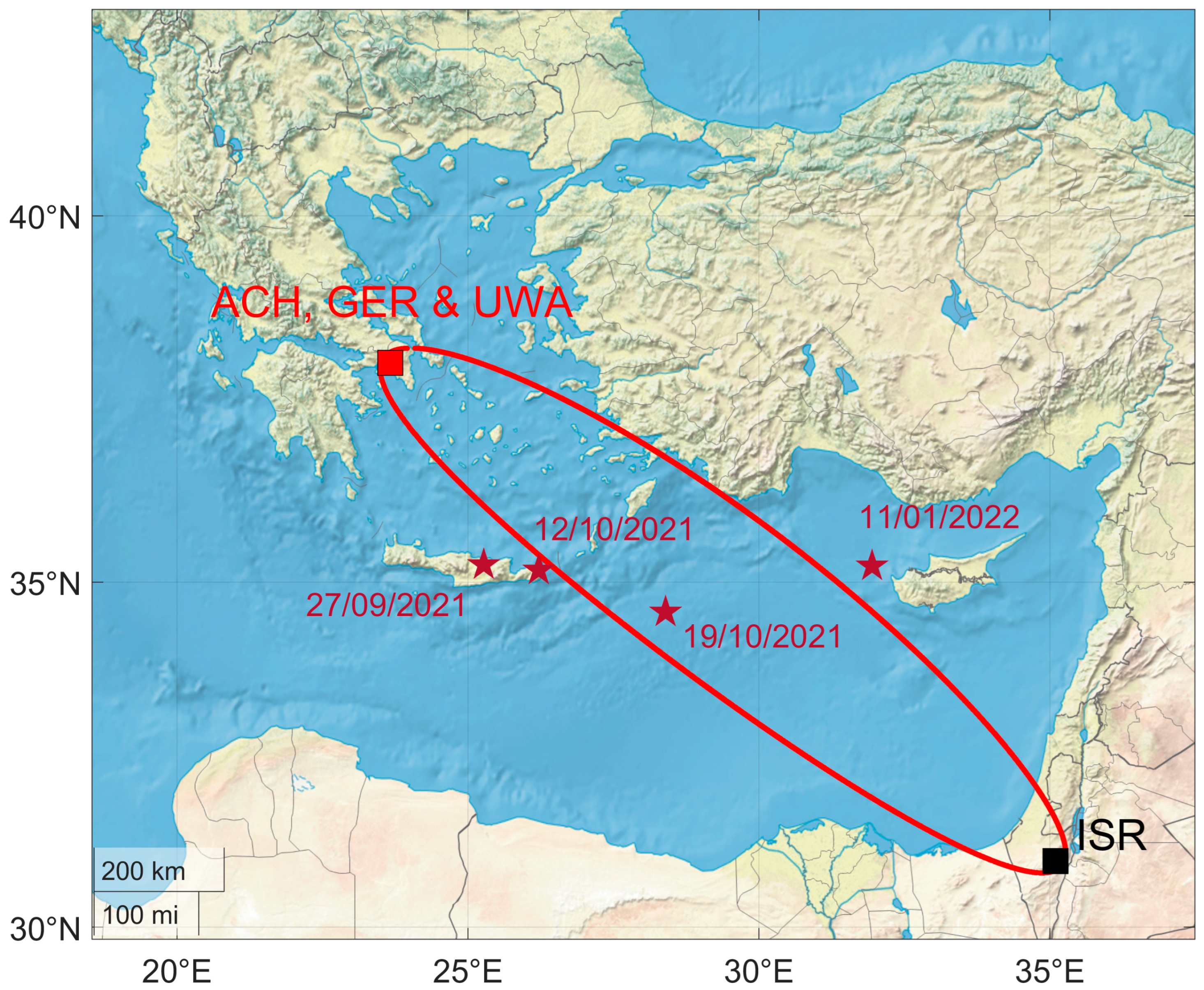
“EQ Group” Based on the Time Occurrence and the Location of the Epicenter of the Studied EQDate and Time
of Occurrence
(UT)
Magnitude   ( M L ) Depth (km)LatitudeLongitude
2021 Crete EQs27 September 2021 06:17:215.89.635.1521° N25.2736° E
2021 Crete EQs12 October 2021 09:24:026.310.434.8944° N26.4716° E
2021 Crete EQs19 October 2021 05:32:356.158.534.7131° N28.2532° E
2022 Cyprus EQ11 January 2022 01:07:496.434.735.1398° N31.9537° E
Table 2. Results of NFM for the 2022 Cyprus EQ. UWA, GER, and ACH denote the station where the corresponding anomaly in T R * , D P * ,   o r   N F * has been identified.
Date of Appearance of the Anomaly (UT)TR*DP*NF*Possibly Associated Extreme Event(s)
2 December 2021GERGERUWA, GER-
11 December 2021 GER b
21 December 2021 UWA b, c
4 January 2022ACHACH, GERACHa
5 January 2022UWA, ACH, GERACHUWA, ACH, GERa
27 January 2022 ACH -
The following letters appearing in the column “Possibly associated extreme event(s)” denote, respectively: a → 2022 Cyprus EQ (6.4 M L , 11 January 2022); b → a 5.6 M L EQ that occurred on 26 December 2021 18:59:02 (UT) at (35.2029° N, 26.8497° Ε); c → a 5.7 M L EQ that occurred on 29 December 2021 05:08:09 (UT) at (34.791° N, 25.139° Ε).
Table 3. Results of NFM for the 2021 Crete EQs. UWA and GER denote the station where the corresponding anomaly in T R * , D P * ,   o r   N F * has been identified.
Date of Appearance of the Anomaly (UT)TR*DP*NF*Possibly Associated Extreme Event(s)
5 September 2021UWAUWA, GERUWA, GER-
9 September 2021GERGERGERa
19 September 2021UWA, GER a
28 September 2021 GER b
4 October 2021 UWA b, c
7 October 2021UWA, GER UWA, GERb, c
9 October 2021 GER b, c
11 October 2021UWA UWA, GERc
12 October 2021 UWA c
27 October 2021UWA GER-
The following letters appearing in the column “Possibly associated extreme event(s)” denote, respectively: a → 1st 2021 Crete EQ (5.8 M L , 27 September 2021); b → 2nd 2021 Crete EQ (6.3 M L , 12 October 2021); c → 3rd 2021 Crete EQ (6.1 M L , 19 October 2021).
Table 4. Results from the diurnal sequential plots for the 2022 Cyprus EQ. UWA, GER, and ACH denote the station where the corresponding anomaly in t m 1 and/or t e has been identified.
Date of Appearance of the Anomaly (UT)Shift in
t m 1
Shift in
t e
Possibly Associated Extreme Event(s)
28 December 2021 UWA, GER, ACHa, b
1 January 2022UWA, GER, ACH b
2 January 2022GER, ACHGER, ACHb
3 January 2022 GER, ACHb
4 January 2022 GER, ACHb
5 January 2022 UWA,
GER, ACH
b
6 January 2022 UWA, GER, ACHb
7 January 2022 UWAb
8 January 2022UWA, GER, ACH b
9 January 2022UWA, GER, ACHUWA, GER, ACHb
The following letters appearing in the column “Possibly associated extreme event(s)” denote, respectively: a → a 5.7 M L EQ that occurred on 29 December 2021 05:08:09 (UT) at (34.791° N, 25.139° Ε); b → 2022 Cyprus EQ (6.4 M L , 11 January 2022).
Table 5. Results from diurnal sequential plots for 2021 Crete EQs. UWA and GER denote the station where the corresponding anomaly in TTs has been identified.
Date of Appearance of the Anomaly (UT)Shift in
t m 1
Shift in
t m 2
Shift in
t e 1
Shift in
t e 2
Possibly Associated Extreme Event(s)
13 September 2021 UWA, GERa
15 September 2021 UWAGERa
17 September 2021 GER a
18 September 2021 UWA, GER a
19 September 2021 UWA, GERUWA a
20 Septemebr 2021 UWA, GER a
21 September 2021UWA a
22 September 2021UWA a
24 September 2021UWA, GER UWA a
25 September 2021UWA UWA a
26 September 2021 UWA a
27 September 2021 UWA a, b
28 September 2021GER UWAUWAb
2 October 2021 GERGER b
3 October 2021 GER b
4 October 2021 GER b, c
6 October 2021 b, c
7 October 2021UWA, GER UWA b, c
8 October 2021 UWA b, c
9 October 2021 UWA b, c
10 October 2021UWA b, c
11 October 2021GER UWA, GER b, c
14 October 2021 GER c
15 October 2021 GER c
16 October 2021UWA c
17 October 2021UWA UWA c
The following letters appearing in the column “Possibly associated extreme event(s)” denote, respectively: a → 1st 2021 Crete EQ (5.8 M L , 27 September 2021); b → 2nd 2021 Crete EQ (6.3 M L , 12 October 2021); c → 3rd 2021 Crete EQ (6.1 M L , 19 October 2021).
Table 6. Results of TTM analysis for the 2022 Cyprus EQ. UWA, GER, and ACH denote the station where the corresponding anomaly has been identified.
Date of Appearance of the Anomaly (UT)Excess of
2 σ   for   d t m 1
Excess of
2 σ   for   d t m 2
Excess of
2 σ   for   d t e
Excess of
2 σ   for   d D V L F 1 1
Possibly Associated
Extreme Event(s)
7 December 2021 ACH (shifted −12.1 min) -
8 December 2021 UWA (shifted −19.6 min), GER (shifted −12.2 min) -
21 December 2021 UWA (shifted
−50.1 min)
b, c
28 December 2021 GER (shifted 26.9 min) a, c
1 January 2021UWA (shifted −34.7 min) a
6 January 2021 ACH (shifted 29.8 min) a
8 January 2021UWA (shifted −33.2 min), ACH (shifted −34.5 min), GER (shifted
−40.6 min)
a
9 January 2021 UWA (shifted
43.4 min), ACH (shifted
51.3 min), GER (shifted
53.9 min)
a
24 January 2021 UWA (shifted 34 min) -
The following letters appearing in the column “Possibly associated extreme event(s)” denote, respectively: a → 2022 Cyprus EQ (6.4 M L , 11 January 2022); b → a 5.5 M L EQ that occurred on 26 December 2021 18:59:02 (UTC) at (35.2029° N, 26.8497° Ε); c → a 5.7 M L EQ that occurred on 29 December 2021 05:08:09 (UTC) at (34.791° N, 25.139° Ε).
Table 7. Results of TTM analysis for the 2021 Crete EQs. UWA and GER denote the station where the corresponding anomaly has been identified.
Date of Appearance of the Anomaly (UT) Excess   of   2 σ for
d t m 1
Excess   of   2 σ for
d t m 2
Excess   of   2 σ for
d t e 1
Excess   of   2 σ for
d t e 2
Excess   of   2 σ for
d D V L F 1 1
Excess   of   2 σ for
d D V L F 1 2
Excess   of   2 σ for
d D V L F 2 1
Excess   of   2 σ for
d D V L F 2 2
Possibly Associated Extreme Event(s)
4 September 2021 UWA (shifted 34.5 min) UWA (shifted 35 min)UWA (shifted 35.83 min)-
6 September 2021 GER (shifted 52.5 min) GER (shifted 57 min)GER (shifted 47.75 min)a
19 September 2021 UWA (shifted 28.4 min) a
20 September 2021 UWA (shifted −13.7 min), GER (shifted −20.1 min) a
28 September 2021 UWA (shifted 26 min) UWA (shifted 26.3 min) b
1 October 2021 GER (shifted −18.75 min)UWA (shifted 36.9 min) UWA (shifted 32.5 min)UWA (shifted 39.1 min)b
2 October 2021 GER (shifted −35.66 min) GER (shifted 44.16 min) GER (shifted 38 min)b
7 October 2021UWA (shifted −45 min), GER (shifted −43.8 min) UWA (shifted 57.6 min) b, c
11 October 2021GER (shifted −32 min) UWA (shifted 26 min) GER (shifted 48.7 min) b, c
12 October 2021 UWA (shifted −10.87 min) b, c
The following letters appearing in the column “Possibly associated extreme event(s)” denote, respectively: a → 1st 2021 Crete EQ (5.8 M L , 27 September 2021); b → 2nd 2021 Crete EQ (6.3 M L , 12 October 2021); c → 3rd 2021 Crete EQ (6.1 M L , 19 October 2021).
Table 8. Results of the NT analysis for the 2022 Cyprus EQ. UWA, GER, and ACH denote the station where the corresponding criticality has been identified.
Date of Appearance of the Criticality Signature (UT)NT Analysis on TRNT Analysis on DPNT Analysis on NFPossibly Associated Extreme Event(s)
29 December 2021 UWA a
30 December 2021 GERACHa
4 January 2022 ACHa
7 January 2022UWA, GER a
8 January 2022ACH UWAa
10 January 2022 ACH a
15 January 2022UWA, GER b, c, d, e
20 January 2022GERGER f, g
22 January 2022ACHGER f, g
23 January 2022GER, ACHGER f, g
24 January 2022ACH f, g
25 January 2022GER, ACH UWAf, g
The following letters appearing in the column “Possibly associated extreme event(s)” denote, respectively: a → 2022 Cyprus EQ (6.4 M L , 11 January 2022); b → post-EQ power laws due to “locally surviving” critical dynamics, despite the unstable critical point no longer existing; c → a minor (Kp~5) geomagnetic storm that occurred on 15 January 2022 21:00:00 (UT); d → a minor (Kp = 5) geomagnetic storm that occurred on 18 January 2022 00:00:00 (UT); e → a minor (Kp = 5) geomagnetic storm that occurred on 19 January 2022 03:00:00 (UT); f → a minor (min Dst = −66 nT) geomagnetic storm that occurred on 3 February 2022 10:00:00 (UT); g → a minor (min Dst = −61 nT) geomagnetic storm that occurred on 4 February 2022 20:00:00 (UT).
Table 9. Results of the NT analysis for the 2021 Crete EQs. UWA and GER denote the station where the corresponding criticality has been identified.
Date of Appearance of the Criticality Signature (UT)NT Analysis on TRNT Analysis on DPNT Analysis on NFPossibly Associated Extreme Event(s)
9 September 2021GER a
10 September 2021 UWA, GER a
11 September 2021UWA a
12 September 2021UWA UWAa
19 September 2021 GERa
The following letter appearing in the column “Possibly associated extreme event(s)” denotes: a → 1st 2021 Crete EQ (5.8 M L , 27 September 2021).
Table 10. Results of wavelet analysis for the 2022 Cyprus EQ.
Receiver Call NameDate of Appearance of the Anomaly (UT)Time of Appearance of the Anomaly (UT)Range of Periodic Structures (min.)Intensity of the Wave-Like StructuresPossibly Associated Extreme Event(s)
UWA27 December 202121:45:57–22:24:0031–36moderatea, b
31 December 202122:10:48–23:21:0031–54higha
2 January 202100:07:48–00:54:0031–38moderatea
10 January 202121:43:48–23:07:4831–50moderatea
11 January 202121:45:36–22:27:0031–38moderatea
GER5 January 202221:37:48–22:12:3631–38higha
ACH9 January 202223:48:00–00:25:4831–36moderatea
10 January 202200:24:36–01:12:0031–41higha
The terms “high” and “moderate” in the column “Characterization of the intensity of power of the wave-like structures” verbally characterize the intensity of the wave-like structures with reference to the normalized linear scale of power (33–66% for “moderate” and 67–100% for “high”). The following letters appearing in the column “Possibly associated extreme event(s)” denote, respectively: a → 2022 Cyprus EQ; b → a 5.7 M L EQ that occurred on 29 December 2021 05:08:09 (UTC) at (34.791° N, 25.139° Ε).
Table 11. Results of wavelet analysis for the 2021 Crete EQs.
Receiver Call NameDate of Appearance of the AnomalyTime of Appearance of the Anomaly (UT)Range of Periodic Structures (min.)Intensity of the Wave-Like StructuresPossibly Associated Extreme Event(s)
UWA13 September 202122:48:36–00:22:4831–47moderatea
17 September 202122:52:48–00:43:4831–36higha
17 September 202123:21:00–00:36:0047–71moderatea
4 October 202122:07:48–00:31:4831–38highb, c
8 October 202123:21:36–00:27:0031–36highb, c
8 October 202122:54:36–00:01:4871–94highb, c
9 October 202123:45:36–00:57:0031–50moderateb, c
10 October 202121:58:48–00:55:4841–47moderateb, c
11 October 202123:46:48–01:09:0036–54highb, c
12 October 202123:04:48–00:21:0041–62moderateb, c
13 October 202123:46:48–01:49:4854–66moderatec
16 October 202122:09:36–23:18:3631–33moderatec
GER12 September 2021 00:00:00–00:45:3631–36higha
28 September 202122:43:48–00:09:3631–50highb
28 September 202122:58:48–00:22:4857–87moderateb
4 October 202123:03:36–00:24:3635–43highb, c
9 October 202123:36:36–01:00:0043–66highb, c
10 October 202100:03:00–01:09:3633–46moderateb, c
12 October 202123:33:36–00:18:0033–44moderateb, c
13 October 202122:36:00–23:54:3631–41moderatec
16 October 202121:42:36–00:09:0031–35highc
19 October 202121:43:48–00:33:3631–38highc
The terms “high” and “moderate” in the column “Characterization of the intensity of power of the wave-like structures” verbally characterize the intensity of the wave-like structures with reference to the normalized linear scale of power (33–66% for “moderate” and 67–100% for “high”). The following letters appearing in the column “Possibly associated extreme event(s)” denote, respectively: a → 1st 2021 Crete EQ (5.8 M L , 27 September 2021); b → 2nd 2021 Crete EQ (6.3 M L , 12 October 2021); c → 3rd 2021 Crete EQ (6.1 M L , 19 October 2021).
Disclaimer/Publisher’s Note: The statements, opinions and data contained in all publications are solely those of the individual author(s) and contributor(s) and not of MDPI and/or the editor(s). MDPI and/or the editor(s) disclaim responsibility for any injury to people or property resulting from any ideas, methods, instructions or products referred to in the content.

