Article

Short-Term Wind Speed Forecasting Based on the EEMD-GS-GRU Model

1
College of Resources and Environment, Yangtze University, Wuhan 430100, China
2
China Yangtze Power Co., Ltd., Yichang 443000, China
3
Hubei Key Laboratory of Intelligent Yangtze and Hydroelectric Science, Yichang 443000, China
4
State Grid Northwest Electric Power Dispatching Center, Xi’an 710048, China
*
Author to whom correspondence should be addressed.
Atmosphere 2023, 14(4), 697; https://doi.org/10.3390/atmos14040697
Submission received: 27 February 2023 / Revised: 1 April 2023 / Accepted: 6 April 2023 / Published: 7 April 2023
(This article belongs to the Special Issue Wind Forecasting over Complex Terrain)

Abstract

:
To improve the accuracy of short-term wind speed forecasting, we proposed a Gated Recurrent Unit network forecasting method, based on ensemble empirical mode decomposition and a Grid Search Cross Validation parameter optimization algorithm. In this study, first, in the process of decomposing, the set empirical mode of decomposition was introduced to divide the wind time series into high-frequency modal, low-frequency modal, and trend modal, using the Pearson correlation coefficient. Second, during parameter optimization, the grid parameter optimization algorithm was employed in the GRU model to search for the combination of optimal parameters. Third, the improved GRU model was driven with the decomposed components to predict the new components, which were used to obtain the predicted wind speed by modal reorganization. Compared with other models (i.e., the LSTM, GS-LSTM, EEMD-LSTM, and the EEMD-GS-LSTM), the proposed model was applied to the case study on wind speed of a wind farm, located in northwest China. The results showed that the presented forecasting model could reduce the forecasting error (RMSE) from 1.411 m/s to 0.685 m/s and can improve the accuracy of forecasts. This model provides a new approach for short-term wind speed forecasting.

1. Introduction

As China aims to reach its carbon peak in 2030 and to achieve its double carbon goal by 2060, it was estimated that the country’s electricity consumption will surpass 16 trillion kWh, with 80% of that energy being derived from carbon-free sources. The integration of wind power into the provision of energy will pose significant challenges to the capacity of the power grid [1], due to the intermittent and fluctuating nature of wind energy; therefore, the accurate forecasting of wind speed will play a crucial role in enabling the power system to effectively integrate and utilize wind power, to ensure the safe and stable operation of the grid.
In recent years, researchers have proposed a variety of wind speed forecasting and wind power forecasting methods. For instance, Ji L et al. [2] used the CNN-GRU model to predict the wind speed of canyons; experimental results showed that the proposed method improved MAE and RMSE by nearly 20%, which provided new ideas for the application of wind speed forecasting in canyons under complex terrain. Some studies have shown that signal analysis methods for the data preprocessing of wind speed time series can effectively reduce the impact of wind speed’s nonstationarity on forecasting results; therefore, the decomposition–reconstruction forecasting model, which has received an increasing amount of attention based on signal analysis methods [3]. In this model, the wind speed time series was decomposed into different modes using the mode decomposition algorithm to forecast. This could effectively reduce the complexity of the time series and eliminate the noise of the original data to enhance the forecast’s accuracy. For example, Ding et al. [4] used the ensemble empirical mode decomposition algorithm to decompose the wind power time series into several subsequences, and then predicted them separately, in combination with LSTM-SVR. This was seen to improve the system’s wind power absorption capacity and operating efficiency, while also achieving low-carbon emission goals. In addition, Gao et al. [5] used a Complementary Ensemble Empirical Mode Decomposition algorithm (CEEMD) to decompose the wind speed time series into different wind speed subsequences. After this, they established Extreme Learning Machine (ELM) models for the subsequences’ forecasting. The results showed that the accuracy of wind speed forecasting was improved. Furthermore, Chen et al. [6] used the K-means algorithm to cluster the wind speed time series on similar days, which they combined with the Variational Mode Decomposition algorithm (VMD) to decompose the wind speed series and then constructed a long short-term neural network. Long Short-Term Memory (LSTM) were the results of a combined forecasting model and they showed that combined models could effectively improve the accuracy of short-term wind speed forecasting. Jiang et al. [7] applied the Empirical Mode Decomposition (EMD) method to decompose the wind speed time series, and to obtain multiple intrinsic modal components. This enabled them to construct a Vector Autoregressive model (VAR) for each modal component of the forecasting. The experimental results showed that the accuracy of seasonal wind speed forecasts could be effectively improved. Nasiri et al. [8] decomposed the input signal to several IMFs by VMD, each of the IMFs was given to a separate MFRFNN for forecasting and predicted signals, which were summed to reconstruct the output; experimental results indicated that VMD-MFRFNN obtained better prediction results compared to the comparison model in the paper.
Although the above studies focused on the decomposition of the wind speed series, they neglected the hyperparameter selection of the neural network. Artificially selecting the hyperparameters of the network could not make a model’s forecasting optimal and consumed a lot of time. Therefore, other studies used smart algorithms to choose hyperparameters which improved forecasting accuracy. Some scholars have further proposed combined models forecasting, which included a parameter search algorithm. Wu et al. [9] combined the hybrid variational modal decomposition rain bat algorithm to optimize the Least Squares Support Vector Machine for the short-term forecasting of wind speed. This showed that VMD had a stronger decomposition ability than EEMD and that its forecasting accuracy was significantly better than the proposed comparison model. Li et al. [10] combined the EEMD method with the Backpropagation (BP) neural network, which was optimized by the flower pollination algorithm, to predict wind speed time series. This obtained a higher forecasting accuracy than that of the single model forecasting. Nasiri et al. [11] proposed a novel Multifunctional Recurrent Fuzzy Neural Network (MFRFNN) for chaotic time series forecasting and a new learning algorithm was developed which used the PSO algorithm for training the weights of MFRFNN. Overall, the experimental results showed that MFRFNN got a better accuracy rate on both chaotic benchmarks and real-world datasets. Li et al. [12] used the EEMD algorithm to decompose the wind power time series, and then the BI-LSTM after Bayesian optimization was established to predict the subsequences. This improved wind power forecasting accuracy. Nevertheless, few of the above studies decomposed the time series modalities and then divided the modalities into different types of modalities, which could improve the forecast accuracy when using neural networks to predict separately.
Based on the above literature review, the following gaps still exist in time series forecasting. Firstly, optimization algorithms were not commonly used in neural networks; some studies directly input wind speed time series into the neural network for forecasting. These methods could obtain great prediction results, but there is still scope to improve the prediction accuracy. Secondly, a part of studies used the same forecasting method for all subsequences after decomposition of wind speed time series, without considering the unique nature of each subsequence having different frequencies. Finally, existing artificial intelligence methods for wind speed forecasting always selected parameters through manual experience, which took a lot of time and not easy to match the optimal combination of parameters; it would affect the accuracy of wind speed forecasting. Therefore, the paper proposed a wind speed forecasting algorithm based on gated recurrent units and grid optimization search in an attempt to enhance existing forecasting models. Firstly, EEMD decomposed the original wind speed time series in the model preprocessing process, and several IMFs were obtained. Secondly, all components were separated into high-frequency, low-frequency, and trend modals based on the Pearson correlation coefficient method. Thirdly, the GRU model was established to predict the low, high, and trend subsequences, respectively. The Grid Search Cross Validation algorithm enhanced was used to optimize the GRU model. Finally, the forecasting for these components were summed to give the ultimate wind speed value. Experimental results have demonstrated that this model outperforms contrast models in this paper in terms of its forecasting accuracy.

2. Research Methods

2.1. Ensemble Empirical Mode Decomposition Method

In addressing nonstationary and nonlinear time series data, the empirical mode decomposition (EMD) method (first proposed in [13], in 1998) offered a means of processing signals by generating intrinsic mode functions. This approach eliminates the need for spurious harmonics in representing nonlinear and nonstationary signals and was effective in dealing with nonlinear time series data, such as wind speed and wind power, among others. The EMD technology was allowed for the extraction of different intrinsic mode functions (IMFs) and residuals, based on the local characteristics of the original data. The IMFs must satisfy two principles: (1) the number of local minimum extreme points and zero-crossing points must either be the same or differ by one, at the most; (2) the mean value of the upper and lower envelopes, whose local maximum and minimum must be equal zero.
While the EMD technology has demonstrated promising results, the IMFs generated from its decomposition may suffer from modal aliasing. To address this, the EEMD method—a noise-assisted data analysis approach—was proposed in [14]. This method has the advantage of adaptively extracting the signal components and changing trends, while also significantly reducing the modal aliasing phenomenon present in the EMD method [15]. The EEMD overcame the issue of false harmonics in the wavelet transforms by incorporating uniformly distributed white noise during the decomposition process, multiple times. This covered the noise in the signal with artificially added noise, resulting in more accurate envelopes. Additionally, averaging the decomposition results further reduced the impact of noise. The more the process was repeated, the lower the impact of noise on the decomposition [16].
The EEMD decomposition steps were as follows:
  • Set the overall average times, M.
  • Add white noise,  n i ( t ) , with a normal distribution to the original signal,  x ( t ) , to generate a new signal, as follows:
    x i t = x t + n i ( t )
    where  n i ( t )  represents the addition of a white noise sequence for the i-th time and  x i t  represents the additional noise signal of the i-th test,  i  = 1, 2, … M.
  • EMD decomposition was performed on the obtained noise-containing signal,  x i ( t ) , and the form of the respective IMF’s sum was obtained, as follows:
    x i t = j = 1 J c i , j t + r i , j ( t )
    where  c i , j t  was the  j -th IMF decomposed after adding white noise for the i-th time;  r i , j ( t )  was the residual function, which represents the average trend of the signal; and J was the IMF’s quantity.
  • Repeat steps 2 and 3 for M times, adding white noise signals with different amplitudes for each decomposition to obtain the set of the IMF, as follows:  c 1 , j t c 2 , j t  …  c M , j t  = 1, 2, …  J .
  • Using the principle that the statistical average value of uncorrelated sequences was zero, the above corresponding IMFs are subjected to collective averaging operations to obtain the final IMF after EEMD decomposition, as follows:
    c j t = 1 M i = 1 M c i , j t
    where  c j t  was the  j th IMF decomposed by EEMD,  i  = 1, 2, … M j  = 1, 2, … J.

2.2. Grid Search Cross Validation Parameter Optimization Method

In part of the time series forecasting projects, some authors wasted some time in choosing model hyperparameters by artificial experience. With the advancement of technology, there were many hyperparametric optimization algorithms used for neural networks, which could find the optimal combination of hyperparameters; Grid Search Cross Validation was one of these optimization algorithms. The performance of the model depended heavily on the values of the hyperparameters, but there was no way to know the optimal value of the hyperparameters in advance, and researchers would need to try all possible values to know the optimal value; performing this operation manually could be time and resource intensive. So, GridSearchCV was used to automatically adjust hyperparameters.
The Grid Search Cross Validation parameter optimization algorithm referred to gridding the variable area, evaluating it by traversing all of the given parameter combinations, and finally comparing and selecting the optimal parameter combination. The required parameters must be set to their optimization range, which could be combined with the size of the neural network loss function, and cross validation must be performed to find the best parameter combination for the neural network [17].
Cross validation (CV) was a statistical method that was used to verify the performance of classifiers. It divided the original data into training sets and test sets, first, by using the training set to train the network and, second, by using the verification set to test the training. The obtained model was used as the evaluation index of the model. Researchers often used K-fold CV to divide the original data into K groups (usually evenly divided) and to make each subset of data a verification set. The remaining K-1 subset of data was made into a training set so that the K models can be obtained. The average of the classification accuracy of the final verification set of these K models was used as the performance index of the classifier under this K-CV [18].
After setting the hyperparameter range of its neural network, it traversed various parameter combinations and conducted cross validation to determine the most effective parameters. In this study, five-fold cross validation was used to select the appropriate hyperparameters, as shown in the Figure 1.

2.3. Long Short-Term Memory Network

The Long Short-Term Memory (LSTM) [19] was a variation of the Recurrent Neural Network (RNN), which incorporated the concept of memory cells and gates to store and controlled the flow of information. This mechanism allowed for the long-term retention of information, avoiding the issue of information loss due to the lateral depth of the network. Furthermore, the gating mechanism in the memory unit addresses the gradient attenuation during the gradient descent, thus mitigating issues such as gradient disappearance and explosion during the model training.
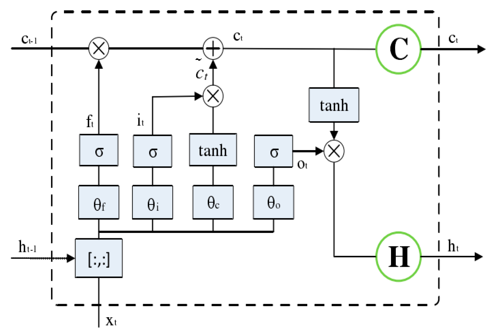
The internal specific structure of the LSTM neuron was shown in the figure below. In Figure 2, σ and tanh represent the sigmoid and tanh activation functions, respectively. The output range of the sigmoid between zero and one was used to simulate the opening of the gate. The output range of tanh between −1 and 1 was used for the normalization of the output. The input information flow enters between  h t 1  and  x t , and—through the control of the input, output, and forget gates—the memory unit,  c t 1 , was updated to  c t , and the neuron output,  h t , was also obtained.
Its calculation formula was as follows:
f t = s i g m o i d ( θ f · h t 1 , x t + b f )
i t = s i g m o i d ( · h t 1 , x t + b i )
o t = s i g m o i d ( θ o · h t 1 , x t + b o )
c t ~ = t a n h ( θ c · h t 1 , x t + b c )
c t = f t c t 1 + i t c t
h t = o t t a n h ( c t )
where  x t R d  is the input vector of the LSTM unit;  f t ( 0,1 ) h  is the activation vector of the forget gate;  i t ( 0,1 ) h  is the input/update gate activation vector;  o t ( 0,1 ) h  is the activation vector of the output gate;  h t ( 1,1 ) h  is the hidden state vector—also known as the output vector of the LSTM unit;  c t ~ ( 1,1 ) h  is the input activation vector of the cell; and  c t R h  is the cell state vector.

2.4. Gated Recurrent Unit

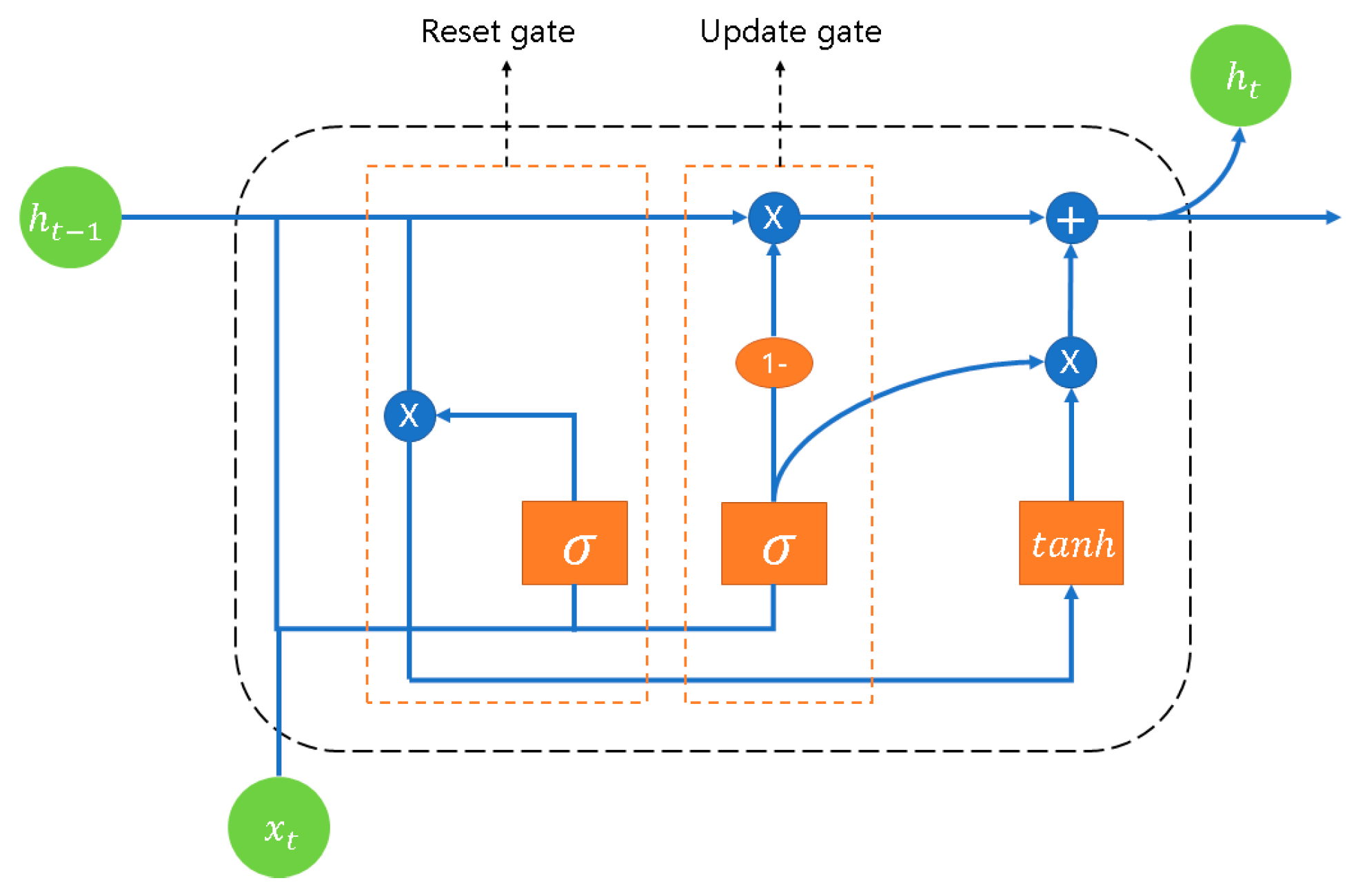
The Gated Recurrent Unit (GRU) network [20] was an optimized and simplified version of the long short-term memory (LSTM) network. The GRU network incorporated improvements to the forget and input gates, which were present in the LSTM network, by combining them into a single update gate. In this study, this update gate was used to determine the retention degree of the previous state information. The larger the update gate value, the higher the retention degree. The GRU network has several advantages over the LSTM network, including reduced training parameters, faster learning times, and, in many cases, improved forecasting performance. The structural unit of the GRU network was depicted in Figure 3, and its calculation formula could be represented as follows:
r t = σ x t W x r + H t 1 W h r + b r
z t = σ ( x t W x z + H t 1 W h z + b z )
H t ~ = tan h x t W h x + R t H t 1 W h h + b h
H t = ( 1 Z t ) H t 1 + Z t H t ~
where σ is a sigmoid function, and its output range is between zero and one;  H t 1  contains past information;  R t  is a reset gate; ⊙ is the element-wise multiplication;  H t ~  is a candidate hidden state; and  Z t  is the update gate.

3. Wind Speed Forecasting Model

3.1. EEMD-GS-GRU Modeling Process

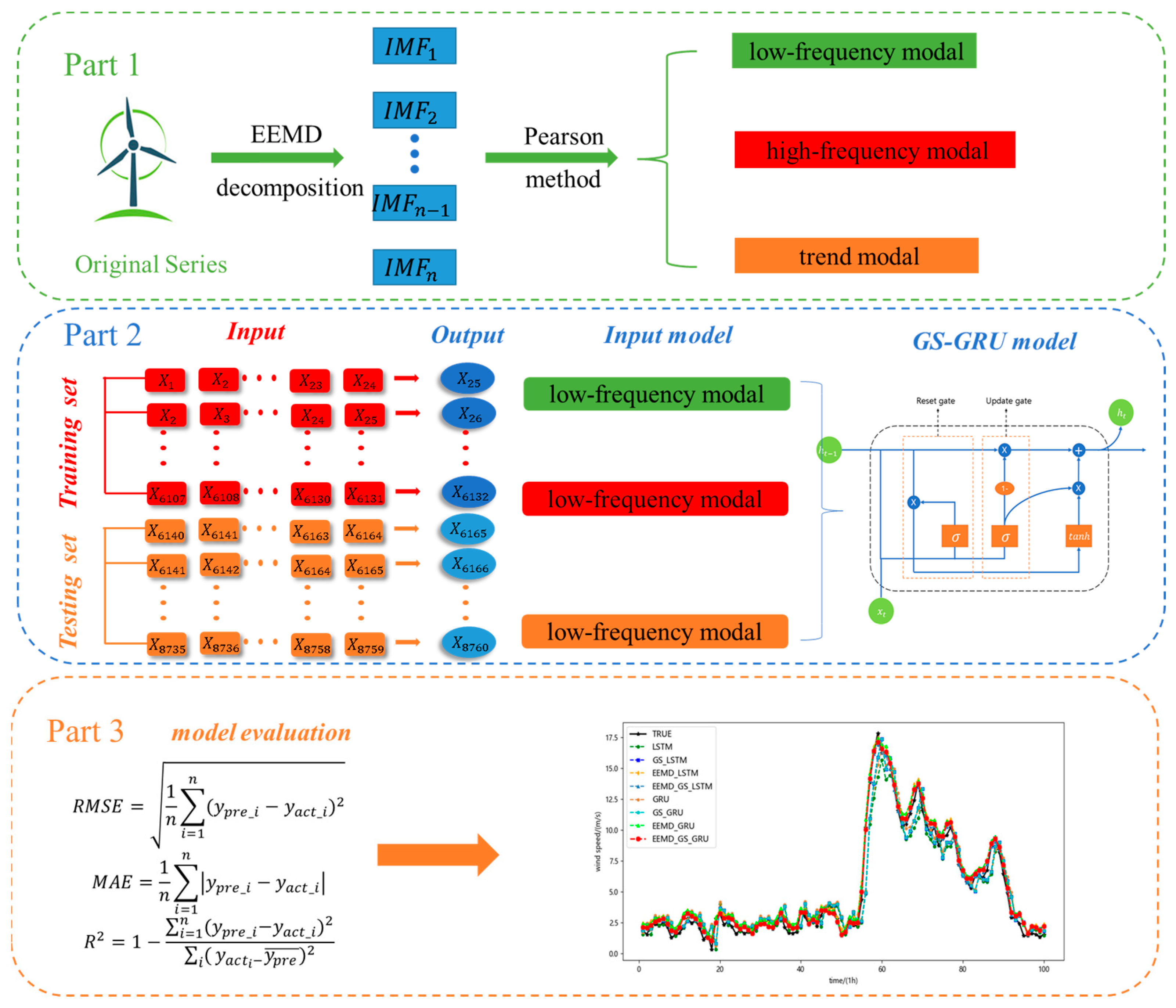
Considering the uncertainty and seasonality of wind speed, it was difficult to make accurate forecasts; therefore, in this paper, the time series was decomposed by EEMD, and the GS-GRU model was constructed for forecasting. The specific steps in this process were as follows:
  • EEMD was decomposed the original wind speed time series into subsequences.
  • According to the modes decomposed in (1), the low-frequency, high-frequency, and trend components were judged, and the models were established for forecasting.
  • The results of each subsequence predicted in (2) were superimposed to obtain the final result of the wind speed forecasting.
The model forecasting process was shown in Figure 4.

3.2. Predictive Evaluation Index

Mean absolute error “MAE”, coefficient of determination “ R 2 ”, and root mean square error “RMSE” were used to assess the stability of the model outcomes. “MAE” was a measure of errors between paired observations expressing the same phenomenon. “MAE” was calculated as the sum of absolute errors divided by the sample size. “ R 2 ”, known as the “goodness of fit”, was used to evaluate models’ accuracy.  R 2  ranges from 0 to 1 ( R 2  closer to 1 represents high model reliability). In general,  R 2  is the proportion of the variance in the output that was predictable from the input variables [21].
In this study, to quantitatively compare the forecasting results, we used the root mean square error (RMSE), the mean absolute error (MAE), and then  R 2  to evaluate the formula, as follows:
R M S E = 1 n i = 1 n ( y p r e _ i y a c t _ i ) 2
M A E = 1 n i = 1 n y p r e _ i y a c t _ i
R 2 = 1 i = 1 n ( y p r e _ i y a c t _ i ) 2 i ( y a c t i y p r e ¯ ) 2
where  n  was the number of sample points;  y a c t _ i  was the actual value at the time step, i y p r e _ i  was the predicted value at time step, i; and  y p r e ¯  was the mean of the sample forecasting.

3.3. Case Analysis

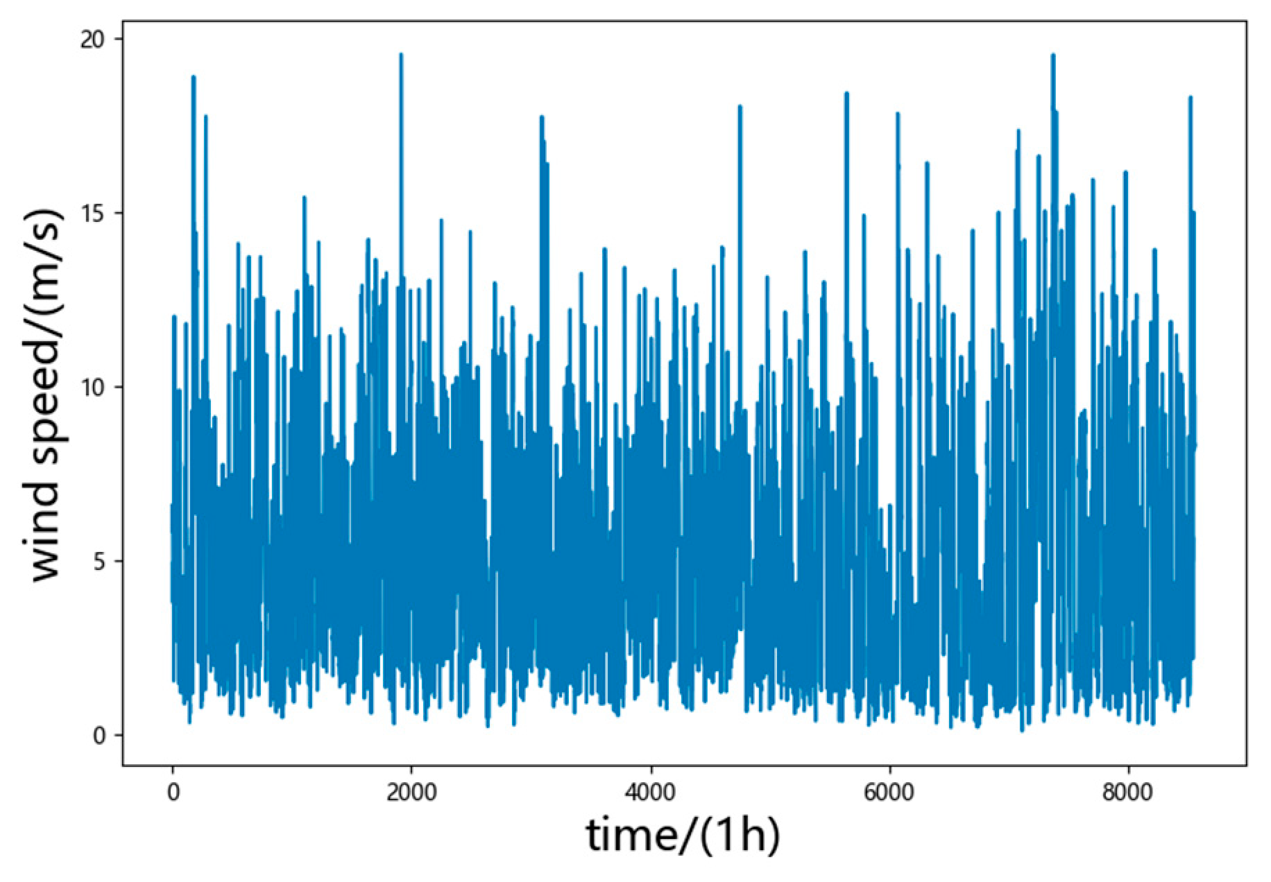
In this calculation example, we used the measured wind speed data from a wind farm in northwest China, from 1 March 2020 to 28 February 2021, as the example analysis. The data interval was 1 h, with a total of 8760 pieces of data. In total, 0.2% of the data were missing, so the data were completed using the linear interpolation method. The wind speed time series was shown in the Figure 5.
In statistics, the Pearson correlation coefficient was also known as Pearson’s r, which was a measure of linear correlation between two sets of data. It was the ratio between the covariance of two variables and the product of their standard deviations; thus, it was essentially a normalized measurement of the covariance, such that the result always has a value between −1 and 1. After decomposing the original wind speed time series by EEMD, the Pearson correlation coefficient method would be used for the decomposed time series. The correlation coefficients of each subsequence with the original wind speed were shown in Table 1 below. The EEMD decomposition of the above time series and the introduction of Gaussian noise were decomposed into 12 IMFs, of which IMF1-IMF6 were high-frequency components, IMF7-IMF10 were low-frequency components, and IMF11-IMF12 were trend components. These models were shown in Figure 6.
The EEMD algorithm was used to decompose the mode of the original wind speed time series, and the Pearson correlation coefficient was used to calculate the correlation with the original data and to classify it into low-frequency modal, high-frequency modal. Finally, each mode was predicted separately, and the superposition was performed after the forecasting was completed.
The wind speed time series contained a total of 8760 sample points. In this study, the first 70% of the data—namely, 6132 pieces of data—were used as the training set, and the last 30% of the data—namely, 2628 pieces of data—were used as the test set. According to the parameter tuning experiment and the grid parameter optimization algorithm, the hyperparameters of the network model were set, as shown in Table 2—where the time step unit was 1 h and 24 historical wind speed samples were used to predict the wind speed in the next 1 h. The LSTM network consisted of two LSTM layers; Dense fully connected the layers, and Composition set the dropout layer after the LSTM layer to prevent overfitting. Meanwhile, the GRU network consisted of two GRU layers; Dense fully connected the layers, and Composition set the dropout layer after the GRU layer to prevent overfitting. The experiments were run on an Intel Core i7-12700H, 2.30 GHz CPU with 16 GB RAM, and an Nvidia RTX 3060Ti GPU. The run times for all models are shown in Table 3 below. The parameters of models were as shown in Table 4.
To verify the feasibility of the model proposed in this study, the following models were constructed to compare their forecasting accuracy:
Model I (LSTM): we input the wind speed time series directly into the LSTM model for forecasting.
Model II (GS-LSTM): we input the wind speed time series into the LSTM model and combine the GS parameters to adjust the parameters for forecasting.
Model III (EEMD-LSTM): first, we decomposed the original wind speed time series into EEMD, and then we established LSTM models for forecasting.
Model IV (EEMD-GS-LSTM): first, we decomposed the original wind speed series into EEMD, and then we established the GS-LSTM model for forecasting.
Model V (GRU): we input the wind speed time series directly into the GRU model for forecasting.
Model VI (GS-GRU): we input the wind speed time series into the GRU model and combined it with GS parameter adjustment for forecasting.
Model VII (EEMD-GRU): first, we decomposed the original wind speed time series into EEMD and then we established a GRU model for forecasting.
Model VIII (EEMD-GS-GRU): first, we decomposed the original wind speed time series into EEMD and then we established the GS-GRU model for forecasting.
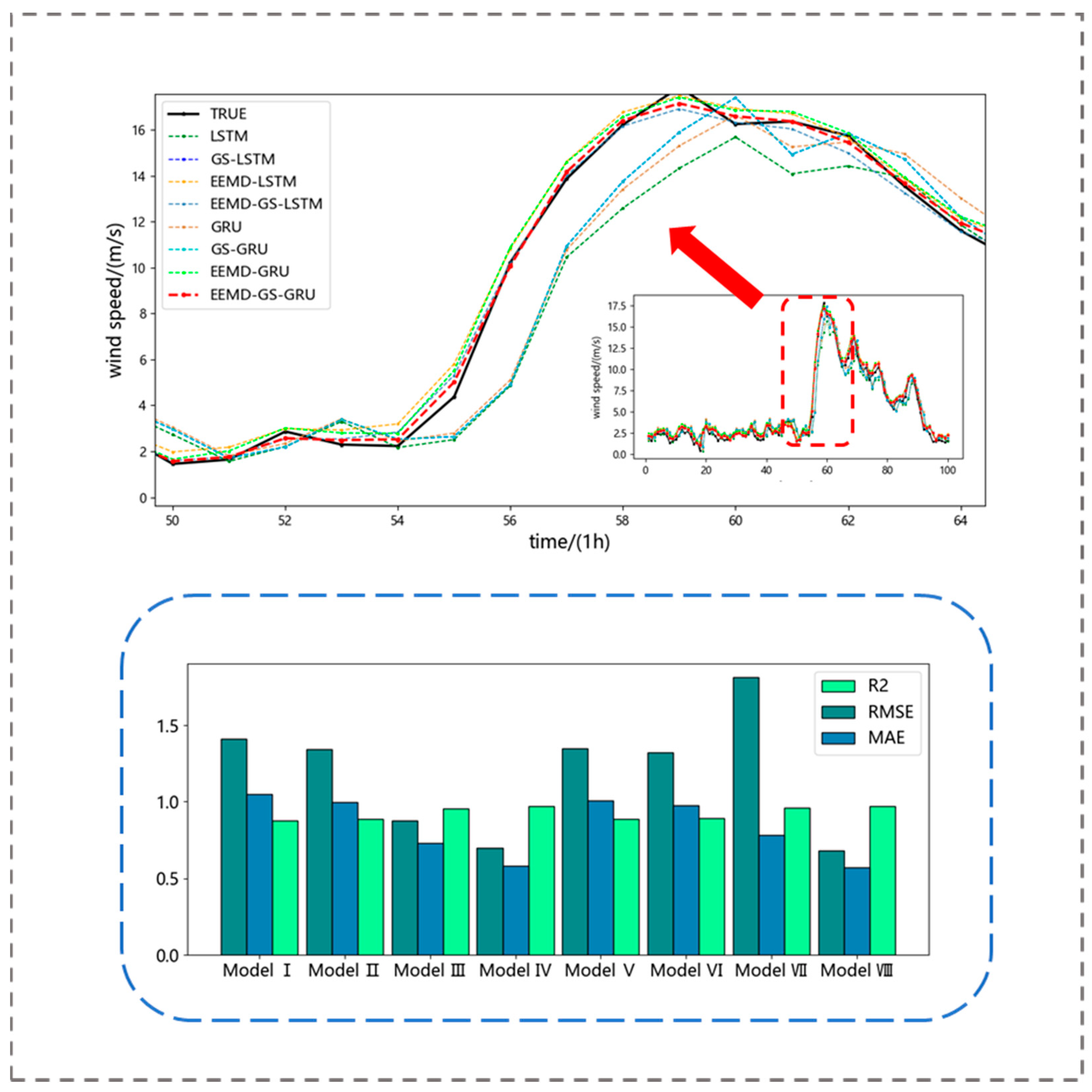
Due to the uncertainty of the deep learning algorithm, there may be some bias in its prediction results each time, so this would lead to some defects in the testing process of the proposed model. To increase the feasibility of the model proposed in this paper, five pre-experiments were conducted on the above eight models. The average value of the five pre-experiments was taken as the forecasting result. The forecasting results were shown in Table 5, below, and the forecasting comparison chart was shown in Figure 7, below.
Experimental results could be concluded from the eight models constructed in this paper, which could predict the overall trend of wind speed. Moreover, it could be seen that the forecasting accuracy of Model VIII (EEMD-GS-GRU) was better than the accuracy of the other seven models. Through the careful analysis of Table 3 and Figure 7, the following conclusions can be drawn:
(a)
By comparing the basic Model I (LSTM) and Model V (GRU) models, it could be found that the forecasting effect of the GRU model used in this paper was slightly better than the LSTM model.
(b)
Comparing the error metrics of Model V (GRU) and Model VII (EEMD-GRU), in the forecast result for test set, it could be found that the RMSE, MAE, and  R 2  of EEMD-GRU were reduced by 39.51%, 22.54% respectively, and  R 2  was improved by 7.99%. This indicated that the introduction of the ensemble empirical mode decomposition method (EEMD) into the forecasting of wind speed time series could significantly improve the forecasting accuracy of the model.
(c)
In wind speed forecasting, the algorithm-optimized Model II (GS-LSTM) and Model VI (GS-GRU) performed better than a single model. Taking the forecasting statistical measures of wind farm which used LSTM and GRU models, respectively, as an example, the RMSE of GS-LSTM was reduced by 4.96%, MAE was reduced by 5.04%, and  R 2  was increased 1.37%. The RMSE of GS-GRU is reduced 1.85%, MAE was reduced by 2.15%, and  R 2  was increased 0.5%. This showed that adding algorithm optimization could improve the forecast performance of the model; it meant the algorithm was better able to find neural network parameters to achieve better forecasting results.
(d)
From the forecast statistical error, compared with the Model V (GRU) and Model VIII (EEMD-GS-GRU), the RMSE and MAE of EEMD-GS-GRU were reduced by 48.26% and 43.29%, respectively, and  R 2  was increased by 9.34%. It shows that the composite model combining the modal decomposition and the optimization search algorithm was more suitable for wind speed forecasting.
(e)
Comparing the indicators of the Model IV (EEMD-GS-LSTM) and Model VIII (EEMD-GS-GRU), it could be seen that three error indicator values of the hybrid models using GRU model were slightly better than using the LSTM hybrid model. This suggested that the GRU method was more suitable for the forecasting of wind speed, which could track the wind speed time series more effectively. As a result, the hybrid model proposed in this study was suitable for the forecasting of wind speed.
To sum up, the forecasting performance of the model suggested in this research was superior to common benchmark models. However, the GS method proposed in this paper has some disadvantages. When the data set was large, training the model would consume a lot of time; this would be a waste of computing power. When the data set was small, the GS method could improve the wind speed forecasting. Overall, the method proposed could improve the accuracy of wind speed forecasting.

4. Conclusions

In this study, a wind speed forecasting model based on EEMD-GS-GRU has been proposed, and the following conclusions were obtained through an example analysis and through model comparison, as follows:
(1)
The grid parameter optimization algorithm was combined with the GRU model to predict the wind speed, and the forecasting accuracy was slightly improved.
(2)
The original wind speed time series was decomposed by EEMD, which could effectively reduce the influence of wind speed nonlinearity, intermittency, and instability on wind speed forecasting; therefore, the accuracy of the wind speed forecasting was improved.
(3)
We decomposed the original wind speed time series into high-frequency components, low-frequency components, and trend quantities through EEMD, and we performed GS-LSTM and GS-GRU modeling and forecasting on them, respectively. After this, the forecasting accuracy was improved, to some extent. Therefore, the model presented in this study can more clearly reflect the characteristics of the wind speed time series.
This study used nearly one year’s worth of historical wind speed data to build the model and verify it. Wind speed was affected by many meteorological factors. Therefore, in future studies, we will include more meteorological information as input data and use more advanced time series decomposition algorithms to further enhance the accuracy of the model’s wind speed forecasting.

Author Contributions

Conceptualization, H.Y., X.Z. and X.W.; methodology, H.Y. and X.W.; formal analysis, H.Y., Y.T. and X.W.; investigation, Y.T. and X.W.; resources, X.W.; data curation, Y.T., J.H. and Y.L.; writing—original draft preparation, Y.T., J.H. and Y.L. and X.W.; writing—review and editing, H.Y., Y.T., X.Z. and X.W.; visualization, Y.T., J.H. and Y.L.; supervision, H.Y.; funding acquisition, H.Y. and X.W. All authors have read and agreed to the published version of the manuscript.

Funding

This research was funded by the Program of the National Natural Science Foundation of China, grant number 51979198 and 91647204.

Institutional Review Board Statement

Not applicable.

Informed Consent Statement

Not applicable.

Data Availability Statement

Data is unavailable due to privacy restriction.

Conflicts of Interest

The authors declare no conflict of interest.

References

  1. Shu, Y. Developing new power systems to help achieve the goal of “double carbon”. China Power Enterp. Manag. 2021, 7, 8–9. [Google Scholar]
  2. Ji, L.; Fu, C.; Ju, Z.; Shi, Y.; Wu, S.; Tao, L. Short-Term canyon wind speed prediction based on CNN—GRU transfer learning. Atmosphere 2022, 13, 813. [Google Scholar] [CrossRef]
  3. Zhang, Y.; Han, P.; Wang, D. Short-term Wind Speed Prediction of Wind Farm Based on Variational Mode Decomposition and LSSVM. Sol. Energy J. 2018, 39, 194–202. [Google Scholar]
  4. Ding, C.; Zhou, Y.; Ding, Q. Integrated carbon-capture-based low-carbon economic dispatch of power systems based on EEMD-LSTM-SVR wind power forecasting. Energies 2022, 15, 1613. [Google Scholar] [CrossRef]
  5. Gao, G.; Yuan, K.; Zeng, X. Short-Term wind speed prediction based on improved CEEMD-CS-ELM. Sol. Energy J. 2021, 42, 284–289. [Google Scholar]
  6. Chen, C.; Zhao, X.; Bi, G. Short-Term Wind Speed Prediction Based on Kmeans-VMD-LSTM. Mot. Control. Appl. 2021, 48, 85–93. [Google Scholar]
  7. Nasiri, H.; Ebadzadeh, M.M. Multi-step-ahead Stock Price Prediction Using Recurrent Fuzzy Neural Network and Variational Mode Decomposition. arXiv 2022, arXiv:2212.14687. [Google Scholar]
  8. Jiang, Z.; Che, J.; Wang, L. Ultra-short-term wind speed forecasting based on EMD-VAR model and spatial correlation. Energy Convers. Manag. 2021, 250, 114919. [Google Scholar] [CrossRef]
  9. Wu, Q.; Lin, H. Short-term wind speed forecasting based on hybrid variational mode decomposition and least squares support vector machine optimized by bat algorithm model. Sustainability 2019, 11, 652. [Google Scholar] [CrossRef] [Green Version]
  10. Li, H.; Ren, Y.; Gu, R. Combined Wind Speed Prediction Based on Flower Pollination Algorithm. Sci. Technol. Eng. 2020, 20, 1436–1441. [Google Scholar]
  11. Nasiri, H.; Ebadzadeh, M.M. MFRFNN: Multi-Functional Recurrent Fuzzy Neural Network for Chaotic Time Series Prediction. Neurocomputing 2022, 507, 292–310. [Google Scholar] [CrossRef]
  12. Li, J.; Wang, Y.; Chang, J. Ultra-short-term prediction of wind power based on parallel machine learning. J. Hydroelectr. Power Gener. 2023, 42, 40–51. [Google Scholar]
  13. Huang, N.E.; Shen, Z.; Long, S.R.; Wu, M.C.; Shih, H.H.; Zheng, Q.; Liu, H.H. The empirical mode decomposition and the Hilbert spectrum for nonlinear and non-stationary time series analysis. Proceedings of the Royal Society of London. Ser. A Math. Phys. Eng. Sci. 1998, 454, 903–995. [Google Scholar] [CrossRef]
  14. Wu, Z.; Norden, E.H. Ensemble empirical mode decomposition: A noise-assisted data analysis method. Adv. Adapt. Data Anal. 2009, 1, 1–41. [Google Scholar] [CrossRef]
  15. Wu, Z.; Wu, N.; Huang, S.E.; Long, R. On the trend, detrending, and variability of nonlinear and nonstationary time series. Proc. Natl. Acad. Sci. USA 2007, 104, 14889–14894. [Google Scholar] [CrossRef] [Green Version]
  16. Sun, S.; Fu, J.; Li, A. A compound wind power forecasting strategy based on clustering, two-stage decomposition, parameter optimization, and optimal combination of multiple machine learning approaches. Energies 2019, 12, 3586. [Google Scholar] [CrossRef] [Green Version]
  17. Wen, B.; Dong, W.; Xie, W. Random Forest Parameter Optimization Based on Improved Grid Search Algorithm. Comput. Eng. Appl. 2018, 54, 154–157. [Google Scholar]
  18. Wang, J.; Zhang, L.; Chen, G. SVM parameter optimization based on improved grid search method. Appl. Sci. Technol. 2012, 39, 28–31. [Google Scholar]
  19. Hochreiter, S.; Schmidhuber, J. Long short-term memory. Neural Comput. 1997, 9, 1735–1780. [Google Scholar] [CrossRef] [PubMed]
  20. Dey, R.; Salem, F.M. Gate-variants of gated recurrent unit (GRU) neural networks. In Proceedings of the 2017 IEEE 60th International Mid-West Symposium on Circuits and Systems (MWSCAS), Boston, MA, USA, 6–9 August 2017; IEEE: Piscatway, NJ, USA, 2017; pp. 1597–1600. [Google Scholar]
  21. Chelgani, S.C.; Nasiri, H.; Alidokht, M. Interpretable modeling of metallurgical responses for an industrial coal column flotation circuit by XGBoost and SHAP-A “conscious-lab” development. Int. J. Min. Sci. Technol. 2021, 31, 1135–1144. [Google Scholar] [CrossRef]
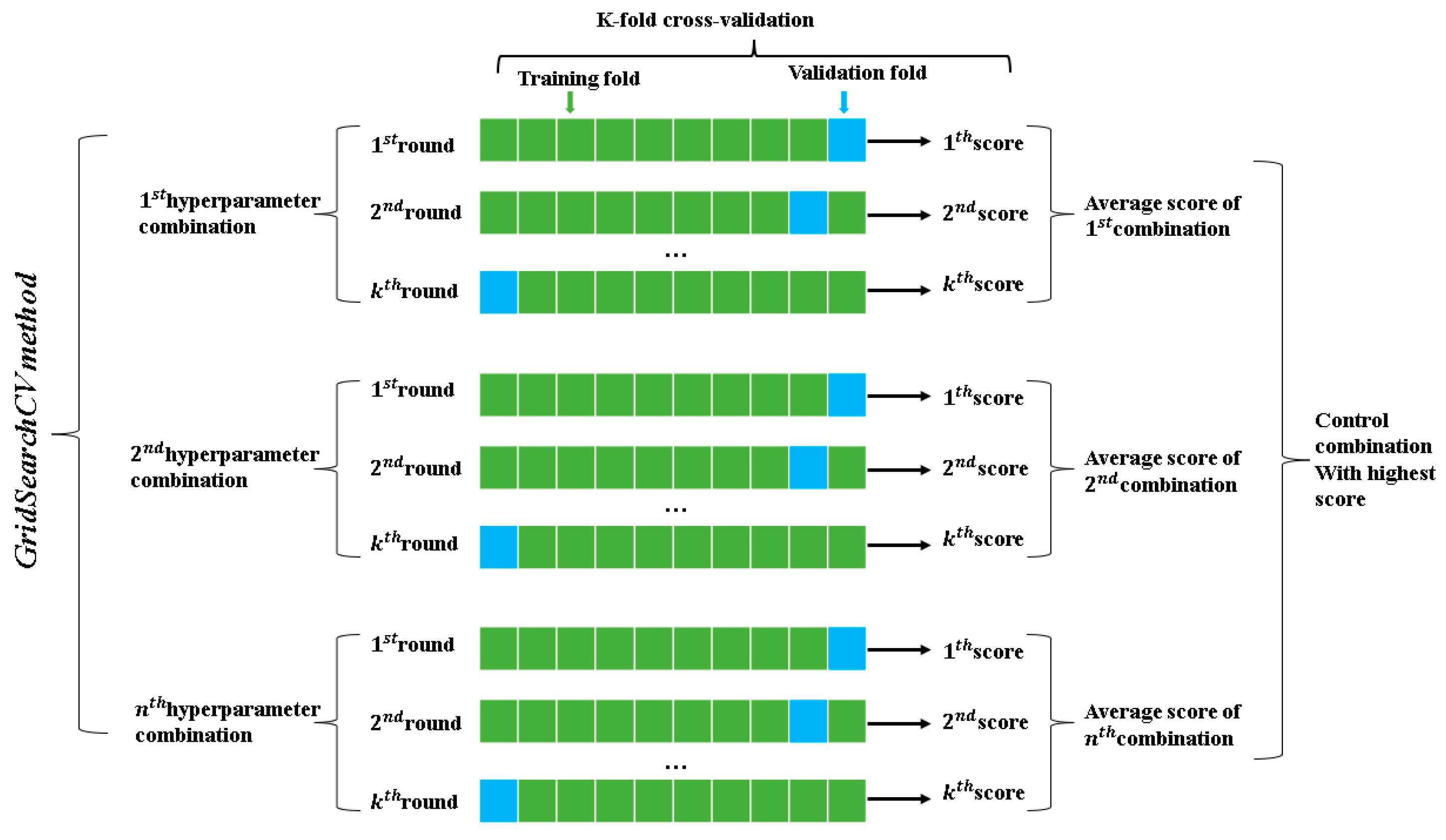
Figure 1. Schematic diagram of grid parameter optimization algorithm.
Atmosphere 14 00697 g001
Figure 2. Long short-term neural network diagram.
Atmosphere 14 00697 g002
Figure 3. Gated recurrent unit network diagram.
Atmosphere 14 00697 g003
Figure 4. EMMD-GS-GRU forecasting process.
Atmosphere 14 00697 g004
Figure 5. Original wind speed time series and rose chart.
Atmosphere 14 00697 g005
Figure 6. High−frequency modal, low−frequency modal, and trend components.
Atmosphere 14 00697 g006
Figure 7. Comparison of evaluation indicators.
Atmosphere 14 00697 g007
Table 1. Table of correlation coefficients.
IMF NameCorrelation Coefficients
IMF10.223 ***
IMF20.364 ***
IMF30.579 ***
IMF40.630 ***
IMF50.531 ***
IMF60.418 ***
IMF70.290 ***
IMF80.234 ***
IMF90.136 ***
IMF100.123 ***
IMF110.090 ***
IMF120.064 ***
Note: *** represents a significance level of 1%.
Table 2. Grid search algorithm parameter setting.
Hyperparameter Grid Search Range
Batch size[8, 16, 24, 32, 64]
Epoch[10, 15, 20, 25, 30]
Optimization[adam, Adadelta, SGD]
Table 3. The running time of model.
Model Name Running Time
LSTM3′16″
GS-LSTM8′20″
EEMD-LSTM25′46″
EEMD-GS-LSTM115′25″
GRU3′28″
GS-GRU8′36″
EEMD-GRU26′34″
EEMD-GS-GRU117′23″
Table 4. Parameters and values of Models.
Hyperparameter NameBatch SizeDropoutEpochOptimization
Model I240.225Adam
Model I160.230Adam
Model III240.225Adam
Model IV160.230Adam
Model V240.220Adam
Model VI160.230Adam
Model VII240.225Adam
Model VIII160.230Adam
Table 5. Comparison of four model evaluation indicators.
Evaluation IndexR2RMSE (m/s)MAE (m/s)
Model I0.8771.4111.051
Model II0.8891.3410.998
Model III0.9530.8760.729
Model IV0.9700.6960.581
Model V0.8881.3491.007
Model VI0.8921.3240.978
Model VII0.9590.8160.78
Model VIII0.9710.6850.571
Disclaimer/Publisher’s Note: The statements, opinions and data contained in all publications are solely those of the individual author(s) and contributor(s) and not of MDPI and/or the editor(s). MDPI and/or the editor(s) disclaim responsibility for any injury to people or property resulting from any ideas, methods, instructions or products referred to in the content.