
Data-Driven Air Quality and Environmental Evaluation for Cattle Farms


Abstract
:1. Introduction
2. Related Work
2.1. Technology and Solution Survey
2.2. Literature Survey
- Remote sensing data;
- Satellite dataset;
- Air pollution data;
- Cattle farm data.
3. Data Engineering
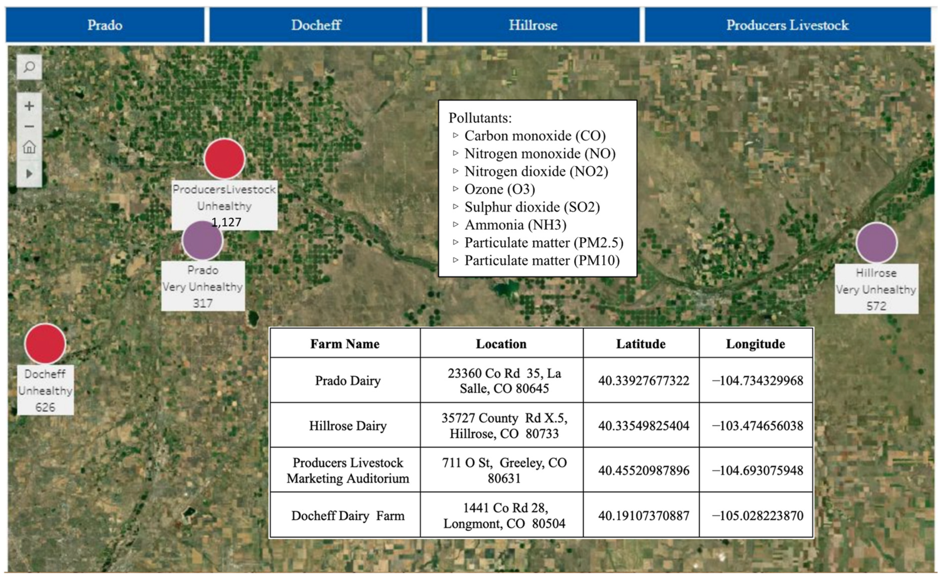
3.1. Study Area
3.2. Data Process
- Cattle detection and counting, which requires satellite data;
- Air pollutants based on coordinates, which requires remote sensing API.
3.2.1. Satellite Data
3.2.2. Remote Sensing Data
3.3. Data Collection
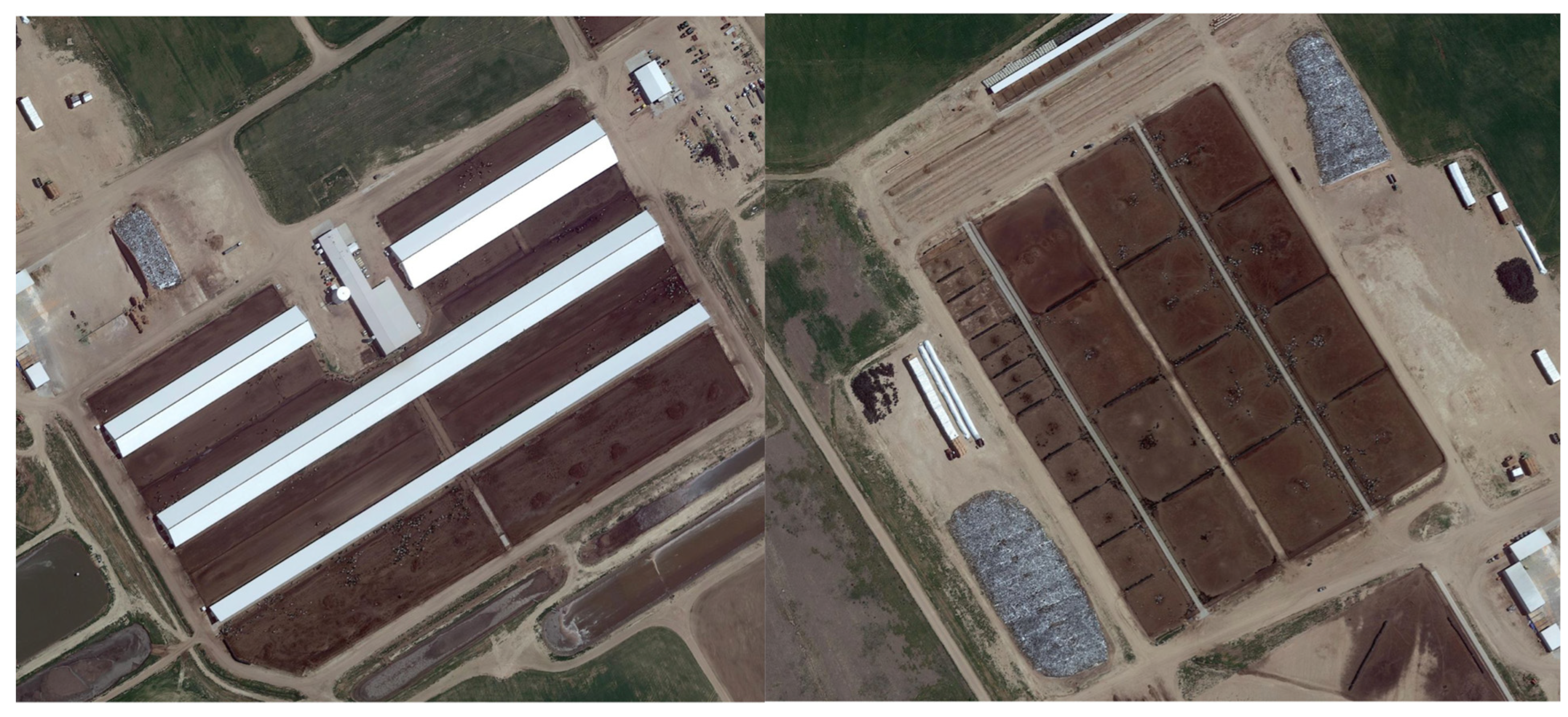
3.3.1. Cattle Count
3.3.2. Air Pollutants
- Carbon monoxide (CO);
- Nitrogen dioxide (NO2);
- Ozone (O3);
- Sulfur dioxide (SO2);
- Ammonia (NH3);
- Particulate matter (PM2.5);
- Particulate matter (PM10).
3.4. Data Pre-Processing
3.5. Data Transformation
3.5.1. Stage 1—Satellite Imagery Dataset
3.5.2. Stage 2—Remote Sensing Data
3.6. Data Preparation
3.7. Data Statistics
4. Model Development
4.1. Model Proposal
4.2. Model Supports
4.3. Model Comparison
4.4. Model Evaluation
4.5. Two-Stage Model Experimental Results
4.5.1. Stage One Modeling Results
Detectron2
YOLOv4
YOLOv5
RetinaNet
4.5.2. Stage Two Modeling
5. System Development
5.1. System Requirements Analysis
5.2. System Design
6. Conclusions
6.1. Summary
6.2. Recommendations for Future Work
Author Contributions
Funding
Institutional Review Board Statement
Informed Consent Statement
Data Availability Statement
Conflicts of Interest
References
- Lutz, W.; KC, S. Dimensions of global population projections: What do we know about future population trends and structures? Philos. Trans. R. Soc. B Biol. Sci. 2010, 365, 2779–2791. [Google Scholar] [CrossRef] [PubMed]
- Greenwood, P.L. An overview of beef production from pasture and feedlot globally, as demand for beef and the need for sustainable practices increase. Animal 2021, 15, 100295. [Google Scholar] [CrossRef]
- Bogaerts, M.; Cirhigiri, L.; Robinson, I.; Rodkin, M.; Hajjar, R.; Junior, C.C.; Newton, P. Climate change mitigation through intensified pasture management: Estimating greenhouse gas emissions on cattle farms in the Brazilian Amazon. J. Clean. Prod. 2017, 162, 1539–1550. [Google Scholar] [CrossRef]
- Thumba, D.; Lazarova-Molnar, S.; Niloofar, P. Estimating Livestock Greenhouse Gas Emissions: Existing Models, Emerging Technologies and Associated Challenges. In Proceedings of the 2021 6th International Conference on Smart and Sustainable Technologies (SpliTech), Bol and Split, Croatia, 8–11 September 2021. [Google Scholar] [CrossRef]
- Castelli, M.; Clemente, F.; Popovič, A.; Silva, S.; Vanneschi, L. A Machine Learning Approach to Predict Air Quality in California. Complexity 2020, 2020, 8049504. [Google Scholar] [CrossRef]
- Borlée, F.; Yzermans, C.J.; Aalders, B.; Rooijackers, J.; Krop, E.; Maassen, C.B.M.; Schellevis, F.; Brunekreef, B.; Heederik, D.; Smit, L.A.M.; et al. Air Pollution from Livestock Farms Is Associated with Airway Obstruction in Neighboring Residents. Am. J. Respir. Crit. Care Med. 2017, 196, 1152–1161. [Google Scholar] [CrossRef] [PubMed]
- Domingo, N.; Balasubramanian, S.; Thakrar, S.K.; Clark, M.A.; Adams, P.J.; Marshall, J.D.; Muller, N.Z.; Pandis, S.N.; Polasky, S.; Robinson, A.L.; et al. Air quality–related health damages of food. Proc. Natl. Acad. Sci. USA 2021, 118, e2013637118. [Google Scholar] [CrossRef] [PubMed]
- Madhuri, V.M.; Samyama, G.G.H.; Kamalapurkar, S. Air Pollution Prediction Using Machine Learning Supervised Learning Approach. Int. J. Sci. Technol. Res. 2020, 9, 118–123. [Google Scholar]
- Knight, C.H. Sensor techniques in ruminants: More than fitness trackers. Animal 2020, 14, s187–s195. [Google Scholar] [CrossRef]
- Cruz-Rivero, L.; Mateo-Díaz, N.F.; Purroy-Vásquez, R.; Angeles-Herrera, D.; Cruz, F.O. Statistical analysis for a non-invasive methane gas and carbon dioxide measurer for ruminants. In Proceedings of the 2020 IEEE International Conference on Engineering Veracruz (ICEV), Boca del Rio, Mexico, 26–29 October 2020; Available online: https://ieeexplore.ieee.org/document/9289668 (accessed on 11 October 2022).
- Joharestani, M.Z.; Cao, C.; Ni, X.; Bashir, B.; Talebiesfandarani, S. PM2.5 Prediction Based on Random Forest, XGBoost, and Deep Learning Using Multisource Remote Sensing Data. Atmosphere 2019, 10, 373. [Google Scholar] [CrossRef]
- Holloway, T.; Miller, D.; Anenberg, S.; Diao, M.; Duncan, B.; Fiore, A.M.; Henze, D.K.; Hess, J.; Kinney, P.L.; Liu, Y.; et al. Satellite Monitoring for Air Quality and Health. Annu. Rev. Biomed. Data Sci. 2021, 4, 417–447. [Google Scholar] [CrossRef]
- Lakshmi, V.S.; Vijaya, M.S. A Study on Machine Learning-Based Approaches for PM2.5 Prediction. Sustain. Commun. Netw. Appl. 2022, 93, 163–175. [Google Scholar] [CrossRef]
- Weather API—OpenWeatherMap. 2022. Available online: https://openweathermap.org/api (accessed on 29 September 2022).
- Wikipedia Contributors. Air Quality Index. Wikipedia, 27 April 2019. Available online: https://en.wikipedia.org/wiki/Air_Quality_Index (accessed on 29 September 2022).
- Yang, W.; Deng, M.; Xu, F.; Wang, H. Prediction of hourly PM2.5 using a space-time support vector regression model. Atmos. Environ. 2018, 181, 12–19. [Google Scholar] [CrossRef]
- Aini, N.; Mustafa, M. Data Mining Approach to Predict Air Pollution in Makassar. In Proceedings of the 2020 2nd International Conference on Cybernetics and Intelligent System (ICORIS), Manado, Indonesia, 27–28 October 2020. [Google Scholar] [CrossRef]
- Delavar, M.R.; Gholami, A.; Shiran, G.R.; Rashidi, Y.; Nakhaeizadeh, G.R.; Fedra, K.; Afshar, S.H. A Novel Method for Improving Air Pollution Prediction Based on Machine Learning Approaches: A Case Study Applied to the Capital City of Tehran. ISPRS Int. J. Geo-Inf. 2019, 8, 99. [Google Scholar] [CrossRef]
- Sousa, V.; Backes, A. Unsupervised Segmentation of Cattle Images Using Deep Learning. In Proceedings of the Anais do XVII Workshop de Visão Computacional (WVC 2021), Virtual, 22–23 November 2021. [Google Scholar] [CrossRef]
- Chen, J.; de Hoogh, K.; Gulliver, J.; Hoffmann, B.; Hertel, O.; Ketzel, M.; Bauwelinck, M.; van Donkelaar, A.; Hvidtfeldt, U.A.; Katsouyanni, K.; et al. A comparison of linear regression, regularization, and machine learning algorithms to develop Europe-wide spatial models of fine particles and nitrogen dioxide. Environ. Int. 2019, 130, 104934. [Google Scholar] [CrossRef]
- Ahmad, T.; Ma, Y.; Yahya, M.; Ahmad, B.; Nazir, S.; Haq, A. Object Detection through Modified YOLO Neural Network. Sci. Program. 2020, 2020, 8403262. [Google Scholar] [CrossRef]
- Yi, H.; Xiong, Q.; Zou, Q.; Xu, R.; Wang, K.; Gao, M. A Novel Random Forest and its Application on Classification of Air Quality. In Proceedings of the 2019 8th International Congress on Advanced Applied Informatics (IIAI-AAI), Toyama, Japan, 7–11 July 2019. [Google Scholar] [CrossRef]
- Ma, J.; Cheng, J.; Xu, Z.; Chen, K.; Lin, C.; Jiang, F. Identification of the most influential areas for air pollution control using XGBoost and Grid Importance Rank. J. Clean. Prod. 2020, 274, 122835. [Google Scholar] [CrossRef]
- Cao, Y.; Zhang, W.; Bai, X.; Chen, K. Detection of excavated areas in high-resolution remote sensing imagery using combined hierarchical spatial pyramid pooling and VGGNet. Remote Sens. Lett. 2021, 12, 1269–1280. [Google Scholar] [CrossRef]
- Haifley, T. Linear logistic regression: An introduction. In Proceedings of the IEEE International Integrated Reliability Workshop Final Report, Lake Tahoe, CA, USA, 21–24 October 2002; pp. 184–187. [Google Scholar] [CrossRef]
- Liu, T.; Wu, T.; Wang, M.; Fu, M.; Kang, J.; Zhang, H. Recurrent Neural Networks based on LSTM for Predicting Geomagnetic Field. In Proceedings of the 2018 IEEE International Conference on Aerospace Electronics and Remote Sensing Technology (ICARES), Bali, Indonesia, 20–21 September 2018; pp. 1–5. [Google Scholar] [CrossRef]
- Tsang, S.-H. Review: RetinaNet—Focal Loss (Object Detection). Medium, 26 March 2019. Available online: https://towardsdatascience.com/review-retinanet-focal-loss-object-detection38fba6afabe4#:~:text=Using%20larger%20scales%20allows%20RetinaNet (accessed on 1 December 2022).
- Xu, Y.; Ho, H.C.; Wong, M.S.; Deng, C.; Shi, Y.; Chan, T.-C.; Knudby, A. Evaluation of machine learning techniques with multiple remote sensing datasets in estimating monthly concentrations of ground-level PM2.5. Environ. Pollut. 2018, 242, 1417–1426. [Google Scholar] [CrossRef]
- Singh, J.K.; Goel, A.K. Prediction of Air Pollution by using Machine Learning Algorithm. In Proceedings of the 2021 7th International Conference on Advanced Computing and Communication Systems (ICACCS), Coimbatore, India, 19–20 March 2021. [Google Scholar] [CrossRef]
- Liu, B.; Xu, Z.; Kang, Y.; Cao, Y.; Pei, L. Air Pollution Lidar Signals Classification Based on Machine Learning Methods. In Proceedings of the 2020 39th Chinese Control Conference (CCC), Shenyang, China, 27–29 July 2020; pp. 13–18. [Google Scholar] [CrossRef]
- Hempel, S.; Adolphs, J.; Landwehr, N.; Willink, D.; Janke, D.; Amon, T. Supervised Machine Learning to Assess Methane Emissions of a Dairy Building with Natural Ventilation. Appl. Sci. 2020, 10, 6938. [Google Scholar] [CrossRef]
- Reed, K.; Moraes, L.; Casper, D.; Kebreab, E. Predicting nitrogen excretion from cattle. J. Dairy Sci. 2015, 98, 3025–3035. [Google Scholar] [CrossRef]
- Hempel, S.; Adolphs, J.; Landwehr, N.; Janke, D.; Amon, T. How the Selection of Training Data and Modeling Approach Affects the Estimation of Ammonia Emissions from a Naturally Ventilated Dairy Barn—Classical Statistics versus Machine Learning. Sustainability 2020, 12, 1030. [Google Scholar] [CrossRef]
- Kanniah, K.D.; Zaman, N.A.F.K. Exploring the Link Between Ground Based PM2.5 and Remotely Sensed Aerosols and Gases Data to Map Fine Particulate Matters in Malaysia Using Machine Learning Algorithms. In Proceedings of the 2021 IEEE International Geoscience and Remote Sensing Symposium IGARSS, Brussels, Belgium, 11–16 July 2021; pp. 7216–7219. [Google Scholar] [CrossRef]
- Hadjimitsis, D.G. Aerosol optical thickness (AOT) retrieval over land using satellite image based algorithm. Air Qual. Atmos. Health 2009, 2, 89–97. [Google Scholar] [CrossRef]
- Stirnberg, R.; Cermak, J.; Fuchs, J.; Andersen, H. Mapping and Understanding Patterns of Air Quality Using Satellite Data and Machine Learning. J. Geophys. Res. Atmos. 2020, 125, e2019JD031380. [Google Scholar] [CrossRef]
- Liao, Q.; Zhu, M.; Wu, L.; Pan, X.; Tang, X.; Wang, Z. Deep Learning for Air Quality Forecasts: A Review. Curr. Pollut. Rep. 2022, 6, 399–409. [Google Scholar] [CrossRef]
- Haq, M.A. Smotednn: A novel model for air pollution forecasting and aqi classification. Comput. Mater. Contin. 2022, 71, 1403–1425. [Google Scholar]
- Shakeel, A.; Waqas, S.; Ali, M. Deep built-structure counting in satellite imagery using attention based re-weighting. ISPRS J. Photogramm. Remote Sens. 2019, 151, 313–321. [Google Scholar] [CrossRef]
- de Vasconcellos, B.C.; Trindade, J.P.; da Silva Volk, L.B.; de Pinho, L.B. Method Applied To Animal MonitoringThrough VANT Images. IEEE Lat. Am. Trans. 2020, 18, 1280–1287. [Google Scholar] [CrossRef]
- Soares, V.; Ponti, M.; Gonçalves, R.; Campello, R. Cattle counting in the wild with geolocated aerial images in large pasture areas. Comput. Electron. Agric. 2021, 189, 106354. [Google Scholar] [CrossRef]
- Laradji, I.; Rodriguez, P.; Kalaitzis, F.; Vazquez, D.; Young, R.; Davey, E.; Lacoste, A. Counting Cows: Tracking Illegal Cattle Ranching from High-Resolution Satellite Imagery. arXiv 2022. [Google Scholar] [CrossRef]
- Gołasa, P.; Wysokiński, M.; Bieńkowska-Gołasa, W.; Gradziuk, P.; Golonko, M.; Gradziuk, B.; Siedlecka, A.; Gromada, A. Sources of Greenhouse Gas Emissions in Agriculture, with Particular Emphasis on Emissions from Energy Used. Energies 2021, 14, 3784. [Google Scholar] [CrossRef]
- Amazon EC2 G4 Instances—Amazon Web Services (AWS). Amazon Web Services, Inc. Available online: https://aws.amazon.com/ec2/instance-types/g4/ (accessed on 29 September 2022).
- Satellite Data: What Spatial Resolution Is Enough for You? Eos.com. 2019. Available online: https://eos.com/blog/satellite-data-what-spatial-resolution-is-enough-for-you/ (accessed on 29 September 2022).
- Landsat 8 Datasets in Earth Engine|Earth Engine Data Catalog. Google Developers. Available online: https://developers.google.com/earth-engine/datasets/catalog/landsat-8 (accessed on 29 September 2022).
- Air Pollution—OpenWeatherMap. Available online: https://openweathermap.org/api/air-pollution (accessed on 29 September 2022).
- NAIP: National Agriculture Imagery Program|Earth Engine Data Catalog. Google Developers. Available online: https://developers.google.com/earthengine/datasets/catalog/USDA_NAIP_DOQQ#citations (accessed on 29 September 2022).
- Nitrogen, Ammonia Emissions and the Dairy Cow. Penn State Extension. Available online: https://extension.psu.edu/nitrogen-ammonia-emissions-and-the-dairy-cow (accessed on 29 September 2022).
- AQI Calculation Update. Airveda. Available online: https://www.airveda.com/blog/AQI-calculation-update (accessed on 29 September 2022).
- Roboflow: Give Your Software the Power to See Objects in Images and Video. Roboflow. Available online: https://roboflow.com/ (accessed on 29 September 2022).
- Tableau. Tableau: Business Intelligence and Analytics Software. Tableau Software. 2018. Available online: https://www.tableau.com/ (accessed on 29 September 2022).
- Yu, J.; Zhang, W. Face Mask Wearing Detection Algorithm Based on Improved YOLO v4. Sensors 2021, 21, 3263. [Google Scholar] [CrossRef] [PubMed]
- Supeshala, C. YOLO v4 or YOLO v5 or PP-YOLO? Medium, 23 August 2020. Available online: https://towardsdatascience.com/yolo-v4-or-yolo-v5-or-pp-yolo-dad8e40f7109 (accessed on 29 September 2022).
- He, K.; Zhang, X.; Ren, S.; Sun, J. Deep residual learning for image recognition. In Proceedings of the IEEE Conference on Computer Vision and Pattern Recognition, Las Vegas, NV, USA, 27–30 June 2016; pp. 770–778. [Google Scholar]
- Wang, Y.; Wang, C.; Zhang, H.; Dong, Y.; Wei, S. Automatic Ship Detection Based on RetinaNet Using Multi-Resolution Gaofen-3 Imagery. Remote Sens. 2019, 11, 531. [Google Scholar] [CrossRef]
- Deng, J.; Dong, W.; Socher, R.; Li, L.-J.; Li, K.; Fei-Fei, L. Imagenet: A large-scale hierarchical image database. In Proceedings of the IEEE Conference on Computer Vision and Pattern Recognition, Miami, FL, USA, 20–25 June 2009; pp. 248–255. [Google Scholar]
- Pham, V.; Pham, C.; Dang, T. Road Damage Detection and Classification with Detectron2 and Faster R-CNN. In Proceedings of the 2020 IEEE International Conference on Big Data (Big Data), Atlanta, GA, USA, 10–13 December 2020. [Google Scholar] [CrossRef]
- Meta|Social Metaverse Company. Available online: https://about.meta.com/ (accessed on 29 September 2022).
- Smola, A.J.; Schölkopf, B. A tutorial on support vector regression. Stat. Comput. 2004, 14, 199–222. [Google Scholar] [CrossRef]
- Aalen, O.O. A linear regression model for the analysis of life times. Stat. Med. 1989, 8, 907–925. [Google Scholar] [CrossRef]
- Train Convolutional Neural Network for Regression—MATLAB & Simulink. MathWorks. Available online: https://www.mathworks.com/help/deeplearning/ug/train-aconvolutional-neural-network-for-regression.html (accessed on 21 October 2022).
- Jung, H.; Kim, B.; Lee, I.; Yoo, M.; Lee, J.; Ham, S.; Woo, O.; Kang, J. Detection of masses in mammograms using a one-stage object detector based on a deep convolutional neural network. PLoS ONE 2018, 13, e0203355. [Google Scholar] [CrossRef]
- Tasdelen, A.; Sen, B. A hybrid CNN-LSTM model for pre-miRNA classification. Sci. Rep. 2021, 11, 14125. [Google Scholar] [CrossRef]
- Wattal, K.; Singh, S.K. Multivariate Air Pollution Levels Forecasting. In Proceedings of the 2021 2nd International Conference on Advances in Computing, Communication, Embedded and Secure Systems (ACCESS), Ernakulam, India, 2–4 September 2021; pp. 165–169. [Google Scholar] [CrossRef]
- Chauhan, R.; Kaur, H.; Alankar, B. Air Quality Forecast using Convolutional Neural Network for Sustainable Development in Urban Environments. Sustain. Cities Soc. 2021, 75, 103239. [Google Scholar] [CrossRef]
- Zhang, M.; Wu, D.; Xue, R. Hourly prediction of PM2.5 concentration in Beijing based on Bi-LSTM neural network. Multimed. Tools Appl. 2021, 80, 24455–24468. [Google Scholar] [CrossRef]
- Shang, W.; Huang, H.; Zhu, H.; Lin, Y.; Wang, Z.; Qu, Y. An Improved kNN Algorithm—Fuzzy Knn. Comput. Intell. Secur. 2005, 3801, 741–746. [Google Scholar] [CrossRef]
- Team, K. Keras Documentation: Object Detection with RetinaNet. keras.io. Available online: https://keras.io/examples/vision/retinanet/ (accessed on 29 September 2022).
- ultralytics/yolov5. GitHub. 14 May 2022. Available online: https://github.com/ultralytics/yolov5/ (accessed on 14 May 2022).
- Sabina, N.; Aneesa, M.P.; Haseena, P.V. Object Detection Using YOLO and Mobilenet SSD: A Comparative Study. Int. J. Eng. Res. Technol. 2022, 11, 134–138. [Google Scholar]
- San Jose State University Library. Available online: https://ieeexplore-ieeeorg.libaccess.sjlibrary.org/stamp/stamp.jsp?tp=&arnumber=9615648&tag=1 (accessed on 14 May 2022).
- Mean Squared Error: Definition and Example. Statistics How to. 2022. Available online: https://www.statisticshowto.com/probability-and-statistics/statisticsdefinitions/mean-squared-error/ (accessed on 21 October 2022).
- de Myttenaere, A.; Golden, B.; Le Grand, B.; Rossi, F. Mean absolute percentage error for regression models. Neurocomputing 2016, 192, 38–48. [Google Scholar] [CrossRef]
- Md Atiqur, R.; Wang, Y. Optimizing intersection-over-union in deep neural networks for image segmentation. In International Symposium on Visual Computing; Springer: Cham, Switzerland, 2016. [Google Scholar]
- Measuring Performance: The Confusion Matrix. Medium. 2022. Available online: https://towardsdatascience.com/measuring-performance-the-confusion-matrix25c17b78e516 (accessed on 29 September 2022).
- The F1 Score. Medium. 2022. Available online: https://towardsdatascience.com/the-f1-score-bec2bbc38aa6 (accessed on 29 September 2022).
- Google. Classification: ROC Curve and AUC|Machine Learning Crash Course. Google Developers. 2019. Available online: https://developers.google.com/machine-learning/crashcourse/classification/roc-and-auc (accessed on 29 September 2022).
- Narkhede, S. Understanding AUC—ROC Curve. Medium, 26 June 2018. Available online: https://towardsdatascience.com/understanding-auc-roc-curve-68b2303cc9c5 (accessed on 29 September 2022).
- van Kersen, W.; Oldenwening, M.; Aalders, B.; Bloemsma, L.D.; Borlée, F.; Heederik, D.; Smit, L.A. Acute respiratory effects of livestock-related air pollution in a panel of COPD patients. Environ. Int. 2020, 136, 105426. [Google Scholar] [CrossRef] [PubMed]
- Drusch, M.; Del Bello, U.; Carlier, S.; Colin, O.; Fernandez, V.; Gascon, F.; Hoersch, B.; Isola, C.; Laberinti, P.; Martimort, P.; et al. Sentinel-2: ESA’s Optical High-Resolution Mission for GMES Operational Services. Remote Sens. Environ. 2012, 120, 25–36. [Google Scholar] [CrossRef]
- Sherstinsky, A. Fundamentals of Recurrent Neural Network (RNN) and Long Short-Term Memory (LSTM) network. Phys. D Nonlinear Phenom. 2020, 404, 132306. [Google Scholar] [CrossRef]
- Shahid, F.; Zameer, A.; Muneeb, M. Predictions for COVID-19 with Deep Learning Models of LSTM, GRU and Bi-LSTM. Chaos Solitons Fractals 2020, 140, 110212. [Google Scholar] [CrossRef]
- Kamilaris, A.; Prenafeta-Boldú, F.X. Deep learning in agriculture: A survey. Comput. Electron. Agric. 2018, 147, 70–90. [Google Scholar] [CrossRef]
- Kattenborn, T.; Leitloff, J.; Schiefer, F.; Hinz, S. Review on Convolutional Neural Networks (CNN) in vegetation remote sensing. ISPRS J. Photogramm. Remote Sens. 2021, 173, 24–49. [Google Scholar] [CrossRef]


| Model | Purpose | Advantages | Disadvantages |
|---|---|---|---|
| SVR [16] | Predicts discrete values closest to the hyperplane within a threshold value |
|
|
| Naive Bayes [17] | Calculates probability based on naive independence assumptions for real-time predictions |
|
|
| KNN [18] | Classifies data points based on proximity to each other |
|
|
| U-Net CNN [19] | Inputs images and outputs a label for biomedical image segmentation |
|
|
| (Linear) LRM [20] | Evaluates trends by assuming linear relationship between input and output variables |
|
|
| YOLO [21] | Predicts objects in real time by splitting input image into grids to generate bounding boxes |
|
|
| RF [22] | Predicts and classifies data based on randomly created decision trees |
|
|
| XGBoost [23] | Classifies large datasets using gradient boosting framework with parallel decision trees boosting |
|
|
| VGG-Net [24] | Recognizes images using VGG, 2D convolution, and max pooling |
|
|
| (Logistic) LR [25] | Predicts pollutant concentrations with discrete outcome probabilities |
|
|
| LSTM [26] | Predicts pollutant concentrations by selectively remembering patterns from historical data |
|
|
| RetinaNet [27] | Detects objects in satellite images using single-state object detection |
|
|
| Reference | Region | Purpose | Model | Metrics | Input Parameters |
|---|---|---|---|---|---|
| [28] | Canada | Predicting ground level PM2.5 | MLR BRNN SVM LASSO MARS RF | CV-RMSE CV-R2 | (Data: MODIS) PM2.5, AOD, LST, NDVI, HPBL, wind speed, elevation, distance, month |
| [29] | Andhra Pradesh, India | Predicting air pollution | SVR MVR | RMSE | (Data: LANDSAT ETM+, IRS P6) NDVI, TVI, VI, UI, API |
| [5] | California, United States | Predict AQI for California | SVR with RBF kernel | Accuracy | (Data: API) CO, SO2, NO2, ozone, PM2.5, temperature, humidity, wind |
| [30] | China | Measuring air pollutants with lidar signals | SVM LR RF BPNN | RMSE | (Data: Lidar) SO2 ON, SO2 OFF, NO2 ON, NO2 OFF |
| [31] | Germany | Predicting annual CH4 emission in farms | SVM RF MLR | RMSE MAE | (Data: Sensors) Methane, cattle, temperature, humidity |
| [32] | USA | Predicting NO2 cattle emissions | Genetic algorithm | RMSPE | (Data: USDA EMET Lab) Lactating and dry cows, steers |
| [33] | Germany | Predicting NH3 cattle emissions | GBM RF LRM SVM RMLR | RMSE MAE R2 | (Data: farm sensors) Cow count and mass, milk yield, temperature, humidity, CO2, NH3 |
| [34] | Malaysia | Mapping air pollution | RF SVR | RMSE MSE | (Data: Himawari-8, Sentinel 5p) CO, HCHO, NO2, O3, SO2, CH4 |
| [35] | United Kingdom | Retrieving AOT | ERDAS | MICROTOPS II photometer | (Data: Landsat) ozone transmittance, water vapor transmittance, aerosol scattering, surface reflectance |
| [36] | Germany | Mapping and identifying air quality patterns | GBRT | R2; RMSE | (Data: MAIAC, MODIS, EEA) NOx, PM10, PM2.5, RH, SO2, NH3, temperature, moisture, images |
| [37] | China | Forecasting AOT | LSTM CNN | RMSE MAE | (Data: MODIS, MAIAC, MISR, OLI) CO3, PM2.5, SO2, PM10, O3 |
| [38] | India | Air pollution forecasting and AQI classification | Smotednn XGBoost RF SVM KNN | Accuracy RBF FPR FNR | (Data: NAMP) NOx, NO, SO2, PM10, PM2.5, CO, O3, NH3, B, X, Touluene |
| Reference | Region | Purpose | Model | Metrics | Input Parameters |
|---|---|---|---|---|---|
| [39] | Asia, Europe, America, Africa | Counting in satellite images | FusionNet DRC SS-Net | MAE R2 | (Data: Google Earth API) RGB satellite images |
| [40] | South America | Counting and identifying livestock | CNN KNN RF | RMSE | (Data: Farm image sensors) RGB images |
| [41] | Brazil | Counting cattle | CNN | Precision, Recall F-measure | (Data: UAV) Drone images |
| [42] | Amazon | Tracking illegal cattle ranching | CSRNet LCFCN VGG16 FCN8 | MAPE MAE | (Data: Maxar satellite) RGB images |
| Our study | United States | Cattle and air pollution correlation, counting cattle, AQI classification and mapping | Detectron2 YOLOv4 YOLOv5 RetinaNet LSTM CNN-LSTM Bi-LSTM | MSE RMSE MAPE MAE GAMPE MSLR | (Data: Google Earth API, Openweather API) RGB satellite images, CO, NH3, NO, NO2, O3, PM10, PM2.5, SO2 |
| AQI | Pollutant Concentration | |||||||
|---|---|---|---|---|---|---|---|---|
| Category | Value | NO2 | PM10 | O3 | PM2.5 | NH3 | CO | SO2 |
| Good | 0–50 | 0–53 (1 h) | 0–54 (24 h) | 0–54 (8 h) | 0–12 (24 h) | 0–200 (24 h) | 0–4.4 (8 h) | 0–35 (1 h) |
| Moderate | 51–100 | 54–10 (1 h) | 55–154 (24 h) | 55–70 (8 h) | 12.1–35.4 (24 h) | 201–400 (24 h) | 4.5–8.4 (8 h) | 36–75 (1 h) |
| Unhealthy for Sensitive Groups | 101–150 | 101–360 (1 h) | 155–254 (24 h) | 71–85 (8 h) | 35.5–55.4 (24 h) | 401–800 (24 h) | 9.5–12.4 (8 h) | 76–185 (1 h) |
| Unhealthy | 151–200 | 361–649 (1 h) | 255–354 (24 h) | 86–105 (8 h) | 55.5–150.4 (24 h) | 801–1200 (24 h) | 12.5–15.4 (8 h) | 186–304 (1 h) |
| Very Unhealthy | 201–300 | 650–1249 (1 h) | 355–424 (24 h) | 106–200 (8 h) | 150.5–250.4 (24 h) | 1201–1800 (24 h) | 15.5–30.4 (8 h) | 305–604 (24 h) |
| Hazardous | 301–500 | 1249–2049 (1 h) | 425–604 (24 h) | 405–604 (1 h) | 250.5–500.4 (24 h) | 1800+ (24 h) | 30.5–50.4 (8 h) | 605–1004 (24 h) |
| Model | Mechanism | Advantage | Disadvantage |
|---|---|---|---|
| YOLOv4 | It splits the input image in m-sized grids and for every grid it generates 2 bounding boxes and classes with probabilities | It is fast and open source. Classifying images in real time is faster and more accurate than other algorithms. | Spatial constraints are strong, two grid cells only predict a single class at a time. |
| YOLOv5 | Uses auto anchor boxes, mosaic augmentation, scaling, adjust colors, combines sliced images into one and finds new classes. | Provides better converging rate, is faster, smaller, implements new findings, shows good performance in real- time detection, and gets higher accuracy. | Has limited literary support, predicts single class at a time. |
| ResNet | Multiple layers of plain networks with a shortcut connection that creates a residual network. | Deeper training of the network, minimizing the information loss issue. Identity mapping for vanishing gradients. | The model training process is time-consuming. |
| RetinaNet | Is a unified network consisting of a main network and two specialized networks for different tasks, | Takes on the difficulty of detecting small and dense things. Solves the class-imbalanced problem. Is fast and accurate. | More suitable for when a greater mean average precision in recognition is needed. |
| LSTM Single step | Stores or writes information by using a gating mechanism to read. | Learning long-term dependencies, in backpropagation, solves the problem of vanishing gradient. | It requires a long training time, is easy to be overfitted, and takes a lot of memory. |
| LSTM Multi step | Similar to LSTM, it considers multiple influenced factors. | Predicts several outputs simultaneously, is suitable for short-period predictions. | Is under the presumption that the time series is conditionally Gaussian. |
| CNN-LSTM | Selectively remembers patterns for a longer period of time where CNN is used to extract time features. | Provides a wide range of parameters (learning rate, input & output bias) for tuning. Handles vanishing gradient problem. | Time duration for training to solve real world problems needs time. Also prone to overfitting and requires memory to be trained. |
| Bi-LSTM | Gets input from both sides and examines sequences front-to- back and back-to- front. | Provides a past and future context. | Is a costly model due to the additional LSTM layer, long training time, slow model. |
| Models | Average Precision | Average Recall |
|---|---|---|
| Detectron2 | 0.871 | 0.075 |
| Yolov5 | 0.916 | 0.912 |
| Yolov4 | 0.872 | 0.879 |
| RetinaNet | 0.881 | 0.887 |
| Models | MSE | RMSE | MAE | MAPE |
|---|---|---|---|---|
| Decision Tree Regressor | 0.035 | 0.187 | 0.076 | 0.556 |
| CNN-LSTM | 59.870 | 7.738 | 3.511 | 0.016 |
| LSTM—Single lag —Multiple lag | 55,527.062 | 767.944 | 233.430 | - |
| 272.517 | 20.356 | 10.263 | 0.045 | |
| Linear Regression | 0.122 | 0.349 | 0.155 | 1.236 |
| Bi-LSTM | 428.907 | 20.710 | 3.920 | 3,875,151 |
| Stacked | 114.983 | 10.723 | 5.010 | 0.023 |
| Models | Pollutants | MSE | RMSE | MAE | MAPE | MSLR |
|---|---|---|---|---|---|---|
| Bi-LSTM | CO | 103.541 | 10.175 | 6.033 | 2.992 | 0.015 |
| NH3 | 2.293 | 1.514 | 1.362 | 6,264,720 | 0.052 | |
| NO | 0.472 | 0.687 | 0.211 | 34.711 | 0.001 | |
| NO2 | 21.333 | 4.618 | 3.236 | 3.726 | 0.003 | |
| O3 | 0.277 | 0.526 | 0.223 | 12,422.202 | 0.012 | |
| PM10 | 34.662 | 5.887 | 2.873 | 12.635 | 0.0264 | |
| PM2.5 | 3268.632 | 57.171 | 17.304 | 13.007 | 0.0342 | |
| SO2 | 0.048 | 0.220 | 0.119 | 0.089 | 0.007 |
| Pollutants | Decision Tree | Linear Regression |
|---|---|---|
| CO | 0.020 | 0.057 |
| NH3 | 1.474 | 1.882 |
| NO | 0.282 | 0.576 |
| NO2 | 0.035 | 0.085 |
| O3 | 0.298 | 0.771 |
| PM10 | 0.120 | 0.276 |
| PM2.5 | 0.158 | 0.356 |
| SO2 | 0.209 | 0.483 |
Disclaimer/Publisher’s Note: The statements, opinions and data contained in all publications are solely those of the individual author(s) and contributor(s) and not of MDPI and/or the editor(s). MDPI and/or the editor(s) disclaim responsibility for any injury to people or property resulting from any ideas, methods, instructions or products referred to in the content. |
© 2023 by the authors. Licensee MDPI, Basel, Switzerland. This article is an open access article distributed under the terms and conditions of the Creative Commons Attribution (CC BY) license (https://creativecommons.org/licenses/by/4.0/).
Share and Cite
Hu, J.; Jagtap, R.; Ravichandran, R.; Sathya Moorthy, C.P.; Sobol, N.; Wu, J.; Gao, J. Data-Driven Air Quality and Environmental Evaluation for Cattle Farms. Atmosphere 2023, 14, 771. https://doi.org/10.3390/atmos14050771
Hu J, Jagtap R, Ravichandran R, Sathya Moorthy CP, Sobol N, Wu J, Gao J. Data-Driven Air Quality and Environmental Evaluation for Cattle Farms. Atmosphere. 2023; 14(5):771. https://doi.org/10.3390/atmos14050771
Chicago/Turabian StyleHu, Jennifer, Rushikesh Jagtap, Rishikumar Ravichandran, Chitra Priyaa Sathya Moorthy, Nataliya Sobol, Jane Wu, and Jerry Gao. 2023. "Data-Driven Air Quality and Environmental Evaluation for Cattle Farms" Atmosphere 14, no. 5: 771. https://doi.org/10.3390/atmos14050771