Abstract
Low visibility caused by fog events can lead to disruption of every type of public transportation, and even loss of life. The focus of this study is the synoptic conditions associated with fog formation. The data used in this study was collected over the course of ten years (2010–2019) in Sofia, Bulgaria. The forecast skills of the Fog Stability Index (FSI) and the local Sofia Stability Index (SSI), as well as the relation between the Integrated Water Vapor (IWV) and fog from the Global Navigation Satellite System (GNSS), were tested. Both fog indices are used for fog nowcasting as their lead times are short and unclear. The Jenkinson–Collison Type method was used for extracting the predominant synoptic-scale pressure systems which provide suitable weather conditions for fog formation. Surface observations from two synoptic stations were used to calculate and evaluate the performance of the two fog indices and of the ground-based GNSS receiver for the IWV. The forecast skills provided by Probability of Detection (POD) and False Alarm Ratio (FAR), for both fog and no-fog periods, were obtained by discriminant analysis. Additionally, several weather parameters, such as surface wind speed, relative humidity and IWV, were added in order to improve the results of the local index (SSI). This led to a 77.9% hit rate. The cyclonic system influence and zonal flows from the west and the southwest are both responsible for a number of fog cases that are comparable to those associated with the anticyclonic system. The IWV was not found to improve the forecast skill of the fog indices. However, it was found that its values had a larger spread during no-fog periods in comparison to fog periods.
1. Introduction
Fog is a weather phenomenon that causes low visibility (below one km) from the surface. It is made of water droplets and/or ice crystals. Climatology shows that in Sofia fog develops during calm weather, with relative humidity above 90% during cyclonic weather, and above 95% during anticyclonic weather. Fog forecasting is a challenging process as atmosphere stratification, turbulence, radiation, orographic drag, aerosols, and katabatic winds all contribute to fog formation [1,2]. In urban areas, specifically, fog is usually combined with poor air quality. This combination causes ground and air traffic problems, health issues, schedule delays, and money loss. The worst case scenarios can result in fatalities. Many, and varied, attempts have been made over the years to help society improve forecasting methods. Some of the approaches have involved NWP models, local algorithms, and statistical and logical schemes. Egli et al. [3] investigated fog occurrences in Central Europe for the period 2006–2015 and found that fog is most likely to develop during anticyclonic conditions as well as from the southwest-to-southeast flow associated with high-pressure systems. Although this conclusion is well known to operational forecasters, the classification of the synoptic conditions related to specific weather phenomena has only just recently been studied. An overall decrease in aerosol optical thickness and an increase in horizontal visibility are reported in the Netherlands Boers et al. [4], where this tendency is projected to continue in the coming decades. An interesting aspect of the latter study is a predicted increase in aerosol hygroscopicity, which affects visibility in a negative way. Vautard et al. [5] found that Europe has faced a 50% decline in fog frequency for the last 30 years due to reduced air pollution. This was found to impact the radiation balance in winter and to, thereby, contribute to overall warming. The effect on fog formation by rising temperatures in recent decades was studied by Klemm et al. [6]. They evaluated that a 10% change in aerosol concentration has a similar impact on fog formation as 0.1 C change in temperature. Pérez-Díaz et al. [7] also confirmed that improving the air quality in major cities plays a role in the decrease of the number of fog events. Furthermore, observations in China Niu et al. [8], confirmed that increased air pollution, combined with winter atmospheric circulation changes, resulted in a 100% increase in fog frequency over the last 30 years. Furthermore, increased NO, SO, O, and CO concentrations during foggy days affect the human respiratory and cardiovascular systems and cause lung inflammation Kampa and Castanas [9]. The importance of pollutants and meteorological processes for fog occurrence at Kolkata airport in India was investigated by Dutta and Chaudhuri [10]. A decision tree algorithm and artificial neuron network method were applied to determine and prioritize the parameters for fog forecasting. Their method, which is based on minimum entropy, ranks NO as the most important parameter, followed by wind speed, relative humidity, CO, and temperature.
Determining the exact meteorological parameters to be included in studies is also a subject of research, and its results support the general goal of improving fog forecasting. Hunová et al. [11] confirmed the importance of relative humidity and air pollutants for fog formation in their study of the increasing fog occurrences over the Czech Republic. Although Izett et al. [12] achieved a high hit rate in the Netherlands, false alarms remain an issue. They found that a majority of false alarm cases are associated with weather conditions that are close, but not quite sufficient, to initiate fog formation. Wind direction is also considered a factor for fog formation when taking into account site-specific conditions. The wind direction distribution related to fog frequency in their study showed that, while the predominant (>50%) direction was from south to southwest, most fog cases occurred when the wind direction was from north to northwest. They suggested that wind direction (for wind speed <3m/s) from the north to the northwest was more favorable for fog formation because before the air reached Cabauw it passed over the North sea, flat agricultural land, and lakes. In Sofia, a similar relation between wind direction and fog frequency is observed. The easterly wind is favorable for fog in Sofia because there are mushrooms and a river in the eastern vicinity.
To study fog, various approaches have been developed over the years, but, in current operational weather forecasting, locally-developed indices are typically applied. Holtslag et al. [13] examined empirical methods as alternative forecasting tools and concluded that the Fog Stability Index (FSI), based on radiosonde profiles and optimized for stations in the Netherlands, resulted in an improvement of forecasting skills. The FSI was found to give better forecast scores than the NWP model, especially after optimization for site-specific conditions. The skills of the ECMWF and AROME models for fog forecasting at Lisbon airport (Portugal) were tested by Belo-Pereira and Santos [14]. They used the FSI calculated by the ECMWF and compared it with METAR observations. The models were found to have difficulties in predicting fog, especially the onset and dissipation times. Although AROME had a better horizontal resolution, the better vertical resolution of the ECMWF led to a higher hit rate. This study once again illustrates the difficulties faced in the correct modeling of the boundary layer. Song and Yum [15] improved the FSI for Incheon International Airport in South Korea. They found that an 850 hPa wind speed had no contribution to fog forecasting and the modified FSI exhibited better forecasting skills in their study. Dejmal and Novotny [16] studied the performance of FSI in the Czech Republic. They also concluded that a wind speed of 850 hPa had only a minor impact on forecasting skills. Both studies concurred that the dew point deficit is the factor that most contributes to an accurate fog forecast. The IWV is the total amount of water vapor between a satellite and the ground receiver. As the vapor undergoes a phase transition into cloud droplets during the onset of fog, incorporating IWV into fog research facilitates achievement of the overall goal of the scientific community to improve prediction. Investigating the relationship between IWV values and some characteristics of fog and fog life cycle is a useful and important step.
Lee et al. [17] first analyzed the relationship between GNSS IWV and visibility during dense radiation fog on the South Korean coast. They concluded that IWV can be considered a supplementary technique in detecting fog processes and improving fog predictability. Fog formation, development, and dissipation in Bulgaria were studied by employing the synergy between surface observations and GNSS IWV by [18]. The study confirmed high sensitivity of IWV to the transfer of water vapor to cloud water during fog formation, especially during radiation fog. Further study of persistent fog in Sofia from 3 January, 2014, to 10 January, 2014 [19], used surface temperature observations from two synoptic stations (Sofia) and the nearby peak (Cherni Vrah) to calculate the Sofia Stability Index (SSI). The SSI provided additional information about the development and dissipation of the temperature inversion layer during fog. The IWVs from two GNSS stations, at altitudes of 600 m and 1120 m, were also used to study the air mass changes. A dependence relationship between the diurnal the IWV cycle and fog formation/dissipation was reported, with IWV variation being the lowest on foggy days.
Alaoui et al. [20] used an ensemble analog-based system in order to improve fog forecast effectiveness for several airports in Morocco. Its best performance was for nighttime and early morning fog or mist cases. During the day, an increase in false positive alarms was observed. Neykov et al. [21] proposed stochastic forecasting models for fog and horizontal visibility using a set of weather predictors from SYNOP’s and air sounding data at standard levels of 925, 850, and 700 hPa. The results obtained showed that these models, based on binary and ordinal logistic regression, provide reasonable probabilistic forecasts for fog and horizontal visibility. A similar approach was applied by Kim et al. [22] in California (USA). They used logistic regression and random forest models to forecast advective fog in the next 1 to 3 h. The results were promising, with CSI scores up to 100%. These findings confirm the high potential of decision tree algorithms applied to local time series.
A more explicit evaluation of the predominant weather types was found to be useful, due to the correlation between synoptic weather types and fog onset conditions. Otero et al. [23] assessed the Jenkinson–Collison Type (JCT) classification for its applicability in investigating future weather type changes over Europe and Voormansik et al. [24] also used the same classification to find the predominant synoptic-scale conditions associated with thunderstorms in Estonia. Stoev et al. [25] used JCT classification for the first time in Bulgaria in order to automatically classify the predominant weather patterns for Foehn.
The usefulness of studies on the relationship between atmospheric circulation and the occurrence and dissipation of fog is beyond doubt. For example, operational practice requires quick and easy decisions related to answering the questions as to the probability of fog and whether the specific circulation conditions are conducive to fog formation. This is very useful in the limited time available to meteorologists in weather services and also in the training of new meteorologists. By studying the peculiarities of meteorological phenomena and knowing their manifestations, scientists contribute to the improvement of the conditions in which we live. Our work is related to the description and successful prediction of fog, which is still a challenge in the operational practice of meteorological services and represents a small contribution to the overall effort.
The aim of this study was to investigate the atmospheric circulation types during which fog is most likely to develop in Sofia, and to evaluate the skill of two indices in detecting fog conditions, namely, surface observations and GNSS IWV. In Section 2, Jenkinson–Collison circulation with 26 types (JCT), based on 2010–2019 ERA5 data and fog/no fog surface observations for the same time period, were used to get fog observation distribution in relation to atmospheric circulation. The indices FSI, SSI, and the calculation of IWV are also defined in Section 2. A discriminant analysis is used to determine the reliability of the indices. Section 3 contains the results for the distribution of the weather types associated with fog occurrence in Sofia for the 10-year period, as well as the forecast skills of the indices and IWV. A conclusion is provided in Section 4.
2. Data and Methods
Four ground-based observations were used to study fog events in Sofia, two of which were from the synoptic observation stations in Sofia (600 m asl) and in Cherni Vrah (2300 m asl), and two were from GNSS stations in Sofia city (600 m asl) and Sofia-Plana (1120 m asl). Cherni Vrah station was chosen because it is 30 km from Sofia and, during foggy days, the station is above the inversion layer. Station locations are presented in Figure 1. The variables measured in these stations were 10 m wind speed and direction, surface pressure, temperature, dew point, the maximum and minimum temperature for the day, cloud coverage (human observation of), cloud type (human observation of), cloud base height (human observation of), present and past weather phenomenon, total precipitation for the last 3 h, pressure tendency, soil temperature (only in the city) and horizontal visibility between 0.1 and 70 km, in these two synoptic stations, according to human observation. The uncertainty in the measurement of visibility depended on the judgments of the observers. They relied on certain visibility markers.
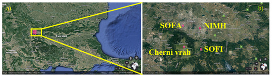
Figure 1.
(a) Map of Bulgaria with indicated locations of observations. (b) Map with a zoom over the Sofia plain. Red markers indicate the stations’ locations and names.
2.1. Objective Circulation Classification: Jenkinson–Collison Type
In this study, objective circulation classification software, Cost733class software v 1.2 (Cost733class v1.2, [26]), was used. The software does a systematic comparison of synoptic classification algorithms and their configuration variants for 12 different European regions. The software package can be downloaded at http://cost733.geo.uni-augsburg.de/ (accessed on 21 April 2023). The Cost733class v1.2 includes over 20 classification methods but, based on a previous study by [25], the Jenkinson–Collison Type (JCT) method was selected. It is a threshold-based classification method with circulation types defined by using a numerical threshold for circulation indices [27]. The main advantage of threshold-based classifications is that they discriminate between synoptically significant types [26]. The assignment of cases is automated by using threshold values for three indices (zonal and meridional flow and vorticity) that result in three states (low, intermediate, and high) and 26 circulation types. To derive JCT circulation types [28], an automated scheme for Lamb weather types [29] is applied to daily 850 hPa geopotential height fields from ERA5 reanalysis [30]. The JCT26 was computed for the domain of southeast Europe with coordinates 7 E–30 E and 34 N–49 N. In Figure 2 the JCT types are presented. JCT circulation classification types are the following: (1) eight directional types, these being West (W), southwest (SW), northWest (NW), north (N), northeast (NE), east (E), southeast (SE) and South (S); (2) Cyclonic (C); (3) AntiCyclonic (AC); (4) eight anticyclonic directional types, these being AW, ASW, ANW, AN, ANE, AE, ASE and AS; and (5) eight cyclonic directional types, these being CW, CSW, CNW, CN, CNE, CE, CSE, and CS.
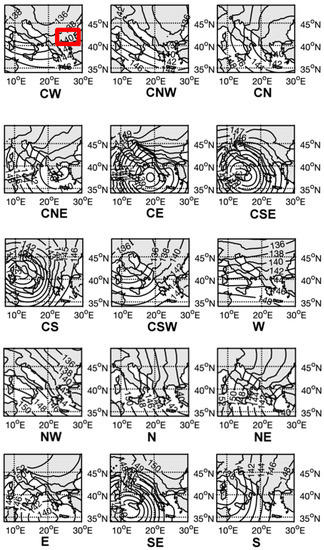
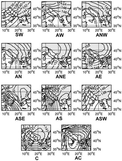
Figure 2.
Map of geopotential heights at 850 hPa for JCT circulation classification with 26 types. For CW type, the position of Bulgaria is shown with a red rectangle.
2.2. SYNOP and ROAB Observations, FSI, SSI
The Fog Stability Index (FSI) is an empirical method for fog forecasting, developed by the US Air Force. It is used in this study in the equation:
where T is the surface temperature in [C], is the dew point temperature in [C], is the temperature at 850 hPa pressure altitude in [C] and is the wind speed at 850 hPa pressure altitude in [m/s]. Fog risk is high for < 31, moderate for 31 ≤ ≤ 55, and very low for > 55 Reymann et al. [31]. We used the as it was originally defined. Although two papers have suggested that the impact of the wind speed on the hit rate is small or negligible, our opinion is that it is still correct to use it in the way suggested by the original definition. The focus of this study was not to improve the FSI or evaluate its components, but to test its skill in detecting fog conditions. Improving the is part of our plans for future study.
In accordance with the study proposed by Stoycheva and Evtimov [32], in Cherni Vrah the Sofia Stability Index (SSI) was applied. The was calculated by using the surface temperatures at Sofia and Cherni Vrah stations in the equation:
where is the temperature of Cherni Vrah (∼2300 m asl.) minus that of Sofia (∼600 m asl.), is the surface air temperature at Cherni Vrah station in [C]. The scaling factor of 17 reflects the altitude difference between Sofia and Cherni Vrah (1700 m), assuming a temperature gradient of 10 C/1000 m.
The index represents an integral characteristic of the degree of stability of the layer between 600 m asl and 2300 m asl, and the approximate altitudes of Sofia and Cherni Vrah. The is based on the Brunt–Väisälä frequency [33] and estimated the strength of the static stability of the airmass over Sofia. A higher value of the Brunt–Väisälä frequency corresponds to a higher degree of stability of the local air mass, with maximum values in the temperature inversion layers.
2.3. GNSS IWV Data Set 2010–2019: SOFA and SOFI
The first GNSS station used in this study is located in Sofia city (SOFA) at an altitude of 667 m asl. The SOFA time-series is available from multipurpose data products of Nevada Geodetic Laboratory (NGL), which processes data from over 17,000 GNSS stations globally [34]. The NGL GPS processing was done with GipsyX v1 software with Precise Point Positioning strategy and the following set up: (1) Jet Propulsion Laboratory GPS orbit products; (2) 7 elevation angle cutoff; (3) 5-min sampling rate. Priori tropospheric models for wet and dry delays were interpolated from the Vienna Mapping Function (VMF1) [35] grid. The mapping function was VMF1. Zenith delay and gradients were estimated with a random walk every 5 min.
The second GNSS station is located on Plana mountain near Sofia (Sofia–Plana, SOFI) at an altitude of 1164 m asl. SOFI is part of the International GNSS Service (IGS) and, in this work, tropospheric products were from the first IGS reprocessing campaign [36,37]. The IGS reprocessing strategy uses the following set up: (1) fixed orbits and clocks; (2) Earth orientation: IGS Final Combined; (3) transmit and receive antenna phase centre map: IGS standards; (4) 7 elevation cut-off angle; (5) GMF hydrostatic and wet mapping function [38]; (6) 24 h data arc; (7) 5 min data rate; (8) estimated parameters: station position, Zenith Wet Delay; (9) delay (3 cm/h random walk), delay gradients (0.3 cm/h random walk) and phase biases (white noise).
The tropospheric product from the GNSS stations SOFA and SOFI are Zenith Total Delay (ZTD). Integrated Water Vapour (IWV) was derived by using surface pressure () and temperature (). The IWV was calculated from ZTD following Davis et al. [39], Bevis et al. [40]:
where [K/hPa], [K/hPa] are constants, first derived by [41] and [J/(kg K)] is the gas constant for water vapour, [K] is the weighted mean atmospheric temperature, h [km] is the height and is the latitude variation of the gravitational acceleration. The pressure difference between the GNSS and SYNOP station altitudes was calculated using the polytropic barometric formula [42]:
where is the pressure at the GNSS station altitude, is the pressure at SYNOP station altitude, T [K] is surface temperature, K/km is tropospheric lapse rate, [km] is the SYNOP station altitude, [km] is the altitude of the GNSS station, m/s is the gravitational acceleration, g/mol is the molar mass of air and N m/(mol K) is the universal gas constant.
2.4. Discriminant Analysis
Discriminant analysis [43] is a well-known technique for classification and assessment of meteorological data. In this paper, analyses were conducted by using Statistica software [44]. All days from November to February of the period 2010–2019 were selected for the statistical analysis. Based on SYNOP data, the 3 hourly registrations were automatically divided into two samples: (1) those with fog registrations (F), including 10 different fog types according to the WMO codes, and (2) those without fog registration (noF), including mist, haze, smoke, dust, drizzle, snow and clear sky. The weather phenomenon reported in the synoptic stations was used in computations [45].
Environmental conditions, i.e. strong stability calculated by the indices SSI and FSI, and IWV data from both groups F and noF were analyzed. The following basic statistics were estimated separately for F and noF groups, and for the IWV from Sofia city and Sofia Plana GNSS stations: median, mean, and 10, 25, 75, and 90 percentiles of FSI, and SSI. An F-test, with a confidence level of 0.05, was applied to determine the statistically significant difference between the groups. Standard discriminant analysis, using Statistica software Sta [44], was applied to obtain the monthly box and whisker plots of FSI and SSI values and their separation into two groups, for F and noF. The following skill scores were calculated:
(1) Probability of detection (POD, [46]):
(2) False Alarm Ratio (FAR, [46]):
(3) Critical Success Index (CSI, [46]):
(4) True Skill Statistic (TSS, [46]):
where is the number of correctly detected F registrations, is the number of incorrectly detected F registrations, is the number of correctly detected noF registrations, and is the number of incorrectly detected/classified noF registrations. POD is the likelihood that a prediction of fog is correct, and FAR is the likelihood that fog is forecast but does not occur. is a measure of the performance of the forecast, although it is not suitable for events with low frequency. also assesses the accuracy.
3. Results
3.1. Circulation Classification: 2010–2019
Fog in Sofia can occur in various atmospheric conditions and it is important to quantify the main circulation types. The objective circulation classification JCT, with 26 types, was computed for a 10-year period for days without fog (noF, blue bars in Figure 3) and for days with fog (F, orange bars in Figure 3). Figure 3 indicates that, on an annual basis, there were the following six circulation types with over 200 noF days: (1) anticyclonic (AC, 546 days), (2) cyclonic (C, 410 days), (3) north (N, 343 days), (4) west (W, 292 days), (5) southwest (SW, 260 days) and (6) northwest (NW, 260 days). The total number of days with fog was only 3% of all thedays in the period. Based on a monthly climatological study conducted by Stoycheva and Evtimov [32], the winter months from November to February have the largest number of fog days in Sofia. As a result, a shorter period was selected, that of November to February for the period 2010–2019, in order to analyze the circulation types leading to fog. Presented in Figure 3b are the circulation types for F and noF days. Six circulation types resulted in fog for the November-February period: (1) anticyclonic (AC) with 18 days of fog, (2) cyclonic (C) with 14, (3) west (W) with 14, (4) southwest (SW) with 12, (5) northwest (NW) with 7, and (6) north (N) with 6. As expected, the AC type had the largest contribution to fog formation as it was associated with clear sky, calm weather, and nocturnal radiation cooling. West and southwest circulation types were responsible for warm air advection, which created conditions for strong temperature inversion. The warm air was usually more humid, but, sometimes, the advection was only at 850 hPa and the airmass at the surface remained unchanged. This happens when the pressure gradient was low and, in these situations, Sofia experiences an almost guaranteed foggy night and morning. The percentages of the fog days for every type are given in Figure 3c. While there were types having even higher fog frequency than the predominant types mentioned above, they were observed very rarely in the 10-year period.
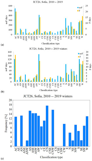
Figure 3.
Number of days with circulation classification JCT with 26 classes for the period 2010–2019. (a) For all months of the year (January–December), (b) only for winter months November–February, and (c) frequency of fog days for every type in the winter months.
In the inner part of the anticyclone, there is very low wind speed or even calm weather, and clear sky. This is caused by the downward airflow in the center of the anticyclone and the divergence towards the rear part of the high-pressure system. Calm weather is responsible for the absence of mixing in the boundary layer, which results in quick saturation caused by enhanced air cooling at the surface and evaporation. The cooling of the air at the surface creates an inversion layer and stable atmosphere stratification which reduces the mixing even further. These conditions during the winter season, when the nights are long and the radiation cooling is strong, make this circulation type most suitable for fog formation. The cyclonic and southwest circulation types result in the advection of warm and humid air masses over Bulgaria, thus facilitating fog formation. For the west circulation type, fog formation is a result of the combination of a weak flow and topography i.e. the high mountains surrounding Sofia city.
3.2. Fog in Sofia 2010–2019: FSI, SSI and IWV
For the period November-February 2010–2019, the FSI monthly box and whisker plots for days with fog registrations (F) and without fog registrations (noF) are computed and presented in Figure 4a. The monthly median FSI values (square in Figure 4a) for F registrations were in the range of 11–21, while for noF registrations they were in the range 31–36. A clear separation between F and noF was also seen for 25 and 75 percentiles (blue and orange boxes in Figure 4a) for every month except February. However, there was an overlap between the 90 percentile of F registrations and the 10 percentile of noF registrations. Comparing this result with the FSI thresholds, it can be concluded that the index has lower values than expected. As can be observed, about 50% of the noF cases had FSI values below the threshold of 31. This was caused either by weather conditions slightly deviating from those necessary for fog formation, or the index required site-specific optimization of its parameters and new thresholds. Nevertheless, the usefulness of the FSI for fog detection in Sofia was confirmed.
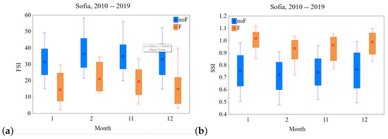
Figure 4.
Monthly box and whisker plots of FSI (a) and SSI (b).
Monthly box and whisker plots of SSI are shown in Figure 4b for the same period. The monthly median SSI had values between 0.9 and 1.0 during fog, while typical SSI monthly median values for noF were around 0.7–0.8. Furthermore, the 25 and 75 percentiles did not overlap. However, the 10 and 90 percentiles did. The threshold value of the SSI used by Stoycheva et al. [19] was 0.98, which was the 22-year mean value for all fog events. As is seen in Figure 4b, a more accurate approach wouold be the usage of monthly thresholds (for example, the medians). The reason behind this was also the different synoptic situations in December and January, compared to November and February. In Bulgaria, fog has a much higher frequency in December and January due to the predominant influence of high-pressure systems. In these two months, the noF distribution had a large spread, especially for December, where the 90 percentile for noF reached the median for F. This can be explained by the fact that the air mass during the anticyclonic type needs a few days for strong enough inversion to form, and for the dew point deficit to be small enough. The SSI as it is defined in Equation (2), does not incorporate the relative humidity and that is why, in Section 3.3, we expand the set of parameters it includes.
It is to be noted that the numbers of fog registrations for February (9) and November (37) were much lower compared to January (88) and December (185), and, therefore, the results for those months may not be reliable.
We further analyzed the GNSS-derived IWV at two stations in Sofia city (SOFA) and the nearby mountain Sofia Plana (SOFI). The results are presented in Figure 5. The monthly box and whisker plots of IWV for F/noF registrations in the period 2010–2019 for SOFA are shown in Figure 5a. On a monthly basis, there was no separation between IWV values for F and noF samples. The fog onset was connected with the transformation of the IWV into cloud droplets. Thus, it was expected that the IWV values would decrease during fog formation and increase during dissipation. A lower spread of IWV values for F cases is clearly seen, compared to noF. This behavior was to be expected because, during fog, there is no change in the air mass and the phase state of water. The bigger spread in IWV values for noF cases was caused by various other (if any) weather phenomena. The absence of separation in the values for F and noF cases can be explained by the 9.5 km distance between the synoptic stations of the NIMH and GNSS stations for SOFA. The NIMH station is located in a lower and more humid area, and most of the time only part of the city is covered by fog. The IWV difference between SOFA and SOFI (Figure 5b) also showed a negligible difference between F and noF cases. This behavior needs further investigation.
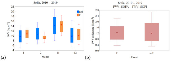
Figure 5.
Monthly box and whisker plots of IWV at: (a) SOFA F/noF sample and (b) difference between SOFA and SOFI for F and noF registrations.
3.3. Probability of Detection and False Alarm for Fog in Sofia
The ultimate goal of this work was to enhance the fog condition detection skills in operational centers in Bulgaria, such as those for public weather and aviation. Therefore, the results are presented in this section for the probability of fog detection using JCT26, FSI, SSI, Wind speed (Wind), Relative Humidity (RH) and IWV. Table 1 presents POD and FAR based on JCT26 (column 2), FSI (column 3) and SSI (column 4). Wind speed (column 5), Relative Humidity (column 6) and IWV from the SOFA station (column 7)are added to SSI. Table 1 shows that the POD, when using daily JCT26 circulation types, was 60.1%. The POD of the FSI, based on 12 UTC observations, was 77.4% and, for the SSI, the POD was computed with a temporal resolution of 3 hours, and was 73.7%. By adding Wind speed and relative humidity to SSI the POD reached 77%. The best result for the POD was 77.9%, obtained by using SSI, Wind speed, RH, and IWV from the station in Sofia city. However, the false alarm ratio remained high in the range of 22% (column 7 line 2). In operational practice in aviation, it is preferred to incorrectly predict fog than to miss it. The low visibility procedures at the airport require tens of minutes to apply and this may result in the inability of an aircraft to land safely. That is why, although the POD was high, the value of FAR was still an issue.

Table 1.
POD, FAR, CSI and TSS using JCT26 (column 2), FSI (column 3), SSI (column 4), SSI and Wind (column 5), SSI, Wind and RH (column 6), SSI, Wind, RH and IWV (SOFA column 7). The period November–February, 2010–2019, was analyzed.
The combination of SSI, wind speed, RH, and IWV results in a function with the equations presented in Table 2. The coefficients were determined for the period 2010–2014 and tested for the period 2015–2019. The results are illustrated in Figure 6. Good skill in fog detection was seen for January and December when most of the fog cases were observed. A threshold value of 19.7 was determined by the mean of the medians for the F cases.
Table 2.
Equations of classification functions based on the following: (1) SSI and Wind, SSI, (2) Wind and RH, and (3) SSI, Wind, RH and IWV. Coefficients were calculated for the period November–February, 2010–2014.
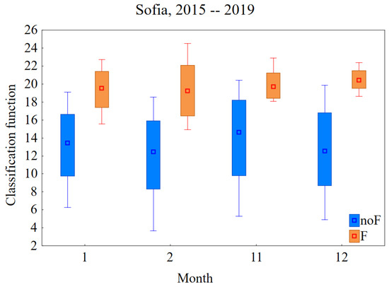
Figure 6.
Monthly box and whisker plots of the classification function F (SSI, Wind, RH, IWV) for F (orange) and noF (blue) cases.
4. Conclusions
Accurate and timely forecasting of the occurrence, development, and dispersion of fog in airport areas is of paramount importance for public weather and aviation meteorological services. Although the proposed index was constructed for a limited area, its effectiveness could be verified in another area, where fog prediction requires additional efforts, accompanied by the involvement of not very complex, but effective, methodologies. The construction of the index, starting from the idea of the physical meaning of the Brunt–Väisälä frequency Stoycheva and Evtimov [32], allows evaluating the state of the atmosphere. Using temperatures at two levels, ground level and at a height slightly above the inversion layer, serves as an indicator of the formation or dissipation of fog. The direct application of the index can be applied in any similar terrain, correcting only for the difference between the two points where the temperature is measured.
In this work, state-of-the-art objective circulation classification was used to quantify the weather types leading to fog in the city of Sofia. While anticyclonic circulation results in the largest number of foggy days in Sofia, there are three other weather types that contribute to fog formation. To the best of our knowledge, these findings are first-of-its-kind and can be of potential interest in operational fog nowcasting. To take into account local factors for fog formation, two fog indices were evaluated. They were found to exhibit good skills in fog detection with a false alarm ratio in the range of 22–26%. No connection was found between the IWV and the fog conditions, but investigating data from future stations, closer to each other, could lead to a change in that result. As a next step, Numerical Weather Prediction proxy profiles of temperature and wind speed will be used to further increase the temporal resolution of the fog indices. A machine learning approach will also be considered.
In summary, it can be concluded that fog forecasting in Sofia can benefit from combining objective circulation classification and locally developed fog indices. However, further improvements in the probability of fog detection and the false alarm ratio are highly desirable. The role of an operational forecaster is indispensable for fog forecasting and nowcasting in the complex terrain surrounding Sofia city.
Author Contributions
Conceptualisation, G.G. and A.S.; methodology, G.G. and A.S.; software, N.P.; validation, N.P.; formal analysis, G.G., A.S., N.P.; writing—original draft preparation, G.G.; writing—review and editing, all authors; visualisation, N.P. All authors have read and agreed to the published version of the manuscript.
Funding
Nikolay Penov and Guergana Guerova acknowledge funding by the European Union-NextGenerationEU, through the National Recovery and Resilience Plan of the Republic of Bulgaria, project No BG-RRP-2.004-0008.
Institutional Review Board Statement
Not applicable.
Informed Consent Statement
Not applicable.
Data Availability Statement
The data is not publicly available.
Acknowledgments
We are very grateful to Piia Post from the Institute of Physics University of Tartu, Estonia, for providing the JCT26 circulation data.
Conflicts of Interest
The authors declare no conflict of interest. The funders had no role in the design of this study; in the collection, analyses, or interpretation of data; in the writing of the manuscript, or in the decision to publish the results.
References
- Steeneveld, G.J.; de Bode, M. Unravelling the relative roles of physical processes in modelling the life cycle of a warm radiation fog. Q. J. R. Meteorol. Soc. 2018, 144, 1539–1554. [Google Scholar] [CrossRef]
- Boutle, I.; Angevine, W.; Bao, J.W.; Bergot, T.; Bhattacharya, R.; Bott, A.; Ducongé, L.; Forbes, R.; Goecke, T.; Grell, E.; et al. Demistify: A large-eddy simulation (LES) and single-column model (SCM) intercomparison of radiation fog. Atmos. Chem. Phys. 2022, 22, 319–333. [Google Scholar] [CrossRef]
- Egli, S.; Thies, B.; Bendix, J. A spatially explicit and temporally highly resolved analysis of variations in fog occurrence over Europe. Q. J. R. Meteorol. Soc. 2019, 145, 1721–1740. [Google Scholar] [CrossRef]
- Boers, R.; Van Weele, M.; Van Meijgaard, E.; Savenije, M.; Siebesma, A.; Bosveld, F.; Stammes, P. Observations and projections of visibility and aerosol optical thickness (1956–2100) in the Netherlands: Impacts of time-varying aerosol composition and hygroscopicity. Environ. Res. Lett. 2015, 10, 015003. [Google Scholar] [CrossRef]
- Vautard, R.; Yiou, P.; Van Oldenborgh, G.J. Decline of fog, mist and haze in Europe over the past 30 years. Nat. Geosci. 2009, 2, 115–119. [Google Scholar] [CrossRef]
- Klemm, O.; Lin, N. What causes observed fog trends: Air quality or climate change? Aerosol Air Qual. Res. 2016, 16, 1131–1142. [Google Scholar] [CrossRef]
- Pérez-Díaz, J.L.; Ivanov, O.; Peshev, Z.; Álvarez-Valenzuela, M.A.; Valiente-Blanco, I.; Evgenieva, T.; Dreischuh, T.; Gueorguiev, O.; Todorov, P.V.; Vaseashta, A. Fogs: Physical basis, characteristic properties, and impacts on the environment and human health. Water 2017, 9, 807. [Google Scholar] [CrossRef]
- Niu, F.; Li, Z.; Li, C.; Lee, K.H.; Wang, M. Increase of wintertime fog in China: Potential impacts of weakening of the Eastern Asian monsoon circulation and increasing aerosol loading. J. Geophys. Res. Atmos. 2010, 115. [Google Scholar] [CrossRef]
- Kampa, M.; Castanas, E. Human health effects of air pollution. Environ. Pollut. 2008, 151, 362–367. [Google Scholar] [CrossRef]
- Dutta, D.; Chaudhuri, S. Nowcasting visibility during wintertime fog over the airport of a metropolis of India: Decision tree algorithm and artificial neural network approach. Nat. Hazards 2015, 75, 1349–1368. [Google Scholar] [CrossRef]
- Hunová, I.; Brabec, M.; Malỳ, M.; Valeriánová, A. Revisiting fog as an important constituent of the atmosphere. Sci. Total Environ. 2018, 636, 1490–1499. [Google Scholar] [CrossRef]
- Izett, J.G.; van de Wiel, B.J.; Baas, P.; Bosveld, F.C. Understanding and reducing false alarms in observational fog prediction. Bound. Layer Meteorol. 2018, 169, 347–372. [Google Scholar] [CrossRef] [PubMed]
- Holtslag, M.C.; Steeneveld, G.J.; Holtslag, A.A. Fog forecasting: “Old fashioned” semi-empirical methods from radio sounding observations versus “modern” numerical models. In Proceedings of the 5th International Conference on Fog, Fog Collection and Dew (FOGDEW2010), Münster, Germany, 25–30 July 2010; pp. 25–30. [Google Scholar]
- Belo-Pereira, M.; Santos, J. A persistent wintertime fog episode at Lisbon airport (Portugal): Performance of ECMWF and AROME models. Meteorol. Appl. 2016, 23, 353–370. [Google Scholar] [CrossRef]
- Song, Y.; Yum, S.S. Development and verification of the fog stability index for Incheon international airport based on the measured fog characteristics. Atmosphere 2013, 23, 443–452. [Google Scholar] [CrossRef]
- Dejmal, K.; Novotny, J. Application of Fog Stability Index for significantly reduced visibility forecasting in the Czech Republic. In Recent Advances in Fluid Mechanics and Heat & Mass Transfer; Wseas: Athens, Greece; Sofia, Bulgaria; Houston, TX, USA, 2011; pp. 317–320. [Google Scholar]
- Lee, J.; Park, J.U.; Cho, J.; Baek, J.; Kim, H.W. A characteristic analysis of fog using GPS-derived integrated water vapour. Meteorol. Appl. 2010, 17, 463–473. [Google Scholar] [CrossRef]
- Stoycheva, A.; Guerova, G. Study of fog in Bulgaria by using the GNSS tropospheric products and large scale dynamic analysis. J. Atmos. Sol. Terr. Phys. 2015, 133, 87–97. [Google Scholar] [CrossRef]
- Stoycheva, A.; Manafov, I.; Vassileva, K.; Guerova, G. Study of persistent fog in Bulgaria with Sofia Stability Index, GNSS tropospheric products and WRF simulations. J. Atmos. Sol. Terr. Phys. 2017, 161, 160–169. [Google Scholar] [CrossRef]
- Alaoui, B.; Bari, D.; Bergot, T.; Ghabbar, Y. Analog Ensemble Forecasting System for Low-Visibility Conditions over the Main Airports of Morocco. Atmosphere 2022, 13, 1704. [Google Scholar] [CrossRef]
- Neykov, N.; Stoycheva, A.; Gospodinov, I.; Gueorguiev, O.; Neychev, P.; Slavov, K. Fog and Horizontal Visibility Forecasting with Stochastic Models. Available online: http://meteorology.meteo.bg/global-change/files/2022/BJMH_2022_V26_N1/BJMH_26_1_1.pdf (accessed on 26 January 2023).
- Kim, S.; Rickard, C.; Hernandez-Vazquez, J.; Fernandez, D. Early Night Fog Prediction Using Liquid Water Content Measurement in the Monterey Bay Area. Atmosphere 2022, 13, 1332. [Google Scholar] [CrossRef]
- Otero, N.; Sillmann, J.; Butler, T. Assessment of an extended version of the Jenkinson–Collison classification on CMIP5 models over Europe. Clim. Dyn. 2018, 50, 1559–1579. [Google Scholar] [CrossRef]
- Voormansik, T.; Müürsepp, T.; Post, P. Climatology of Convective Storms in Estonia from Radar Data and Severe Convective Environments. Remote. Sens. 2021, 13, 2178. [Google Scholar] [CrossRef]
- Stoev, K.; Post, P.; Guerova, G. Synoptic circulation patterns associated with foehn days in Sofia: 1979–2014. IdŐJÁRÁS Q. J. Hung. Meteorol. Serv. 2022, 126, 1–6. [Google Scholar] [CrossRef]
- Philipp, A.; Beck, C.; Huth, R.; Jacobeit, J. Development and comparison of circulation type classifications using the COST 733 dataset and software. Int. J. Climatol. 2016, 36, 2673–2691. [Google Scholar] [CrossRef]
- Post, P.; Truija, V.; Tuulik, J. Circulation weather types and their influence on temperature and precipitation in Estonia. Boreal Environ. Res. 2002, 7, 281–289. [Google Scholar]
- Jenkinson, A.; Collison, F. An initial climatology of gales over the North Sea. Synop. Climatol. Branch Memo. 1977, 62, 18. [Google Scholar]
- Lamb, H.H. British Isles Weather Types and a Register of the Daily Sequence of Circulation Patterns 1861–1971; Meteorological Office: London, UK, 1972.
- Hersbach, H.; Bell, B.; Berrisford, P.; Hirahara, S.; Horányi, A.; Muñoz-Sabater, J.; Nicolas, J.; Peubey, C.; Radu, R.; Schepers, D.; et al. The ERA5 global reanalysis. Q. J. R. Meteorol. Soc. 2020, 146, 1999–2049. [Google Scholar] [CrossRef]
- Reymann, M.; Piasecki, J.; Hosein, F.; Larabee, S.; Williams, G. Meteorological Techniques; Technical Report, AIR WEATHER SERVICE SCOTT AFB IL; John Wiley & Sons Ltd.: Hoboken, NJ, USA, 1998. [Google Scholar]
- Stoycheva, A.; Evtimov, S. Studying the fogs in Sofia with Cherni Vrah-Sofia Stability Index. Bulg. Geophys. J. 2014, 40, 23–32. [Google Scholar]
- Holton, J.R. An introduction to dynamic meteorology. Am. J. Phys. 1973, 41, 752–754. [Google Scholar] [CrossRef]
- Blewitt, G.; Hammond, W.C.; Kreemer, C. Harnessing the GPS data explosion for interdisciplinary science. Eos 2018, 99, 485. [Google Scholar] [CrossRef]
- Boehm, J.; Kouba, J.; Schuh, H. Forecast Vienna Mapping Functions 1 for real-time analysis of space geodetic observations. J. Geod. 2009, 83, 397–401. [Google Scholar] [CrossRef]
- Byun, S.H.; Bar-Sever, Y.E. A new type of troposphere zenith path delay product of the international GNSS service. J. Geod. 2009, 83, 1–7. [Google Scholar] [CrossRef]
- Rebischung, P.; Griffiths, J.; Ray, J.; Schmid, R.; Collilieux, X.; Garayt, B. IGS08: The IGS realization of ITRF2008. GPS Solut. 2012, 16, 483–494. [Google Scholar] [CrossRef]
- Böhm, J.; Niell, A.; Tregoning, P.; Schuh, H. Global Mapping Function (GMF): A new empirical mapping function based on numerical weather model data. Geophys. Res. Lett. 2006, 33. [Google Scholar] [CrossRef]
- Davis, J.; Herring, T.; Shapiro, I.; Rogers, A.; Elgered, G. Geodesy by radio interferometry: Effects of atmospheric modeling errors on estimates of baseline length. Radio Sci. 1985, 20, 1593–1607. [Google Scholar] [CrossRef]
- Bevis, M.; Businger, S.; Herring, T.A.; Rocken, C.; Anthes, R.A.; Ware, R.H. GPS Meteorology: Remote Sensing of Atmospheric Water Vapour Using the Global Positioning System. J. Geophys. Res. 1992, 97, 15787–15801. [Google Scholar] [CrossRef]
- Thayer, G.D. An improved equation for the radio refractive index of air. Radio Sci. 1974, 9, 803–807. [Google Scholar] [CrossRef]
- Sissenwine, N.; Dubin, M.; Wexler, H. The U.S. Standard Atmosphere, 1962. J. Geophys. Res. 1962, 67, 3627–3630. [Google Scholar] [CrossRef]
- Huberty, C.J. Discriminant analysis. Rev. Educ. Res. 1975, 45, 543–598. [Google Scholar] [CrossRef]
- StatSoft Inc. STATISTICA (Data Analysis Software System), 6th ed.; StatSoft Inc.: Tulsa, OK, USA, 2001; p. 150. Available online: www.statsoft.com (accessed on 26 January 2023).
- WMO. Manual on Codes. 2019. Available online: https://library.wmo.int/doc_num.php?explnum_id=10235 (accessed on 27 December 2022).
- Hanssen, A.; Kuipers, W. On the Relationship between the Frequency of Rain and Various Meteorological Parameters. (With Reference to the Problem of Objective Forecasting); Koninklijk Nederlands Meteorologisch Instituut: Hague, The Netherlands, 1965.


Disclaimer/Publisher’s Note: The statements, opinions and data contained in all publications are solely those of the individual author(s) and contributor(s) and not of MDPI and/or the editor(s). MDPI and/or the editor(s) disclaim responsibility for any injury to people or property resulting from any ideas, methods, instructions or products referred to in the content. |
© 2023 by the authors. Licensee MDPI, Basel, Switzerland. This article is an open access article distributed under the terms and conditions of the Creative Commons Attribution (CC BY) license (https://creativecommons.org/licenses/by/4.0/).