Abstract
Due to its important spatiotemporal variability, accurate rainfall monitoring is one of the most difficult issues in semi-arid mountainous environments. Moreover, due to the inconsistent distribution of gauge measurement, the availability of precipitation data is not always secured and totally reliable at the instantaneous time step. As a result, earth observation of precipitation estimations could be an alternative for overcoming this restriction. The current study presents a framework for either the hydro-statistical evaluation and bias correction of the Global Precipitation Measurement (GPM) Integrated Multi-SatellitE Retrievals version 06 Early (IMERG-E), Late (IMERG-L), and Final (IMERG-F) products. On a sub-daily duration, from the Taferiat rain gauge-based station, which was used as a benchmark from 1 September 2014 to 31 August 2018. Statistical analysis was performed to examine each precipitation product’s performance. The results showed that all Post_Real_Time and Real_Time IMERG had a high level of awareness accuracy. The IMERG-L results were statistically similar to the gauge data, succeeded by the IMERG-F and IMERG-E. The Cumulative Distribution Function (CDF) has been employed to adjust the precipitation values of the three IMERG products in order to decrease bias estimation. The three products were then integrated into the “HEC-HMS” hydrological model to assess their dependability in flow modeling. Six flood occurrences were calibrated and validated for each product at 30-minute time steps. With a mean Nash-Sutcliffe coefficient of NSE 0.82, the calibration findings demonstrate that IMERG-F provides satisfactory hydrological performance. With an NSE = 0.80, IMERG-L displayed good hydrological utility, slightly better than IMERG-E with an NSE = 0.77. However, when the flood events were validated using the initial soil conditions, IMERG F and IMERG E overestimated the discharge by 13% and 10%, respectively. While IMERG L passed the validation phase with an average score of NSE = 0.69.
1. Introduction
The global hydrological cycle and atmospheric energy exchange are highly dependent on precipitation [1,2]. Understanding the spatiotemporal variability and accuracy of rainfall information is critical for numerous utilizations such as hydrological modeling, climate forecasting and water management [3,4,5].
Indeed, Extreme flows pose a significant threat as a natural hazard, often resulting in considerable property damage, as demonstrated by the Oued Ourika flood disaster of 17 August 1995 [6].
Furthermore, the lack of suitable rainfall measurement stations is an extremely critical challenge, particularly in Mediterranean regions marked by a hilly and steep slope, sparse, inconsistent, and often accompanied by low-measurement-quality data [7,8,9,10,11,12,13,14], where rain gauges (RG) data are generally used as a reference. Indeed, the network density in Mediterranean Africa has declined significantly over years [15,16]. As a result, assessing and forecasting precipitation occurrences over these areas remains difficult. Ground observations, radar measurements, and satellite estimates are the three main methodologies and devices for measuring precipitation [17]. In fact, a sparse network, significant missing readings, wind disturbances, and a scarcity of stations significantly impact precipitation gauges [18]. Additionally, signal attenuation, surface backscatter, and uncertainty issues with the reflectivity-rainfall-runoff ratio affect ground-based radar observations [19].
Furthermore, satellite precipitation products (SPP) have been the main method for quantifying precipitation in recent decades [19,20]. It may provide the most precise and robust approach to quantifying worldwide precipitation due to their large spatial distribution and continuous tracking [21,22,23]. The Tropical Rainfall Measurement Mission (TRMM) [22] and the Global Precipitation Measurement Mission (GPM) [24] highlight two key stages in the evolution of Satellite Precipitation Products (SPP). These SPP commonly generate global precipitation observations on high spatial and temporal scales. Laded by the National Aeronautics and Space Administration (NASA) and the Japan Aerospace Exploration Agency (JAXA), the GPM is an international mission, as a continuation and enhancement of the TRMM satellite observations of global precipitation and snowfall [22,25,26]. IMERG, TRMM’s worldwide successor provides more accurate spatiotemporal scales (30-min intervals, and 0.1°-0.1°) and global precipitation estimates with quasi-worldwide coverage (60°N–60°S) [27] including three products with varying latencies: the near-real-time Early and Late (IMERG-E and IMERG-L), as well as the post-real-time “Final” (IMERG-F) [27,28]. The three IMERG produces are called “Early, Late, and Final runs” because of their latency.
Numerous studies have been conducted to compare IMERG precipitation to measurements such as radar and ground-based gauges, as well as to other available earth observations of precipitation data (e.g., [15,21,29,30,31,32,33,34]). As a result, reliable real-time SPP with high spatiotemporal resolution are critical for hydrological models to offer accurate flood forecasts [35]. However, SPP are vulnerable to a range type of errors [36,37], including sensor errors [38], and retrieval algorithms [39,40]. However, SPP errors are caused by two factors: (1) random error, which is inherent in the measurement records, and (2) systematic bias, which is related to the post-processing algorithms and procedures used to assimilate the available data over a specific region for a specific time. Nevertheless, systematic bias can be reduced or eliminated by applying statistical bias correction methods to SPP. Several bias correction methods have been developed to improve SPP products, ranging from commonly used simple scaling approaches to advanced distribution mapping [41]. However, in this paper, the ground-based data of the Cumulative Distribution Function (CDF) were obtained by applying a distribution mapping method that considers only the recorded rainfall data. The Quantile mapping (QM) approach has already been successfully implemented not only for the correction of the SPP bias [42,43,44], but it has also been utilized to correct general circulation model bias [45,46]. Furthermore, the GPM products IMERG V 06 IMERG_E, IMERG_L, and IMERG_F were chosen since they are recommended for extreme event applications [47]. These data have first undergone a comprehensive statistical analysis, then a bias correction at sub-daily time steps (30 min).
Following by the identification of rainfall events, which were simulated, calibrated, and validated in a hydrological model using data from the Taferiat rain gauge between 2014 and 2018. Since limited work has been devoted to statistical and hydrological assessments of the GPM IMERG V06 product, this study will highlight the mismatches between earth observation and gauge precipitations. The purpose of this paper is to statistically analyze the IMERG V06 products with gauge precipitation. To validate the implementation of the used products in the hydrological modeling of extremes across complex topography, and identify products that can estimate well-simulated precipitation and runoff in semi-arid mountainous regions.
The following paper is structured as follows: Section 2: Description of the study area and presentation of the used precipitation data sets. Section 3: Assessment of the spatial distribution of rainfall and its impact on surface water at the outlet. Then, employing the QM method and the CDF function, the processing of data and bias correction of the SPP are performed. Section 4: Calibration by forcing the HEC-HMS model with IMERG precipitation data and comparing it with the rain gauge data, in order to determine its capacity to detect different precipitation events, and to reproduce extreme flows. Finally, Section 5: contains findings and suggestions for upcoming work. This section provides the first comprehensive analysis of the viability of SPP in the modern era. The results should provide researchers with useful information on the performance of the various runs, to validate the suitability of the newest IMERG V06 version as a source of rainfall data for forecasting and providing early warning of potential hazards as extreme precipitation events in the Mediterranean mountainous zones.
2. Research Location and Used Data
2.1. Study Area
The study area is the Zat catchment, a tributary of the Tensift river basin. It is located in the South EST of Marrakech city with latitudes 31°30 and 31°45 north and longitudes 7°30 and 7°45 west, as shown in Figure 1. With elevations ranging from 756 to 3777 m and a surface of 521 km2 [7], while the annual precipitation average is 395 mm, of which 30% is snow at altitudes above 2000 m [48,49], the climate is intermediate between semiarid and humid in the upstream, semi-arid in the downstream, and greatly impacted by altitude [50]. The Zat catchment is characterized by a complex river network, recognized by a dense and complicated hydrographic network. A river drains the Zat Basin and connects with the Ourika River to form the Hadjar River’s two main tributaries. The upstream geology is defined by the outcrop of Precambrian terminal igneous and metamorphic rocks and is considered impermeable. While the downstream is in the northern sub-Atlantic zone, the principal outcrops are from the post-Hercynian layer mostly permeable [51]. At the highest elevations, the slope’s average is 19% [52]. These environmental conditions encourage the creation of runoff. The vegetation is divided into two sections: the forests in the mountain area upstream and the agricultural section downstream, which includes cultivated land along the river channel.
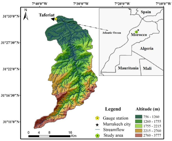
Figure 1.
Situation of the Zat basin, the topographic elevation, the river network and the location of the Taferiat gauging station.
2.2. Gauge Precipitation Data
Precipitation varies considerably in space and time, especially in mountain basins. Ground observations are used to analyze precipitation and runoff, as well as a reference for rainfall data since it provides a continuous record in a specific location. Within this study, we used the 10-min sub-daily precipitation from the Taferiat station, upscaled to 30 min to match the satellite precipitation (Figure 1), the Tensift Hydrological Agency (ABHT) supplied these observations. Although rainfall in the Zat basin is very low and there is only one station downstream. Data collection was based on the availability of rainfall records from 1 September 2014 to 31 August 2018. All recorded data were subjected to rigorous quality control, which includes checking for outliers and nulls with a variety of approaches such as the “letter-value” approach of the python package “seaborn” and hoarding curves. This ensures that the ground-based rain gauge data is of excellent quality. This in situ data collection was exploited as a baseline to validate the used IMERG products.
2.3. Earth Observation of Precipitation Data
The GPM project is a joint collaboration between NASA and JAXA. GPM provides three distinct data treating levels. It includes gridded precipitation and snowfall data at a spatial resolution of 0.1° × 0.1° at a 30-min frequency [53], based on a combination of PMW and IR data from GPM and gauge analysis by the GPCC. The principal modifications in the recent IMERG release are (1) the inclusion of SAPHIR and the IMT estimates; (2) Passive microwave estimation are altered at high latitudes to decrease spatial gaps; (3) the inclusion of GEOS, FP, and MERRA-2 model data for time interpolation in place of the IMERG V05 infrared data [54].
The IMERG system will run two instantaneous runs, once to generate IMERG-E at about 4 h after the rated observing time, then to generate IMERG-L data with about 12 h latency, and after receiving the monthly level analysis, the last IMERG run will be run to generate IMERG-F data at about 3.5 months. The IMERG run (NRT) uses the climatological observations from the gauges for bias adjustment, it also uses the monthly analyses from the GPCC gauges [54].
In this study, temporal, statistical, and hydrological analyses were performed to determine the ability of the GPM to identify significant rainfall events that occurred between 1 September 2014 and 31 August 2018.
2.4. Discharge Data
Flow data from the Taferiat gauging station was used for calibration and validation of the HEC-HMS model. The Tensift hydrological agency (ABHT) provided the flow data from 2014 to 2018. Throughout these four years, only six flash floods were triggered by heavy rains, the details are presented in Table 1.

Table 1.
Specifications of flash floods events.
When analyzing these flood events, the following points should be highlighted: Event 1 has not been calibrated or validated due to a lack of precipitation data, Event 3 has a higher peak discharge value than the other events and has a Multi-modal temporal distribution, whereas the other events have a Uni-modal distribution. Furthermore, event 4 has a significantly lower maximum drain than the other events. It should be emphasized that precipitation has a significant impact on flood events.
2.5. HEC-HMS Software
HEC-HMS is a deterministic, semi-distributed, event-based/continuous, and mathematically based model. It is able to model in a wide variety of geographical regions, and different climatic contexts, such as arid and semi-arid mountainous climates [15]. It easily conducts a wide range of hydrological study functions, such as losses, discharge transformation, routing in open channels and analysis of meteorological data, simulation of precipitation and runoff, and estimation of parameters [55].
3. Methods
3.1. Processing Data
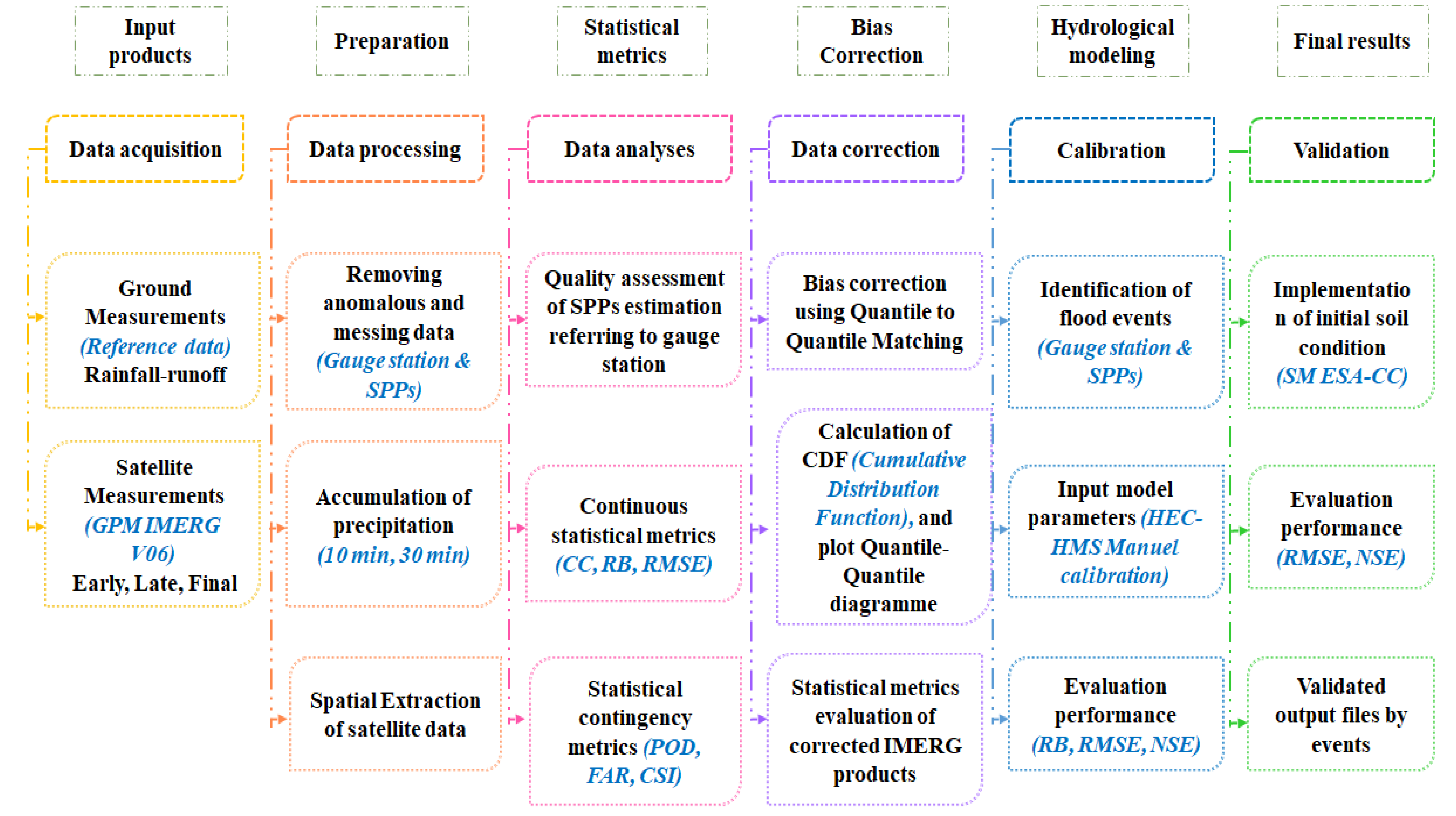
To evaluate the IMERG products, satellite and gauge precipitation data were pre-processed to ensure data consistency and accuracy. This involved several actions (Figure 2): (1) Examine the continuity of the rain gauge and IMERG data. (2) Remove outliers and missing data to ensure symmetry. (3) upscaling the rain gauge data from 10 min to 30 min to match the satellite data. (4) Compare the satellite data from the GPM IMERG V06 products with the rain gauge data (taking into account the average precipitation pixels that are closely correlated with runoff). (5) Computation of statistical metrics, and bias correction using the CDF function. (6) Finally, hydrological modeling using the HEC-HMS hydrological model by using observed and satellite data.

Figure 2.
Diagrammatic of the evaluation process for this study.
For this purpose, two scenarios were carried out. The first scenario concerns the calibration with the forcing of the model with observed and satellite rainfall data, whilst the second scenario concerns the validation using the “leave-one-out” method based on the initial soil moisture conditions extracted from ESA-CCI satellite data with the calibrated curve number. (More details in Section 4.4).
3.2. Satellite Monitoring of Precipitation Products
Satellite precipitation data from the IMERG product were downloaded from Net-CDF grid files from 1 September 2014 to 31 August 2018. Data visualization with an extraction tool was applied to extract gridded precipitation from the Net-CDF files [56]. In addition, various metrics including average, variation coefficient, and standard deviation were used to assess the overall performance of the earth observation rainfall products. This provides insight into the outcomes of the remotely sensed precipitation estimations selected for the research area. A method for analyzing the effect of precipitation on streamflow in each pixel of the research area was developed. Section 4.1 Precipitation spatialization and runoff evaluation in the findings section discusses the detailed method better.
3.3. Metrics Assessment
Multiple analytical methods have been used to quantify the quality of the three SPPs in comparison to in situ precipitation and to investigate the adequacy of the IMERG products. Statistical metrics including, Root Mean Square Error (RMSE), Pearson Correlation Coefficient (CC), Bias, Mean Squared Error (MSE), The Mean Absolute Error (MAE), are utilized to represent the agreement and uncertainties between the IMERG products and the gauge measurements. The purpose of the CC is to assess the amount of linear connection between the IMERG data and the measurements. CC value can range from −1 to 1, with 0 representing no correlation.
Root Mean Squared Error (RMSE) is a commonly used metric to evaluate the performance of regression models. It is the square root of the Mean Squared Error (MSE) and measures the average magnitude of the differences between the predicted and actual target values. Where a lower value indicates an excellent quality assessment. Note that positive Bias numbers denote an over-estimate and negative numbers an under-estimate. IMERG products are commonly considered credible if the CC value is superior to 0.7 and the Bias value ± 10% [57]. The Mean Squared Error (MSE) is a commonly used loss function for regression problems, is widely used as a performance metric for regression models, and is used to minimize the difference between the predicted values and the actual values. The Mean Absolute Error (MAE), is defined as the average of the absolute differences between the predicted values and the actual values.
The diagnostic indices are as follows:
where N represents the number of samples; are gauge observations and their average; represent satellite estimates and their average, respectively.
Three contingency metrics have been used to assess the ability of precipitation detection capability of IMERG namely POD, FAR and CSI. To differentiate precipitation days and days without precipitation, a threshold value of 0.1 mm/h was chosen.
The fraction of SPPs that correctly recognize the precipitation recorded in the measurement gauges are measured by POD. FAR stands for the percentage of SPPs that detect rainfall events that are not detected by measurement stations. The former approach compensates for random events, while the latter describes the correspondence between the days of precipitation recorded by the PPSs and the levels. POD = 1, CSI = 1, and FAR = 0 for a perfect score. Examples of categorical statistical measures include:
with H as the precipitation event recorded by the satellite and ground station at the same time, M as the rainfall event recorded by the rain station but excluding the earth observation, and F as the inverse of M. The calculus of the CSI includes the identification of a threshold of rain/no rain events. In this study, the time resolution of the rain gauge and SPP is 30 min. The rainfall threshold was set at 0.1 mm/30 min.
3.4. Quantile Mapping Method
Using a non-parametric method, such as the QM method, the Empirical Cumulative Distribution Function (ECDF) of earth precipitation observations can be fitted to match the (ECDF) of gauge estimations using a transfer function for each quantile [58].
This strategy has already demonstrated promising results in removing systematic biases from climate models whose resolution is too rough to be explained the great variability of precipitation patterns. Similarly, satellite products from a certain time period are modified to account for the statistical features of precipitation records [59,60,61]. Wilks, 2011 [62] detailed the method for generating ECDFs, and Themeßl, 2012 [63] used it for Quantile Mapping (QM) precipitation from climate models.
ECDFs are calculated for all SPPs in this study. The matching process used here can be mathematically represented as follows:
where PIMERG-Cor is the corrected rainfall quantity, PIMERG is the rainfall quantity to be corrected, ECDF-1G represents the equivalent of the empirical CDF of the rain station data, and ECDF Gauge is the empirical CDF of the gauge precipitation. Each percentile of the IMERG precipitation series is substituted by a percentile of the rain gauge precipitation data-series in this approach.
In other words, for the pixels in the Zat basin, the probability of surpassing the SPPs precipitation quantity is computed using the empirical CDF generated from the SPPs. The empirical CDF from the in-situ observation is then utilized to calculate the probability of precipitation. The sub-daily precipitation quantity for the most representative pixels of the Zat basin (P2, P5, P6, P7, P9, and P11) are adjusted through this CDF matching technique based on the ECDF generated for the SPPs and ground data for the analyzed basin.
This approach not only adjusts themes and standardizes their deviance, but it also keeps each quantile magnitude from observations, including those from the distribution’s higher tail [63].
3.5. Hydrological Process
The IMERG products were hydrologically evaluated using the HEC-HMS model version 4.9. The Digital Elevation Model (DEM) was incorporated into the HEC-Geo-HMS Extension tool in the Arc GIS. The established simulations were in 30-min time-steps. Indeed, eight parameters were calibrated manually by maintaining the maximum and minimum ranges based on the literature [64], which are: (1) Initial Abstraction (mm), Curve Number (CN), and Impervious (%), for the Loss method. (2) Then, Time of concentration (HR), and Storage Coefficient (HR) for the Transform method. (3) Finally, Initial discharge (m3/s), Constant recession, and Ratio for the Baseflow method. Table 2 lists the parameters and methodologies used in watershed modeling.

Table 2.
Selected methods for the HEC-HMS model [65].
The used Methods incorporate SCS-CN (Soil Conservation Service) Curve Numbers, Clarke Unit Hydrographs, and Base Flow Recession required to establish the hydrologic loss rates, runoff transformation, and base flow [7,65,66,67,68,69,70].
After completion of the model calibration, IMERG products were validated using the initial soil conditions, and the soil moisture from the ESA-CCI database for each flood occurrence throughout the study period. Indeed, the ESA-CCI soil moisture product, provided by the European Space Agency (ESA) (http://www.esa-soilmoisturecci.org/) (accessed on 2 February 2023), gives estimates of SM on the day(s) preceding a flood event considered as the initial soil condition, which gives an idea of the soil saturation rate and therefore an idea of flood occurrence probability. The product has a temporal sampling of 1 day and a spatial resolution of 0.25°. However, the implementation of the SM (from ESA-CCI) in the model was developed by applying a linear regression between the initial satellite soil moisture for each event and the CNs obtained after the calibration of each event. New CNh were derived from the linear equation relating the soil moisture data to the calibrated CNs using a re-sampling approach without reinsertion. The model was then forced by the newly obtained CNh, at the validation level. This method has already been validated in the High Atlas watersheds.
In addition, IMERG products were incorporated into the HEC-HMS model by replacing precipitation from the gauge with IMERG data. The Nash-Sutcliffe coefficient NSE, PBIAS, and RMSE have been utilized to assess the model to estimate the “ quality of fit “ of the observed and estimated flows.
Furthermore, NSE is a commonly used metric for evaluating the performance of hydrologic models and is based on the comparison of simulated and observed flow values. In our case, the HEC-HMS model privileges the calculation of NSE, RMSE, and PBIAS directly at the platform level. This leads us to take into account the NSE rather than other metrics.
The performance of the HEC-HMS model is compared to the literature using the following criteria:
The Nash-Sutcliffe Coefficient (NSE) ranges from −∞ to 1, with negative values indicating poor performance [68] classifies model performance into 4 categories: (1) inadequate (NSE 0.5); (2) satisfactory (NSE > 0.5); (3) good (NSE > 0.7); and (4) extremely good (NSE > 0.8). It can be used to assess the model’s predictive power and is computed as follows:
The PBIAS is for assessing the average tendency of observed flow to simulated flow difference [68]. It is formulated as follows:
The RMSE for calculating the residuals between simulated and observed runoff values [68]. RMSE is expressed mathematically as follows:
where is the data being evaluated, is the simulated data, is the mean of observed data and n is the total number of observations.
3.6. DEM
Terrain preprocessing begins with the preparation of a Digital Elevation Model (DEM). It is tiled with a resolution of about 30 m. Downloaded from the United States Geological Survey (USGS).
This DEM was cropped along watershed boundaries using county polygon shapefiles downloaded from ESRI (Figure 1).
4. Results
4.1. Rainfall Spatialization and Runoff Assessment
Precipitation and runoff have important spatiotemporal characteristics, especially in semi-arid mountainous areas. Therefore, an approach to analyzing the influence of precipitation falling in each pixel on streamflow patterns in the outlet of the basin has been developed. The Zat watershed was classed into 15 pixels of 0.1° × 0.1°, which is the resolution of the satellite pixels. The grid of pixels was analyzed by applying a series of evaluation metrics which are Pearson’s Correlation Coefficient, and Root Mean Squared Error, to identify the pixels having the greatest influence on watershed flow. The six most representative pixels, which occupy a volume higher than 60% of the total pixel area, and whose correlation coefficients are satisfactory (P2, P5, P6, P7, P9, and P11) as shown in Figure 3, with correlation coefficients of 0.5, 0.48, 0.73, 0.52, 0.94, and 0.67, respectively.
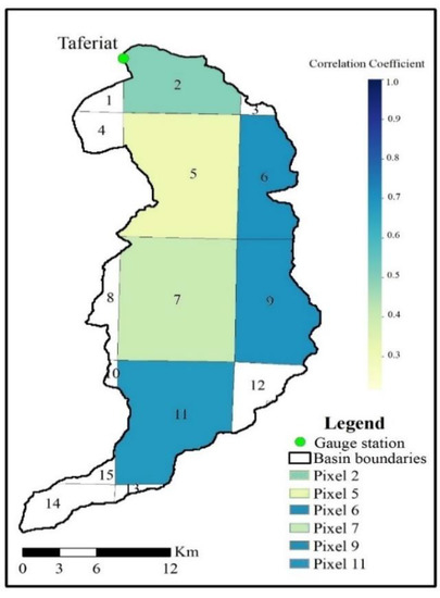
Figure 3.
Spatial IMERG rainfall variability and its influence on runoff in the outlet.
Subsequently, a regression of multiple linear approaches has been applied for each pixel in the three products, which has confirmed the previous results of the representative pixels, noting that each pixel is defined by representing the volume of precipitation falling on each pixel, which is shown in the equations below (Equations (13)–(15)). Multi-linear regression factors are based on the relationship between multiple variables and are calculated by examining the correlation between them. The calculation of multi-regression factors can vary depending on the data set. In our case, different precipitation products (early, late, and final) were used to build the multi linear regression, which gives different factors.
P(1,3,4,8,10,12,13,14,15) are removed from equations 11,12, and 13, because the calculated factors multiplying these pixels are equal to zero, therefore, their impact on the equation is eliminated. This means that the equation will no longer be affected by these values and any changes in them will have no effect on its result.
In addition, each pixel is multiplied with a factor linked to the volume of precipitation and its distance from the measuring station. The resulting equations can be used to forecast the average flows directly from IMERG precipitation data.
4.2. Performance of CDF Matching Method
Based on previous research, such as [58,69], the CDF approach performs well. This produced the most accurate representations and was less susceptible to inaccurate adjustment of isolated anomalies in locations where the gauge is sparse, as is the case in our situation. Although the data sets may be quite different locally, their relative frequency may be similar, limiting the vulnerability to excessive fitting mistakes. The gamma distribution may not be acceptable at dry locations with many zero totals, since zero values must be removed in the adjustment. Indeed, with a larger data set, this approach will almost certainly be more effective, for providing only 4 years’ worth of data may limit the strength of the goodness-of-fit, particularly for the extremes. For example, in the [44], they improved the quantity of available data for fitting using daily observations and taking into account the adjacent grid cells, which have a tendency to improve the precision of this technique.
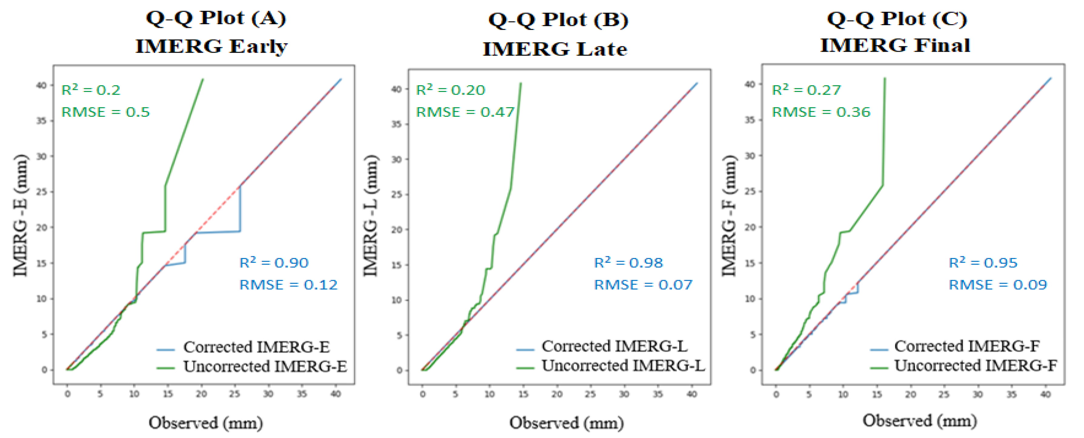
The CDF technique, on the other hand, does not depend on gauge analysis to provide accurate totals, but rather on the more accurate gauge frequency. Indeed, the representation is comparable to that obtained by linear correction models. The CDF matching approach is a simple algorithm, but it can be effective in some situations. It may be useful in locations where rain gauge networks are more sparse and accurate analysis of rain gauges is more difficult, as is the case in the study watershed. Figure 4 shows a comparison of 30 min SPPs during the whole study period using Quantile-Quantile (Q-Q plots). The precipitation Q-Q plots demonstrate reasonable bias-corrected performance relative to observations, with data lines extremely close to the baseline for both the Late and Final runs. The Q-Q graphs show that the corrected satellite precipitation products have a decent ability to reduce bias in general.
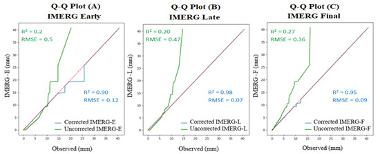
Figure 4.
Q-Q plots comparing IMERG precipitation products with and without correction using the CDF function for (A) IMERG Early, (B) IMERG Late and (C) IMERG Final products. The 1:1 line is presented in red Dash line.
The results reveal that following bias reduction using the CDF matching method, all data products (Figure 4, particularly IMERG_L and IMERG_F), (Figure 4B,C) improved significantly. While the IMERG_E data indicated a slight improvement, (Figure 4A). As a result, the QM technique results indicated that the IMERG_E data may have higher uncertainty than the IMERG_L and IMERG_F data.
4.3. Statistical Indices Assessment
In order to emphasize the significance of bias correction for remotely sensed precipitation, a statistical comparison was conducted between bias-corrected and uncorrected (IMERG_E), (IMERG_L), and (IMERG_F) products and ground-based precipitation data at the Taferiat station for six typical pixels in the Zat Basin. The study period was from 1 September 2014 to 31 August 2018.
The statistical assessment results at sub-daily (30 min) time steps are shown in Table 3. Indeed, near-real-time products IMERG_E and IMERG_L achieved comparable Correlation coefficient (CC) values that were somewhat lower compared to IMERG_F and statistically insignificant before adjustment. In contrast, after bias corrections for all SPP, the (CC) values between ground-based precipitation observations and the SPP improved dramatically and became statistically significant. The major cause is because of the SPP algorithm, short-term SPP estimates typically include significant biases, and aggregation of SPP from thinner to coarser time step resolutions could partially compensate for precipitation bias in the finer time steps, resulting in increased (CC) in the longer time steps. However, precipitation was significantly underestimated in IMERG_E and IMERG_L and slightly overestimated in IMERG_F before bias corrections. In addition, although IMERG_L outperformed IMERG_F and IMERG_E in general, a small margin of error was noted. Table 3 reveals that IMERG_L had marginally lower RMSE values by comparing it to IMERG_E and IMERG_F before correction, but the resultant RMSEs are significant after correction. This result suggests that the IMERG SPP contain a number of outliers. Based on Bias, IMERG_E and IMERG_L significantly overestimated precipitation before corrections by 23.53% and 15.83%, respectively, while IMERG_F attained a significantly lesser systematic Bias (6.87%) due to the in-situ adjustment using precipitation on a monthly basis from the Global Precipitation Climatology Centre (GPCC) gauge analysis, while the obtained Bias is significantly improved and significant after corrections. Moreover, the Mean Square Error (MSE) and the Mean Absolute Error (MAE) represent values between 0.17 and 0.23 and 0.40 and 0.60, respectively, before corrections, and between 0.13 and 0.19 and 0.04 and 0.06, respectively, after corrections, which shows a clear improvement of the results after corrections.

Table 3.
Summarized statistical descriptive of rainfall estimates from the (GPM) earth observation at the sub-daily scale.
Regarding the ability of SPP to detect rainfall events, IMERG’s three SPP performed similarly, with PODs and CSIs ranging from (0.18 and 0.28) and (0.06 and 0.09), respectively, before correction, and from (0.93 and 0.99) and (0.94 and 0.97), respectively, after correction, indicating a significant improvement. FAR readings below 0.90 before rectification, followed by an astonishing improvement with values extremely close to the optimal 0. In all criteria, the IMERG_L outperformed the IMERG_E real-time product and the IMERG_F post-real-time product.
4.4. Hydrological Calibration and Validation
In terms of calibration and validation, rainfall events have been chosen depending on the disposal of data records of discharge and precipitation for the most extreme events that have occurred recently. The selected rainfall events in Table 1 are used for calibration and validation. Both processes have been done manually using data from the Taferiat measuring station at 30 min time step for the period from 2014 to 2018.
The events studied in this research were classified based on their point flow into three categories: Heavy flash flood, which has a flow of ≥50 m3/s, Moderate flash flood, with a flow of ≥20 m3/s, and Low flash flood, which has a flow of ≥10 m3/s. Events 1 and 3, which occurred during summer and autumn, had a peak flow (Q max) of 66.82 m3/s and 136.61 m3/s, respectively, ranking them as heavy flash flood events. On the other hand, Events 2, 5, and 6 took place between autumn and spring, which is the peak season for flash floods in the region, with peak flows of 34.30 m3/s, 38.86 m3/s, and 21.74 m3/s, respectively, classifying them as moderate flash floods. Event 4 was a small spring flood event that resulted from snowmelt, with a peak flow of 12.13 m3/s, which was categorized as a low flash flood event.
Calibration process: A total of 24 events were simulated and calibrated using the initial values. However, the calibration was developed by maintaining the maximum and minimum ranges of the calibration parameters based on the literature [7,15]. The averages of these intervals were considered as initial values in the case of this paper. These values were manually adjusted to obtain a good fit within the observed and estimated flows. The quality of the adjustment was judged using the visualization of the hydrographs and the calculated statistical values. However, a critical analysis was applied to ensure that the input parameter values used are physically meaningful by evaluating the watershed and stream characteristics.
Table 4 represents the calibration parameters of the 24 events studied which are:

Table 4.
Calibration parameters of the hydrological model.
1—Curve number (CN): mainly depends on the land use land cover maps (LULC), and soil maps. It could be calculated using GIS methods. However, in this study, the CN was calculated using the weighted average of the total number of curves in the Zat basin and resulted in an average value of CN = 72.
2—“Time of concentration”: defined as the time required by water to flow from the farthest point in the watershed to the outlet side. It was calculated using the Giandotti equation as below:
where: Tc is the Time of concentration in (Km/√m), S is the basin area in (Km2), L is the length of the main stream (Km); H avg is the average altitude (m), and H min is the minimum altitude (m).
3—“Recession constant”: describes the rate of baseflow decay, the constant represents the ratio of the baseflow at the present time to the flow one day earlier and is therefore between 0 and 1. The actual value would be further defined in the hydrologic modeling process, looking for the value that gives the best efficiency.
Validation Process: is used to verify the model’s accuracy in this study was performed using multiple approaches due to the limited size of the identified and studied flood events. Specifically, the “leave-one-out” resampling method was employed in this paper, whereby each of the n flood events (i) was removed in turn. By doing so, the relationship between the root and soil moisture measured using a time domain reflectometry tool (TDR) and the two models’ most sensitive calibration parameters (curve number (CN) and time of concentration (TC)) could be established.
The calculated CN values obtained by this procedure are then used to model flood event and the simulated flow is compared to the observed flow. The validation results for the 24 events are presented in Table 5, indicating better model performance when using the SCS-CN model and accounting for soil moisture, with Nash coefficients between 0.47 and 0.90, using the leave-one-out procedure [15]. This approach is a good alternative for hydrological modeling in poorly gauged or ungauged basins [15].

Table 5.
Hydrological model validation parameters.
In addition, all hydrographs from the three products have been compared based on several statistical indicators, involving flood volume, maximum floods, NSE, PBIAS, and RMSE, which are significant performance metrics in event-based modeling Table 4 and Table 5.
In general, results demonstrate a close agreement between the observed and estimated flow at the peak flow values and a reasonable agreement in terms of discharge distribution. In addition, the evaluation criteria show satisfactory values for the NSE, which is between 0.6 and 0.91 for the calibration, and 0.47 and 0.90 for the validation.
4.4.1. Calibration and Validation of IMERG Early Events
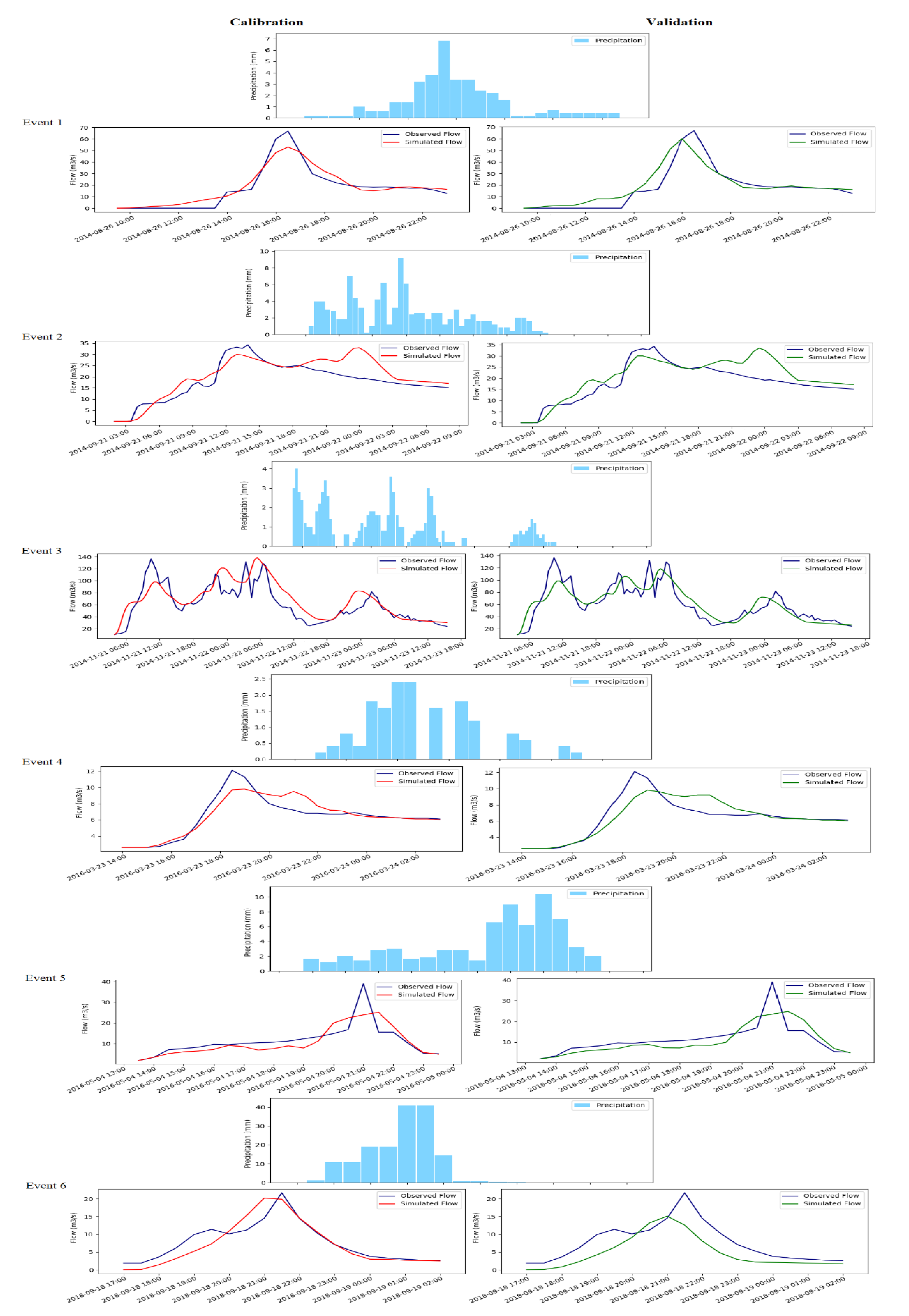
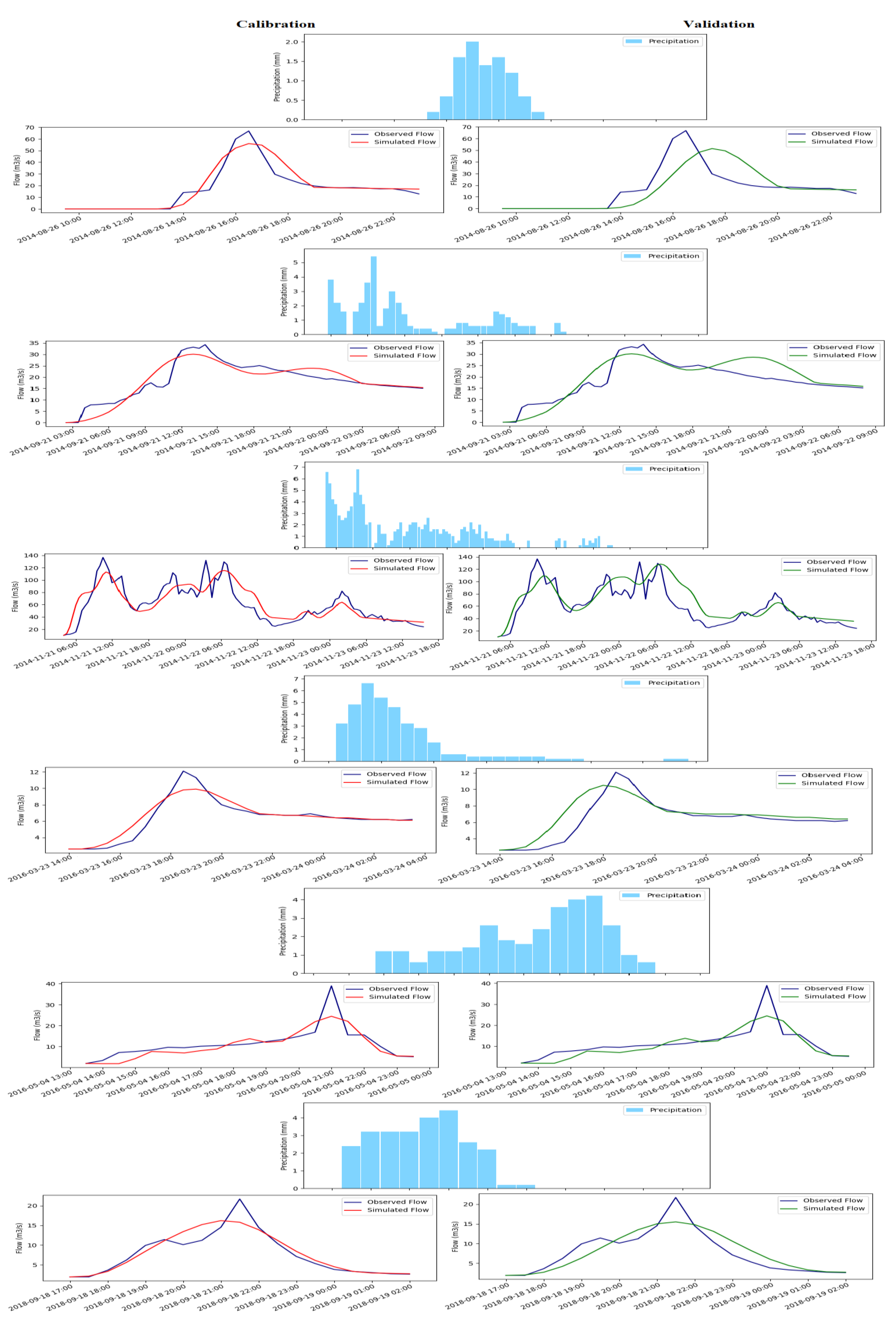
Figure 5 illustrates the observed and simulated hydrographs of calibration and validation for the six studied flood events from 2014 to 2018 using the IMERG Early precipitation product. The model reproduced the observed discharge curves and their trends fairly well throughout the calibration and validation.
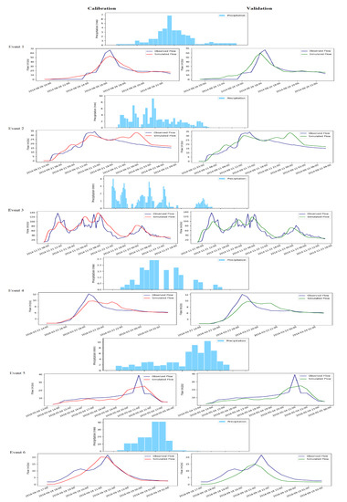
Figure 5.
Calibration and validation hydrographs, of IMERG Early precipitation product between 2014 and 2018.
The results showed that IMERG Early is efficient at capturing intensive precipitation time series in the high mountains, as its latency time is about 4 h. The rise and recession curves were overall well-reproduced for all events, and the peak flow rate was generally achieved for all events in the calibration and validation portions.
However, it is highlighted that IMERG Early was able to simulate accurately the streamflow at events 1 and 3 for the heavy flash flood category, and to slightly overestimate the simulated streamflow volumes at events 2, 4, 5, and 6 for both moderate and low flash flood categories.
Nevertheless, the results indicate a good fit among the data sets with an NSE between 0.60 and 0.91 in the calibration, and between 0.47 and 0.84 in the validation. The decrease in the validation criteria is because the IMERG Early product does not consider the initial humidity conditions due to its latency time.
4.4.2. Calibration and Validation of IMERG Late Events
The hydrographs in Figure 6 illustrate the comparative results of calibration and validation of the IMERG Late precipitation data.
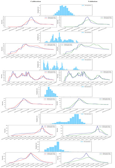
Figure 6.
Calibration and validation hydrographs, of IMERG-Late precipitation product between 2014 and 2018.
The model reproduced accurately the general flow pattern of the observed flow during the calibration and validation events. Furthermore, results showed that IMERG Late can estimate the intense precipitation time series better than its ancestor IMERG Early, due to its latency time of about 14 h, which allows it to make some data adjustments.
However, the simulated flows were in good fit with the observed one during calibration and validation, with NSEs between 0.59 and 0.90, and between 0.54 and 0.90 respectively, showing that in the validation part, the consideration of the initial soil moisture condition was more meaningful for IMERG Late and clearly improved its validation results.
A significant improvement of the simulated flow volumes was noticed at events 1 and 3 in the heavy flash flood category, with a slight underestimation of precipitation in the moderate flash flood category on events 2, 5, and 6, followed by a good improvement of the curve shape and the simulated flow volume of event 4 at low flash flood category, noticing its higher capacity to detect the peak discharge.
4.4.3. Calibration and Validation of IMERG Final Events
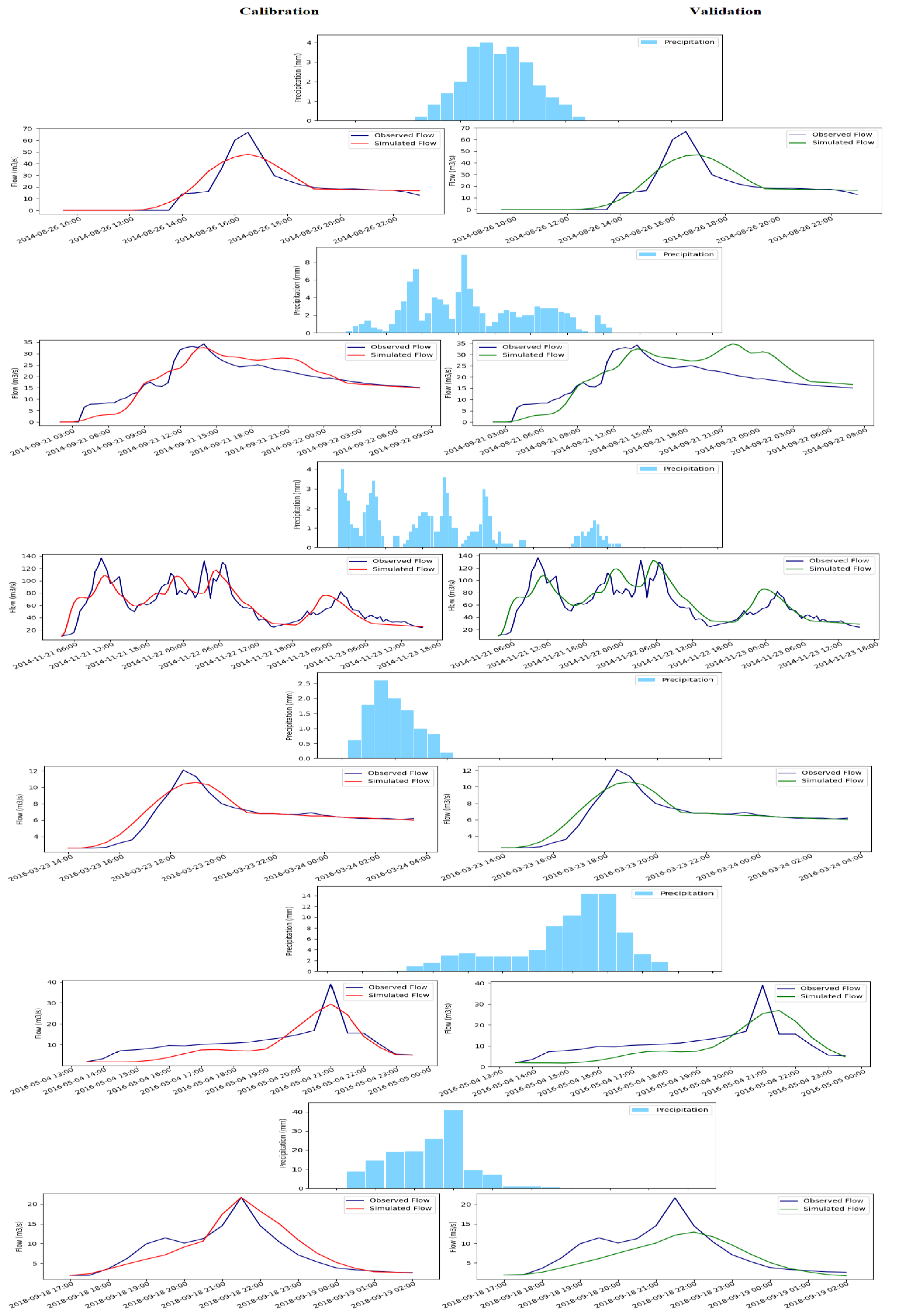
The results depicted in Figure 7 display that the simulated flows generated by the IMERG final run performed well for calibration and validation.
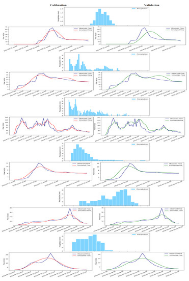
Figure 7.
Calibration and validation hydrographs, of IMERG-Finale precipitation product between 2014 and 2018.
The rise curves were generally well-reproduced, with peak flows mostly achieved for most events, while recession curves were mostly overestimated for the calibration and validation parts. However, it should be noticed that IMERG Final slightly overestimated the simulated event volumes for all flash flood categories.
Nevertheless, the results of the evaluation criteria indicate a good agreement between the datasets with NSEs between 0.68 and 0.90 in the calibration, and between 0.51 and 0.80 in the validation. Indeed, the decrease in the evaluation criteria in the validation results is because the IMERG Finale product is moderately adapted to flash flood simulations in mountainous regions compared to the IMERG Late product, but can give better results at lower altitudes.
However, this research is one of the first works that evaluate the GPM IMERG products in this region [12,15,16]. Hence, obtained results can be used to improve future IMERG strategies affiliated with arid mountainous zones, since poorly gauged basins in these regions urgently need accurate rainfall data for disaster management and flood forecasting.
5. Conclusions
This research assessed the effectiveness of the GPM IMERG V06 products components, in the semi-arid Zat basin, which is not a well-gauged mountainous watershed, equipped with only one downstream measuring station that these data were used as the benchmark, over the four-year period from 2014 to 2018. The assessment of the IMERG products was achieved by considering four approaches (1) Spatial distribution of precipitation and its influence on runoff at the outlet are identified, (2) Data pre-processing and bias correction using the CDF function and QM method. (3) Comparative statistical valuation of the 3 IMERG data, with a determination of their abilities to detect various precipitation types, (4) Calibration of the IMERG under the HEC-HMS model by comparing them to the gage data, and validation of the SPP products considering the initial soil conditions.
The principal findings of this research are:
- (1)
- The QM is an effective process for correcting the bias of satellite precipitation estimates when ground precipitation is not available. The statistical evaluation findings of the QM method indicated that IMERG_L showed a moderate improvement and performed slightly superior to IMERG_E and IMERG_F. Overall, the lack of rain-gauge stations prevents the correct evaluation of earth observation products and leads to an underestimation of the product’s performance, which is our case.
- (2)
- Regarding the effectiveness of the three SPPs, IMERG Late surpassed the remaining two SPPs in the majority of statistical metrics. However, IMERG Final ranked second to IMERG Early which slightly overestimated total precipitation.
- (3)
- The results of the hydrological model indicate that the IMERG Early, Late, and Final products achieved satisfactory hydrological performance with mean evaluation criteria (NSE) of 0.77, 0.82, and 0.82 respectively. However, during the validation of the flood events, by considering the initial soil conditions, IMERG_F and IMERG_E showed a significant overestimation of the discharge of 13%, and 10% respectively, while IMERG_L performed satisfactorily in the validation part with an avg. value of NSE = 0.69.
- (4)
- In synthesis, we can report that IMERG Early is quite reliable for capturing short-term extreme rainfall events of high intensity, and less suitable for precipitation events of medium and long duration and low intensity. Due to its 4-h latency, this product is not sensitive to the initial soil moisture conditions applied during the validation, which explains the decrease in these evaluation criteria, especially the NSE of 10%.
- (5)
- Furthermore, the IMERG Late precipitation product has the aptitude to estimate the precipitation time series at different flood intensities and durations, better than the IMERG Early and Final products. However, due to its time latency of about 14 h, it allows for some data adjustments, e.g., to take into account the initial soil moisture condition which clearly improved its validation results.
- (6)
- Nevertheless, the IMERG Finale product is not well adapted to short duration flash flood simulations in mountainous regions, which explains further the decrease in validation performance criteria by 13%. This may be due to the rugged topography of the region, which is characterized by mainly high-altitude areas.
Altogether, this research has the potential to provide earth observation precipitation users with reliable guidance for choosing between several IMERG precipitation products in the context of flood forecasting. A framework that comprehensively studies the characteristics of IMERG precipitation products in many aspects in the case of a mountainous, semi-arid and poorly gauged watershed.
Author Contributions
Conceptualization, M.B.; methodology, M.B. and A.A.; software, M.B.; validation, M.B.; formal analysis, M.B. and S.K.; resources, M.B. and S.K.; data curation, M.B.; writing—original draft preparation, M.B.; writing—review and editing, M.B., A.A., S.K., N.-E.L. and A.C.; supervision, A.A., N.-E.L. and S.K.; project administration, S.K. and N.-E.L.; funding acquisition, A.C. All authors have read and agreed to the published version of the manuscript.
Funding
The following work has been funded by the following projects: This work was funded by the projects: ERANETMED3-062/“CHAAMS Global Change: Assessment and Adaptation to Mediterranean Region Water Scarcity”, PRIMA-S2-ALTOS-2018/“Managing water resources within Mediterranean agrosystems by accounting for spatial structures and connectivities”, and APR&D multithématique 2020 CNRST-FOCP/GEANTech “Gestion durable de l’Eau en Agriculture: Innovation d’une approche synergique des Nouvelles Technologies et d’intelligence collective”.
Institutional Review Board Statement
Not applicable.
Data Availability Statement
Remote sensing data used in this study are freely accessible.
Conflicts of Interest
The authors declare no conflict of interest.
References
- Bollasina, M.A.; Ming, Y.; Ramaswamy, V. Anthropogenic Aerosols and the Weakening of the South Asian Summer Monsoon. Science 2011, 334, 502–505. [Google Scholar] [CrossRef] [PubMed]
- Pińskwar, I.; Choryński, A.; Graczyk, D.; Kundzewicz, Z.W. Observed Changes in Extreme Precipitation in Poland: 1991–2015 versus 1961–1990. Theor. Appl. Climatol. 2019, 135, 773–787. [Google Scholar] [CrossRef]
- Bonsal, B.; Peters, D.; Seglenieks, F.; Rivera, A.; Berg, A. Changes in Freshwater Availability across Canada. Canada’s Chang. Clim. Rep. 2019, pp. 261–342. Available online: https://natural-resources.canada.ca/sites/www.nrcan.gc.ca/files/energy/Climate-change/pdf/CCCR-Chapter6-ChangesInFreshwaterAvailabilityAcrossCanada.pdf (accessed on 2 February 2023).
- AghaKouchak, A.; Farahmand, A.; Melton, F.S.; Teixeira, J.; Anderson, M.C.; Wardlow, B.D.; Hain, C.R. Remote Sensing of Drought: Progress, Challenges and Opportunities. Rev. Geophys. 2015, 53, 452–480. [Google Scholar] [CrossRef]
- El Fels, A.E.A. Rainfall Regionalization and Variability of Extreme Precipitation Using Artificial Neural Networks: A Case Study from Western Central Morocco. J. Water Clim. Chang. 2021, 12, 1107. [Google Scholar] [CrossRef]
- Benkirane, M.; Laftouhi, N.E.; El Mansouri, B.; Salik, I.; Snineh, M.; El Ghazali, F.E.; Kamal, S.; Zamrane, Z. An Approach for Flood Assessment by Numerical Modeling of Extreme Hydrological Events in the Zat Watershed (High Atlas, Morocco). Urban Water J. 2020, 17, 381–389. [Google Scholar] [CrossRef]
- Kizza, M.; Rodhe, A.; Xu, C.-Y.; Ntale, H.K.; Halldin, S. Temporal Rainfall Variability in the Lake Victoria Basin in East Africa during the Twentieth Century. Theor. Appl. Climatol. 2009, 98, 119–135. [Google Scholar] [CrossRef]
- Dinku, T.; Funk, C.; Peterson, P.; Maidment, R.; Tadesse, T.; Gadain, H.; Ceccato, P. Validation of the CHIRPS Satellite Rainfall Estimates over Eastern Africa. Q. J. R. Meteorol. Soc. 2018, 144, 292–312. [Google Scholar] [CrossRef]
- Ageet, S.; Fink, A.H.; Maranan, M.; Diem, J.E.; Hartter, J.; Ssali, A.L.; Ayabagabo, P. Validation of Satellite Rainfall Estimates over Equatorial East Africa. J. Hydrometeorol. 2022, 23, 129–151. [Google Scholar] [CrossRef]
- Monsieurs, E.; Kirschbaum, D.B.; Tan, J.; Maki Mateso, J.-C.; Jacobs, L.; Plisnier, P.-D.; Thiery, W.; Umutoni, A.; Musoni, D.; Bibentyo, T.M.; et al. Evaluating TMPA Rainfall over the Sparsely Gauged East African Rift. J. Hydrometeorol. 2018, 19, 1507–1528. [Google Scholar] [CrossRef]
- Ouaba, M.; El Khalki, E.M.; Saidi, M.E.; Alam, M.J. Bin Estimation of Flood Discharge in Ungauged Basin Using GPM-IMERG Satellite-Based Precipitation Dataset in a Moroccan Arid Zone. Earth Syst. Environ. 2022, 6, 541–556. [Google Scholar] [CrossRef]
- Panegrossi, G.; Casella, D.; Dietrich, S.; Marra, A.C.; Sano, P.; Mugnai, A.; Baldini, L.; Roberto, N.; Adirosi, E.; Cremonini, R.; et al. Use of the GPM Constellation for Monitoring Heavy Precipitation Events Over the Mediterranean Region. IEEE J. Sel. Top. Appl. Earth Obs. Remote Sens. 2016, 9, 2733–2753. [Google Scholar] [CrossRef]
- Panegrossi, G.; Marra, A.C.; Sanò, P.; Baldini, L.; Casella, D.; Porcù, F. Heavy Precipitation Systems in the Mediterranean Area: The Role of GPM. In Satellite Precipitation Measurement; Springer: Cham, Switzerland, 2020; pp. 819–841. [Google Scholar]
- Benkirane, M.; Laftouhi, N.-E.; Khabba, S.; Hera-Portillo, Á. de la Hydro Statistical Assessment of TRMM and GPM Precipitation Products against Ground Precipitation over a Mediterranean Mountainous Watershed (in the Moroccan High Atlas). Appl. Sci. 2022, 12, 8309. [Google Scholar] [CrossRef]
- Saouabe, T.; Naceur, K.A.; El Khalki, E.M.; Hadri, A.; Saidi, M.E. GPM-IMERG Product: A New Way to Assess the Climate Change Impact on Water Resources in a Moroccan Semi-Arid Basin. J. Water Clim. Chang. 2022, 13, 2559–2576. [Google Scholar] [CrossRef]
- Li, Z.; Yang, D.; Hong, Y. Multi-Scale Evaluation of High-Resolution Multi-Sensor Blended Global Precipitation Products over the Yangtze River. J. Hydrol. 2013, 500, 157–169. [Google Scholar] [CrossRef]
- Massari, C.; Brocca, L.; Pellarin, T.; Abramowitz, G.; Filippucci, P.; Ciabatta, L.; Maggioni, V.; Kerr, Y.; Fernandez Prieto, D. A Daily/25 Km Short-Latency Rainfall Product for Data Scarce Regions Based on the Integration of the GPM IMERG Early Run with Multiple Satellite Soil Moisture Products. Hydrol. Earth Syst. Sci. Discuss. 2020, 24, 2687–2710. [Google Scholar] [CrossRef]
- Einfalt, T.; Arnbjerg-nielsen, K.; Golz, C.; Jensen, N.; Quirmbach, M.; Vaes, G.; Vieux, B. Towards a Roadmap for Use of Radar Rainfall Data in Urban Drainage. J. Hydrol. 2004, 299, 186–202. [Google Scholar] [CrossRef]
- Xu, R.; Tian, F.; Yang, L.; Hu, H.; Lu, H.; Hou, A. Ground Validation of GPM IMERG and Trmm 3B42V7 Rainfall Products over Southern Tibetan Plateau Based on a High-Density Rain Gauge Network. J. Geophys. Res. 2017, 122, 910–924. [Google Scholar] [CrossRef]
- Tang, G.; Zeng, Z.; Long, D.; Guo, X.; Yong, B.; Zhang, W.; Hong, Y. Statistical and Hydrological Comparisons between TRMM and GPM Level-3 Products over a Midlatitude Basin: Is Day-1 IMERG a Good Successor for TMPA 3B42V7? J. Hydrometeorol. 2016, 17, 121–137. [Google Scholar] [CrossRef]
- Hou, A.Y.; Kakar, R.K.; Neeck, S.; Azarbarzin, A.A.; Kummerow, C.D.; Kojima, M.; Oki, R.; Nakamura, K.; Iguchi, T. The Global Precipitation Measurement Mission. Bull. Am. Meteorol. Soc. 2014, 95, 701–722. [Google Scholar] [CrossRef]
- Yi, L.; Zhang, W.; Wang, K. Evaluation of Heavy Precipitation Simulated by the WRF Model Using 4D-Var Data Assimilation with TRMM 3B42 and GPM IMERG over the Huaihe River Basin, China. Remote Sens. 2018, 10, 646. [Google Scholar] [CrossRef]
- Scheel, M.L.M.; Rohrer, M.; Huggel, C.; Santos Villar, D.; Silvestre, E.; Huffman, G.J. Evaluation of TRMM Multi-Satellite Precipitation Analysis (TMPA) Performance in the Central Andes Region and Its Dependency on Spatial and Temporal Resolution. Hydrol. Earth Syst. Sci. 2011, 15, 2649–2663. [Google Scholar] [CrossRef]
- Tapiador, F.J.; Navarro, A.; García-Ortega, E.; Merino, A.; Sánchez, J.L.; Marcos, C.; Kummerow, C. The Contribution of Rain Gauges in the Calibration of the IMERG Product: Results from the First Validation over Spain. J. Hydrometeorol. 2020, 21, 161–182. [Google Scholar] [CrossRef]
- Yong, B.; Liu, D.; Gourley, J.J.; Tian, Y.; Huffman, G.J.; Ren, L.; Hong, Y. Global View of Real-Time TRMM Multisatellite Precipitation Analysis: Implications for Its Successor Global Precipitation Measurement Mission. Bull. Am. Meteorol. Soc. 2015, 96, 283–296. [Google Scholar] [CrossRef]
- Gebregiorgis, A.S.; Kirstetter, P.; Hong, Y.E.; Gourley, J.J.; Huffman, G.J.; Petersen, W.A.; Xue, X.; Schwaller, M.R. To What Extent Is the Day 1 GPM IMERG Satellite Precipitation Estimate Improved as Compared to TRMM TMPA-RT? J. Geophys. Res. Atmos. 2018, 123, 1694–1707. [Google Scholar] [CrossRef]
- Ammar, H. Elsheikh Applications of Machine Learning in Friction Stir Welding: Prediction of Joint Properties, Real-Time Control and Tool Failure Diagnosis. Eng. Appl. Artif. Intell. 2023, 121, 105961. [Google Scholar] [CrossRef]
- Gaona, M.F.R.; Overeem, A.; Leijnse, H.; Uijlenhoet, R. First-Year Evaluation of GPM Rainfall over the Netherlands: IMERG Day 1 Final Run (V03D). J. Hydrometeorol. 2016, 17, 2799–2814. [Google Scholar] [CrossRef]
- Gao, Y.; Wu, T.; Wang, J.; Tang, S. Evaluation of GPM Dual-Frequency Precipitation Radar (DPR) Rainfall Products Using the Rain Gauge Network over China. J. Hydrometeorol. 2021, 22, 547–559. [Google Scholar] [CrossRef]
- Liu, Z. Comparison of Integrated Multisatellite Retrievals for GPM (IMERG) and TRMM Multisatellite Precipitation Analysis (TMPA) Monthly Precipitation Products: Initial Results. J. Hydrometeorol. 2016, 17, 777–790. [Google Scholar] [CrossRef]
- Prakash, S.; Mitra, A.K.; AghaKouchak, A.; Liu, Z.; Norouzi, H.; Pai, D.S. A Preliminary Assessment of GPM-Based Multi-Satellite Precipitation Estimates over a Monsoon Dominated Region. J. Hydrol. 2018, 556, 865–876. [Google Scholar] [CrossRef]
- Sharifi, E.; Steinacker, R.; Saghafian, B. Assessment of GPM-IMERG and Other Precipitation Products against Gauge Data under Different Topographic and Climatic Conditions in Iran: Preliminary Results. Remote Sens. 2016, 8, 135. [Google Scholar] [CrossRef]
- Tang, G.; Ma, Y.; Long, D.; Zhong, L.; Hong, Y. Evaluation of GPM Day-1 IMERG and TMPA Version-7 Legacy Products over Mainland China at Multiple Spatiotemporal Scales. J. Hydrol. 2016, 533, 152–167. [Google Scholar] [CrossRef]
- Wu, Y.; Zhang, Z.; Huang, Y.; Jin, Q.; Chen, X.; Chang, J. Evaluation of the GPM IMERG v5 and TRMM 3B42 v7 Precipitation Products in the Yangtze River Basin, China. Water 2019, 11, 1459. [Google Scholar] [CrossRef]
- AghaKouchak, A.; Mehran, A.; Norouzi, H.; Behrangi, A. Systematic and Random Error Components in Satellite Precipitation Data Sets. Geophys. Res. Lett. 2012, 39, e1–e7. [Google Scholar] [CrossRef]
- Kimani, M.; Hoedjes, J.; Su, Z. An Assessment of Satellite-Derived Rainfall Products Relative to Ground Observations over East Africa. Remote Sens. 2017, 9, 430. [Google Scholar] [CrossRef]
- Tang, L.; Tian, Y.; Yan, F.; Habib, E. An Improved Procedure for the Validation of Satellite-Based Precipitation Estimates. Atmos. Res. 2015, 163, 61–73. [Google Scholar] [CrossRef]
- Sadeghi, M.; Asanjan, A.A.; Faridzad, M.; Nguyen, P.; Hsu, K.; Sorooshian, S.; Braithwaite, D. PERSIANN-CNN: Precipitation Estimation from Remotely Sensed Information Using Artificial Neural Networks–Convolutional Neural Networks. J. Hydrometeorol. 2019, 20, 2273–2289. [Google Scholar] [CrossRef]
- Alsaiari, A.O.; Moustafa, E.B.; Alhumade, H.; Abulkhair, H.; Elsheikh, A. A Coupled Artificial Neural Network with Artificial Rabbits Optimizer for Predicting Water Productivity of Different Designs of Solar Stills. Adv. Eng. Softw 2023, 175, 103315. [Google Scholar] [CrossRef]
- Fang, G.H.; Yang, J.; Chen, Y.N.; Zammit, C. Comparing Bias Correction Methods in Downscaling Meteorological Variables for a Hydrologic Impact Study in an Arid Area in China. Hydrol. Earth Syst. Sci. 2015, 19, 2547–2559. [Google Scholar] [CrossRef]
- Serrat-Capdevila, A.; Merino, M.; Valdes, J.; Durcik, M. Evaluation of the Performance of Three Satellite Precipitation Products over Africa. Remote Sens. 2016, 8, 836. [Google Scholar] [CrossRef]
- Huffman, G.J.; Adler, R.F.; Bolvin, D.T.; Gu, G.; Nelkin, E.J.; Bowman, K.P.; Hong, Y.; Stocker, E.F.; Wolff, D.B. The TRMM Multisatellite Precipitation Analysis (TMPA): Quasi-Global, Multiyear, Combined-Sensor Precipitation Estimates at Fine Scales. J. Hydrometeorol. 2007, 8, 38–55. [Google Scholar] [CrossRef]
- Xie, P.; Xiong, A.-Y. A Conceptual Model for Constructing High-Resolution Gauge-Satellite Merged Precipitation Analyses. J. Geophys. Res. Atmos. 2011, 116, 47–64. [Google Scholar] [CrossRef]
- Katiraie-Boroujerdy, P.; Akbari Asanjan, A.; Chavoshian, A.; Hsu, K.; Sorooshian, S. Assessment of Seven CMIP5 Model Precipitation Extremes over Iran Based on a Satellite-based Climate Data Set. Int. J. Climatol. 2019, 39, 3505–3522. [Google Scholar] [CrossRef]
- Piani, C.; Haerter, J.O.; Coppola, E. Statistical Bias Correction for Daily Precipitation in Regional Climate Models over Europe. Theor. Appl. Climatol. 2010, 99, 187–192. [Google Scholar] [CrossRef]
- Le Coz, C.; van de Giesen, N. Comparison of Rainfall Products over Sub-Saharan Africa. J. Hydrometeorol. 2020, 21, 553–596. [Google Scholar] [CrossRef]
- Boudhar, A.; Hanich, L.; Boulet, G.; Duchemin, B.; Berjamy, B.; Chehbouni, A. Evaluation of the Snowmelt Runoff Model in the Moroccan High Atlas Mountains Using Two Snow-Cover Estimates. Hydrol. Sci. J. 2009, 54, 1094–1113. [Google Scholar] [CrossRef]
- Hanich, L.; Chehbouni, A.; Gascoin, S.; Boudhar, A.; Jarlan, L.; Tramblay, Y.; Boulet, G.; Marchane, A.; Baba, M.W.; Kinnard, C.; et al. Snow Hydrology in the Moroccan Atlas Mountains. J. Hydrol. Reg. Stud. 2022, 42, 101101. [Google Scholar] [CrossRef]
- Baba, M.W.; Gascoin, S.; Kinnard, C.; Marchane, A.; Hanich, L. Effect of Digital Elevation Model Resolution on the Simulation of the Snow Cover Evolution in the High Atlas. Water Resour. Res. 2019, 55, 5360–5378. [Google Scholar] [CrossRef]
- El Arabi, E.H.; Diez, J.B.; Broutin, J.; Essamoud, R. Première Caractérisation Palynologique Du Trias Moyen Dans Le Haut Atlas; Implications Pour l’initiation Du Rifting Téthysien Au Maroc. Comptes Rendus Geosci. 2006, 338, 641–649. [Google Scholar] [CrossRef]
- Chaponnière, A.; Boulet, G.; Chehbouni, A.; Aresmouk, M. Understanding Hydrological Processes with Scarce Data in a Mountain Environment. Hydrol. Process. 2008, 22, 1908–1921. [Google Scholar] [CrossRef]
- Rudolf, B.; Beck, C.; Grieser, J.; Schneider, U. Global Precipitation climatology center of the GPCC. Glob. Precip. Climatol. Cent. Rep. 2005, 1–8. [Google Scholar]
- Huffman, G.J.; Bolvin, D.T.; Braithwaite, D.; Hsu, K.; Joyce, R.; Kidd, C.; Nelkin, E.J.; Sorooshian, S.; Tan, J. Algorithm Theoretical Basis Document (ATBD) Version 06. NASA Global Precipitation Measurement (GPM) Integrated Multi-satellitE Retrievals for GPM (IMERG). 2019. Available online: Https://Gpm.Nasa.Gov/Sites/Default/Files/Document_files/IMERG_ATBD_V06_0.Pdf (accessed on 2 February 2023).
- U.S. Army Corps of Engineers Hydrologic Modeling System. In Application Guide; U.S. Army Corps of Engineers: Davis, CA, USA, 2017; p. 158.
- Lashkari, A.; Salehnia, N.; Asadi, S.; Paymard, P.; Zare, H.; Bannayan, M. Evaluation of Different Gridded Rainfall Datasets for Rainfed Wheat Yield Prediction in an Arid Environment. Int. J. Biometeorol. 2018, 62, 1543–1556. [Google Scholar] [CrossRef] [PubMed]
- Condom, T.; Rau, P.; Espinoza, J.C. Correction of TRMM 3B43 Monthly Precipitation Data over the Mountainous Areas of Peru during the Period 1998-2007. Hydrol. Process. 2011, 25, 1924–1933. [Google Scholar] [CrossRef]
- Katiraie-Boroujerdy, P.-S.; Rahnamay Naeini, M.; Akbari Asanjan, A.; Chavoshian, A.; Hsu, K.; Sorooshian, S. Bias Correction of Satellite-Based Precipitation Estimations Using Quantile Mapping Approach in Different Climate Regions of Iran. Remote Sens. 2020, 12, 2102. [Google Scholar] [CrossRef]
- Brocca, L.; Hasenauer, S.; Lacava, T.; Melone, F.; Moramarco, T.; Wagner, W.; Dorigo, W.; Matgen, P.; Martínez-Fernández, J.; Llorens, P.; et al. Soil Moisture Estimation through ASCAT and AMSR-E Sensors: An Intercomparison and Validation Study across Europe. Remote Sens. Environ. 2011, 115, 3390–3408. [Google Scholar] [CrossRef]
- Fang, L.; Hain, C.R.; Zhan, X.; Anderson, M.C. An Inter-Comparison of Soil Moisture Data Products from Satellite Remote Sensing and a Land Surface Model. Int. J. Appl. Earth Obs. Geoinf. 2016, 48, 37–50. [Google Scholar] [CrossRef]
- Reichle, R.H. Bias Reduction in Short Records of Satellite Soil Moisture. Geophys. Res. Lett. 2004, 31, L19501. [Google Scholar] [CrossRef]
- Daniel, S.W. Wilks Statistical Methods in the Atmospheric Sciences. Academic Press: Cambridge, MA, USA, 2011; ISBN 0123850223. [Google Scholar]
- Themeßl, M.J.; Gobiet, A.; Heinrich, G. Empirical-Statistical Downscaling and Error Correction of Regional Climate Models and Its Impact on the Climate Change Signal. Clim. Chang. 2012, 112, 449–468. [Google Scholar] [CrossRef]
- USACE Hydrologic Modeling System (HEC-HMS) User’s Manual: Version 4.3.0; Hydrologic Engineering Center: Davis, CA, USA, 2018.
- Arlen, D. Feldman Hydrologic Modeling System HEC-HMS: Technical Reference Manual; US Army Corps of Engineers, Hydrologic Engineering Center: Davis, CA, USA.
- El Khalki, E.M.; Tramblay, Y.; El Mehdi Saidi, M.; Bouvier, C.; Hanich, L.; Benrhanem, M.; Alaouri, M. Comparison of Modeling Approaches for Flood Forecasting in the High Atlas Mountains of Morocco. Arab. J. Geosci. 2018, 11, 410. [Google Scholar] [CrossRef]
- Moriasi, D.N.; Arnold, J.G.; Van Liew, M.W.; Bingner, R.L.; Harmel, R.D.; Veith, T.L. Veith Model Evaluation Guidelines for Systematic Quantification of Accuracy in Watershed Simulations. Trans. ASABE 2007, 50, 885–900. [Google Scholar] [CrossRef]
- Valdés-Pineda, R.; Demaría, E.M.C.; Valdés, J.B.; Wi, S.; Serrat-Capdevilla, A. Bias Correction of Daily Satellite-Based Rainfall Estimates for Hydrologic Forecasting in the Upper Zambezi, Africa. Hydrol. Earth Syst. Sci. Discuss. 2016, 1–28. [Google Scholar] [CrossRef]
- Ramesh, V. Application of the HEC-HMS Model for Runoff Simulation in the Krishna Basin. Master’s Thesis, National Institute of Technology Karnataka, Surathkal, India, 2017. [Google Scholar] [CrossRef]
- Tramblay, Y.; Bouaicha, R.; Brocca, L.; Dorigo, W.; Bouvier, C.; Camici, S.; Servat, E. Estimation of Antecedent Wetness Conditions for Flood Modelling in Northern Morocco. Hydrol. Earth Syst. Sci. 2012, 16, 4375–4386. [Google Scholar] [CrossRef]
- Chen, S.; Hong, Y.; Gourley, J.J.; Huffman, G.J.; Tian, Y.; Cao, Q.; Yong, B.; Kirstetter, P.E.; Hu, J.; Hardy, J.; et al. Evaluation of the Successive V6 and V7 TRMM Multisatellite Precipitation Analysis over the Continental United States. Water Resour. Res. 2013, 49, 8174–8186. [Google Scholar] [CrossRef]
Disclaimer/Publisher’s Note: The statements, opinions and data contained in all publications are solely those of the individual author(s) and contributor(s) and not of MDPI and/or the editor(s). MDPI and/or the editor(s) disclaim responsibility for any injury to people or property resulting from any ideas, methods, instructions or products referred to in the content. |
© 2023 by the authors. Licensee MDPI, Basel, Switzerland. This article is an open access article distributed under the terms and conditions of the Creative Commons Attribution (CC BY) license (https://creativecommons.org/licenses/by/4.0/).


