Abstract
By addressing the imbalanced proportions of the data category samples in the velocity structure function of the LiDAR turbulence identification model, we propose a flight turbulence identification model utilizing both a conditional generative adversarial network (CGAN) and extreme gradient boosting (XGBoost). This model can fully learn small- and medium-sized turbulence samples, reduce the false alarm rate, improve robustness, and maintain model stability. Model training involves constructing a balanced dataset by generating samples that conform to the original data distribution via the CGAN. Subsequently, the XGBoost model is iteratively trained on the sample set to obtain the flight turbulence classification level. Experiments show that the turbulence recognition accuracy achieved on the CGAN-generated augmented sample set improves by 15%. Additionally, when incorporating LiDAR-obtained wind field data, the performance of the XGBoost model surpasses that of traditional classification algorithms such as K-nearest neighbours, support vector machines, and random forests by 14%, 8%, and 5%, respectively, affirming the excellence of the model for turbulence classification. Moreover, a comparative analysis conducted on a Zhongchuan Airport flight crew report showed that the model achieved a 78% turbulence identification accuracy, indicating enhanced recognition ability under data-imbalanced conditions. In conclusion, our CGAN/XGBoost model effectively addresses the proportion imbalance issue.
1. Introduction
Turbulence is a phenomenon resulting from disorderly temperature changes within the atmosphere, leading to density variations and fluctuations in the refractive index. These fluctuations feature temporal discontinuities and spatial heterogeneity [1] and pose significant hazards to aviation by inducing turbulence during flight. Severe turbulence can result in sudden changes to an aircraft’s altitude, leading to loss of control by the pilot [2]. Doppler light detection and ranging (LiDAR) is a widely used remote sensing method for measuring atmospheric parameters in the lower troposphere. It is capable of measuring wind profiles ranging from tens to hundreds of metres and even up to one kilometre at low altitudes. It can also measure turbulence parameter profiles, such as the constant of the refractive index mechanism [3]. The principle of the optical Doppler frequency shift between reference radiation and backscattered radiation is utilized by Doppler LiDAR to measure the radial velocity [4]. The effective eddy current dissipation rate (EDR) is commonly used to represent turbulence information and provide pilots with standard International Civil Aviation organization (ICAO) turbulence reports [5].
In recent years, numerous airports have implemented models and hardware for detecting wind shear [6]. To address the nonuniformity and nonstationary nature of the collected layer data, Boilley A et al. [7] conducted research and experiments utilizing remote sensing technology, specifically Doppler LiDAR in conjunction with a stable boundary layer (SBL), to measure the average wind speed and velocity change contours. Ahijevych D et al. [8] employed data mining and statistical learning methods, i.e., random forests (RFs), to generate mesoscale convective systems and investigate their 2 h predictive capabilities. Pichugina YL et al. [9] significantly reduced the prediction error and false alarm rate of the EDR by implementing a gradient-enhanced regression tree method to predict turbulence information and training and evaluating the residual dissipation rate. Jincheng Zhang et al. [10] developed a deep neural network utilizing the Navier-Stokes equation as a means of accurately describing atmospheric flow. This model requires only sparse LiDAR measurement data for learning, following which it can predict the entire domain (which is unmeasurable). Shinya Mizuno et al. [11] utilized principal component analysis in combination with the K-means method to generate risk clusters with heightened turbulence occurrence probabilities; they, subsequently, used the risk clustering data as monitoring data while employing support vector machines (SVMs) for turbulence occurrence prediction.
Karthik Duraisamy et al. [12] employed statistical inference to characterize model coefficients and estimate differences and utilized machine learning to enhance turbulence models to gauge and mitigate model uncertainty. Subramaniam et al. [13] developed an improved method for generating confrontation networks, incorporated physical data to enrich low-resolution turbulence data, and validated the model’s increased generalization ability on a test set. Wang, C et al. [14] applied the extreme gradient boosting (XGBoost) algorithm to the conventional turbulence index dataset generated by a numerical weather forecast model for turbulence prediction and verified their results using unit reports, where the algorithm was found to perform well in terms of predicting the massive generated turbulence index data. Purohit et al. [15] utilized three machine learning algorithms, namely, SVMs, artificial neural networks, and XGBoost, to predict turbulence intensities based on numerical simulation datasets, where the XGBoost algorithm was found to provide the most accurate predictions. Jiang Liu et al. [16] used a conditional generative adversarial network (CGAN) to address the issue of imbalanced fault sample datasets, combining this network with the XGBoost-limited gradient scheme to train a fault prediction model, which was, subsequently, verified using actual field datasets. Jun Feng Jia et al. [17] explored optimization methods for compressive strength prediction utilizing multiple integrated machine learning methods. Finally, the application of a conditional countermeasure CGAN was found to resolve problems related to data scarcity or a lack of specific levels.
This article employs a CGAN and XGBoost to mitigate data instability and losses. This study utilizes wind measurement data obtained from a LiDAR experimental platform during the period of 2018–2019 as a basis for calculating different values of the structure function; this approach corresponds to proportional expansion based on the interval distance using the velocity structure function method in the turbulence model. Subsequently, a dataset is constructed. As the proportions of turbulence class samples in the original dataset are not balanced, this paper presents a flight turbulence identification model named CGAN-XGBoost. The model employs a CGAN to create designated labelled samples with different turbulence levels, expands the rare turbulence class samples, and increases the diversity of the dataset. According to the classification performance results, the XGBoost model achieves improvements of 14%, 8%, and 5% over the traditional K-nearest neighbours’ algorithm, a support vector machine, and a random forest, respectively. Based on a comparison and an analysis conducted on a crew report from Nakagawa Airport, the proposed model has a recognition accuracy of 78% for turbulence, effectively achieving an improved ability to recognize turbulence under imbalance data conditions.
2. Materials and Methods
2.1. Data Collection
When training the CGAN model, an augmented sample set was used for data expansion to avoid data singularity and instability. This article employed the 1.55μm Doppler wind LiDAR system located at Lanzhou Zhongchuan Airport to obtain experimental measurements. To improve its adaptation to the dissipation characteristics of turbulence, as depicted in Figure 1, the Doppler LiDAR system utilized the PPI scanning method [18].
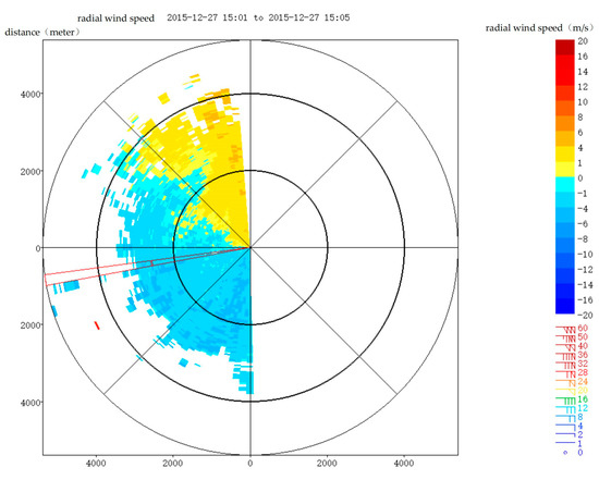
Figure 1.
LiDAR PPI scanning approach.
Wind speed data obtained from the aforementioned radar system from 2018 to 2019 were selected for research purposes. Table 1 displays the parameters of the experimental LiDAR platform. The acquired wind speed data were initially partitioned into sectors and preprocessed. Subsequently, the VSF method was implemented to calculate the corresponding velocity structure function values during the proportional expansion process based on the interval distance, thus constructing a dataset for training purposes.

Table 1.
Relevant LiDAR parameters.
2.2. Methods
2.2.1. Sector Division
The sector size for turbulence with different scales in the scanning area could be freely adjusted [19]. The specific division process involved dividing the entire scanning area into several sectors, each of which comprised radial lines and distance gates. To prevent a wind field sampling rate that was too low during the scanning process, overlapping scanning was employed [20]. The radial lines were moved by in the direction of increasing azimuth angle, and the moving radial lines and those within the adjacent sector formed a new scanning sector. Overlapping scanning was also employed in the radial direction. Last, each subsector and its adjacent subsectors overlapped by a distance gate containing radial lines in the azimuth and radial directions. The values of and were adjusted based on turbulence at different scales, which corresponded to sectors of varying sizes.
The scanning sector partitioning diagram is shown in Figure 2. Based on the characteristics of the Doppler LiDAR data measured at Lanzhou Airport and the range of the flight turbulence scales, this paper defined the azimuth interval between adjacent radial lines as 5°, the radar’s starting wind speed measurement point as 45 m, and the distance between distance gates as 30 m. In the horizontal azimuth, each 30° and 300 m of radial distance were divided into a sector.

Figure 2.
Schematic diagram of scanning sector division.
2.2.2. Conditional Generation of Countermeasure Networks
The concept of generative adversarial networks (GANs) entailed “playing games” between generators and discriminators, continuously optimizing the generated results [21]. The generator’s primary task was to generate samples that approximate real data under the influence of random noise, while the function of the discriminator was to differentiate between the generated and real samples. The objective function of the original GAN was defined as follows:
where represents the expected value of the distribution function, represents the training sample, represents random noise, represents the training sample distribution, represents the distribution of the random noise, represents the sample generated by the random noise, represents the probability of judging whether the sample is true, and represents the probability of judging whether the sample is true.
The original GAN fails to control the sample generation process, making it challenging to achieve training model stability. To remedy this issue, Liu XB and colleagues [22] proposed conditional GANs (CGANs). A CGAN incorporates the idea of supervised learning into the generator, transforming the probability assessment of the original CGAN into a conditional probability, generating corresponding outputs based on the joint action of the input category tags and random noise. In the CGAN model, data are classified and combined with random noise to generate more datasets. Generators and discriminators are continuously trained to distinguish between the generated samples and real samples. Figure 3 shows the model structure of the CGAN. The objective function of the CGAN is defined as follows:
where is the sample generated under conditions based on random noise , and is the probability that the sample output by the discriminator is the sample corresponding to the conditions.

Figure 3.
Model structure of a CGAN.
2.2.3. Loss Function
The XGBoost algorithm is an enhanced version of the gradient lifting algorithm that combines multiple weak learners to construct an integrated model with strong learning abilities to perform learning tasks and produce high-performance results. The objective function of the XGBoost algorithm comprises a loss function that measures the training errors and the complexity of the tree model.
The objective function of the XGBoost model is
where is the first derivative of the loss function, and is the second derivative of the loss function.
is the loss function; is the predicted value of the sample; is the true value of the sample; and is a regular item.
The regularized expression in the objective function is
where is the number of leaf nodes in the tree, representing the last predicted category for each branch; is the weight of the leaf nodes in the tree; and the complexity parameters and control the weights of the leaf nodes.
In XGBoost, the second-order Taylor expansion of the objective function is performed. Assuming that the loss function uses the mean squared error, the objective function can be written as
Then, by differentiating the above equation and setting the derivative equal to 0, the optimal weight of the leaf node can be obtained as :
2.2.4. Velocity Structure Function
During the LiDAR detection process, problematic factors arose, such as the radar’s cumulative error, leading to significant dimensional differences between certain points and their adjacent measurement points. Data magnitude differences could result in the feature data with larger magnitudes in the dataset having more extensive impacts on the overall recognition and classification process, which could slow down the iterative procedure of the recognition model. Additionally, considering that CGANs can efficiently learn data between 0 and 1, data normalization was used to eliminate the dimensional effects between the data. The original data underwent a linear transformation that mapped them to the [0, 1] interval, ensuring that the feature data were on the same order of magnitude. The formula for data normalization was as follows:
where xmax and xmin are the maximum and minimum data values, respectively.
Due to the spatial structure of turbulence, determining the intensity of the turbulence fluctuation in a sector required calculating the velocity structure function’s values for various lag distances that were proportionately expanded based on the interval distance [23]. In atmospheric turbulence, the air flow velocity comprised the average wind speed and fluctuating wind speed. First, the spatial averaging method calculated the average wind speed. Second, the fluctuating velocity of the turbulence was calculated based on the difference between the radial wind speed and the average wind speed as measured by the LiDAR system.
The structure function essentially calculated the pulsation velocity differences between different lag distances in each subsector that are proportionally expanded based on the interval distance [24]; this was expressed as a statistical description of the pulsation velocity difference:
In the formula, , refers to the total number of velocity fluctuations, and is an unbiased estimate of the radar measurement error.
Based on Kolmogorov’s isotropic turbulence theory and relevant experiments, when the current structure function’s interval distance (s) was significantly smaller than the scale of isotropic turbulence, the turbulence’s structure function could be expressed as follows:
where is the Kolmogorov constant, and is the dissipation rate of the turbulence.
By combining the velocity structure function in Formula (8) with Formula (9), the corresponding EDR could be obtained. In this paper, the velocity structure function was used as the dataset, and the EDR was used as the dataset label to train the flight turbulence identification model.
The dataset utilized in this model included data on the velocity structure function collected between 2018 and 2019, totalling 29,300 items. The features included 11 tag items, with the EDR tag being the 11th item in the dataset. Partial velocity structure function dataset styles are presented in Table 2.
Table 2.
Partial dataset for the velocity structure function.
Table 3 illustrates that ICAO- and relevant scholar-assessed turbulence intensity and harmfulness values based on the numerical EDR values and categorizes turbulence into three levels: mild turbulence, moderate turbulence, and severe turbulence.
Table 3.
Turbulence intensity levels.
Figure 4 presents the distribution of the labelled samples, revealing that turbulence below the mild level represents 72% of the data, moderate turbulence represents 19% of the data, and severe turbulence represents 9% of the data. The number of severe turbulence samples is significantly less than the number of mild turbulence samples, resulting in imbalanced sample proportions for the categories in the data. When rare turbulence class data from the dataset are directly input into the recognition classification model for training, the classifier fails to learn adequately, negatively affecting its generalization ability and its classification accuracy for most class samples. To alleviate the impact of category imbalance on the accuracy of the recognition and classification model, the CGAN is utilized to generate a diversified labelled augmented sample set for the existing velocity structure function dataset, thereby enhancing the accuracy of subsequent flight turbulence recognition models.

Figure 4.
Distribution map of the labelled samples.
2.2.5. Model Structure
Figure 5 displays the framework of the flight turbulence identification model based on the CGAN and XGBoost. First, the wind speed data collected by the LiDAR system were processed via the VSF method to calculate the original dataset of velocity structure function values corresponding to different distances. Seventy percent of the dataset was utilized as the training sample set, and the remaining 30% was used as the test sample set. Second, the CGAN was trained on the training sample set to generate a labelled augmented sample set. Third, the XGBoost classifier was trained using the augmented sample set, and a turbulence recognition and classification model was developed. Finally, the test sample set was input into the trained flight turbulence identification model to test its effectiveness.
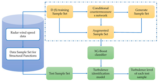
Figure 5.
Framework diagram of the CGAN-XGBoost-based flying turbulence recognition model.
2.3. Evaluation Metrics
This article used indicators such as precision (P), recall (R), F1 score (a comprehensive evaluation index), and accuracy (A) to evaluate the classification effect of the model. The calculation formulas were as follows:
In the formulas, represents the number of g positive samples predicted as positive samples, represents the number of negative samples predicted as negative samples, represents the number of negative samples predicted as positive samples, and represents the number of positive samples predicted as negative samples.
3. Results
3.1. Model Training
A CGAN model based on the Keras framework was constructed and used to input the speed structure function dataset. The model architecture is presented in Table 4. Initially, the generator took a 57-dimensional random noise vector and a 3-dimensional one-hop category label vector as inputs. The fully connected sublayer of the hidden layer used the Leaky ReLU activation function, whereas the output layer used the sigmoid function to generate a 10-dimensional sample of the velocity structure function features. The discriminator took a 10-dimensional generated sample and a real sample as inputs.
Table 4.
Network structure of the CGAN.
During the training process, the internal parameters of the network were optimized using the Adam algorithm. The learning rate was set to 0.0002, and the batch size was set to 32 after optimization. To prevent overfitting, the generator’s hidden layer added batch normalization, while dropout and batch normalization mechanisms were added to the discriminator’s hidden layer to improve the generalization ability of the prediction model. The dropout ratio was set to 0.2, and the BN momentum was 0.8.
The loss function curves of the generator and discriminator in Figure 6 illustrate that the CGAN model underwent 5000 iterative training sessions. During the initial training phase, the loss function values of the generator and discriminator exhibited significant oscillations, indicating that the quality of the network-generated samples was poor at this point. However, after 2000 rounds of training, the model began to converge. Once the 5000th round of training was completed, the loss function value had stabilized, and the model convergence process was complete. This demonstrated that the discriminator could not differentiate between generated samples and real samples at this stage and that the generated network had successfully learned the sample distribution of the real data, reaching the final equilibrium point.
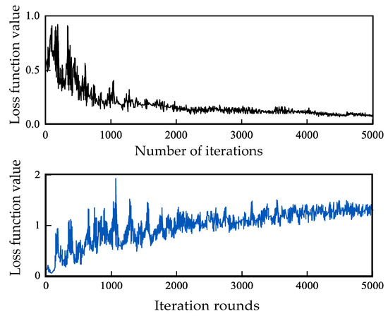
Figure 6.
Loss function value variations.
To visualize the distribution differences between the generated and real samples, the relative errors of the mean and standard deviation of each characteristic item in the velocity structure function generation set and the training set were computed. Figure 7 shows that the relative errors of the mean value of the feature items in the dataset laid mostly within 6%, indicating that the generated samples closely matched the true sample distribution; these verification results were considered good [25].
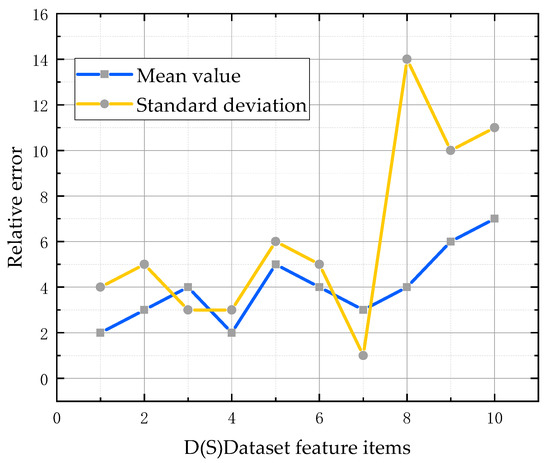
Figure 7.
Relative errors of the generated and training sets.
The relative errors of the standard deviation were generally large, mainly concentrated in three groups. This was caused by the small standard deviation of the training sample set and the large standard deviation of the generated sample set. However, from the perspective of sample diversity, the differences between the generated samples and training samples could enrich the sample diversity to a certain extent and reasonably increase the number of samples. This improved the subsequent model’s classification performance.
The CGAN model was used to expand the mild, moderate, and severe turbulence data in the original dataset to 16,000 samples each. Table 5 shows a comparison among the data volumes of the three turbulence types before and after performing sample expansion. After using the CGAN model for data expansion, the sample ratio of each category in the expanded sample set reached equilibrium.
Table 5.
Comparison among the data volumes of different categories before and after expansion.
During the CGAN model training process, the output of the discriminator could use both the sigmoid function and the softmax function to accomplish different tasks simultaneously. One task was to determine the authenticity of the output sample through the fully connected layer and the sigmoid function. The other task was to generate classification results using the fully connected layer and the softmax function. Compared to neural network classifiers, XGBoost classifiers could achieve a powerful learning ability through multiple weak models to accomplish learning tasks more effectively. XGBoost classifiers could better address the recognition accuracy and speed issues of model recognition and classification, particularly when facing massive and high-dimensional velocity structure function samples. Ultimately, this led to high-performance outcomes. Therefore, after combining the generated samples generated by the CGAN model with the real samples, an augmented sample set was built to train the XGBoost algorithm. The model’s hyperparameters were optimized using a grid search methodology.
Table 6 displays the XGBoost parameters. The learning rate had a value of 0.01, which controls the operational efficiency and accuracy of the model. The number of trees used for classification was set to 150, indicating the maximum number of classifier iterations. The L1 and L2 regularization terms for the weight controlled the regularization part of the classifier and were both set to 1 to reduce overfitting. The minimum sample weight sum value for the leaf nodes was 5, determining the minimum number of classifier node samples. The maximum depth of the tree, which was controlled to avoid overfitting, was set to 6. The descent value of the minimum loss function required for classifier node splitting was 0.1. To evaluate the performance of the CGAN-generated augmented sample set yielded by the CGAN-XGBoost turbulence recognition and classification model, the XGBoost model was trained using both the original dataset and the reconstructed augmented sample set and tested on the test set. The experimental results indicated that the accuracy of this model was 0.89, which was a 15% increase over that of the model trained on the original dataset alone. The comparative test results obtained on the original dataset and the expanded sample set are displayed in Table 7. After expanding the moderate and severe turbulence samples, the accuracy and recall rates achieved for these two rare types of turbulence were significantly improved by this model. This suggested that the model could identify moderate and severe levels of turbulence more effectively than the model obtained before sample expansion. The precision value of the moderate turbulence category increased from a maximum of 0.44 to 0.77, while the recall value also increased from a maximum of 0.40 to 0.83. The severe turbulence category experienced a significant improvement, with the precision value increasing from 0.20 to 0.73 and the recall value increasing from 0.27 to 0.82.
Table 6.
XGBoost parameter settings.
Table 7.
Comparison results of the test conducted on the original dataset and the augmented sample set.
When using the original dataset, the precision and recall values produced for the moderate and severe turbulence categories were typically low. This was caused by the low proportions of these categories in the dataset and the classifier’s inability to fully learn their distinctive features; as a result, the model had difficulty accurately identifying and classifying these categories. By expanding the proportions of rare class samples, the classifier could learn their features more effectively. This would allow the model to better identify the rare class samples, particularly the moderate and severe turbulence categories, resulting in a significant recognition accuracy improvement.
3.2. Method Comparison
Deep learning is widely used in various fields. Alireza Taheri Dehkordi et al. [26] used generated samples to train support vector machines and random forest models for water body mapping. Linsheng Huang et al. [27] used a random forest algorithm combined with the extreme gradient enhancement method to detect early and middle wheat stripe rust. Rajdeep Ghosh et al. [28] automatically detected and removed blinking and muscle artifacts in EEG data by using the k-nearest neighbours (KNN) classifier and a long short-term memory (LSTM) network. To verify the recognition and classification performance of XGBoost in the proposed model, traditional classification algorithms such as KNN, SVM, and RF models were selected and compared with the classification model developed in this paper to assess its effectiveness. KNN is a concise and effective classic classification method that determines a sample’s category by considering the category of its nearest neighbouring sample. An SVM can reasonably partition the hyperplane of the categories in a dataset and handle nonlinear classification problems using kernel functions. The RF model and XGBoost are both types of integrated learning methods that obtain the final classification results through simple voting according to the classifications of multiple base classifiers. These algorithms have high accuracy and generalization capabilities and perform well in both classification and regression tasks.
When modelling each algorithm, a grid search was used to traverse the combinations of different parameter values to find the optimal hyperparameter combination that ensured optimal performance. Then, the three traditional models were trained using the same reconstructed augmented sample set, and the best parameter combination was selected as the final parameter set of each algorithm based on the performance achieved on the test set.
To evaluate the classification accuracies of various algorithms with respect to identifying different levels of turbulence, the harmonic average F1 value was generally used. The F1 value comprehensively considered both accuracy and recall in classification evaluations. A comparison among the F1 values produced by the four algorithms for the three types of turbulence is displayed in Figure 8.

Figure 8.
F1 values produced by different classifiers for each category.
The XGBoost model achieved F1 values of 0.93, 0.80, and 0.77 for the three turbulence categories. The RF model achieved F1 values of 0.91, 0.78, and 0.74. The SVM model achieved F1 values of 0.86, 0.79, and 0.72. The KNN model achieved F1 values of 0.78, 0.71, and 0.68. In terms of classification, the F1 values of XGBoost were higher than those of the other three traditional models for the three turbulence categories. Figure 9 shows a model performance comparison among the four algorithms on the test set based on the same augmented sample set. The accuracy rate of XGBoost was 0.89, with an accuracy rate of 0.81, a recall rate of 0.85, and an F1 value of 0.83. The results indicated that the average performance indicators of XGBoost were significantly superior to those of the other algorithms.
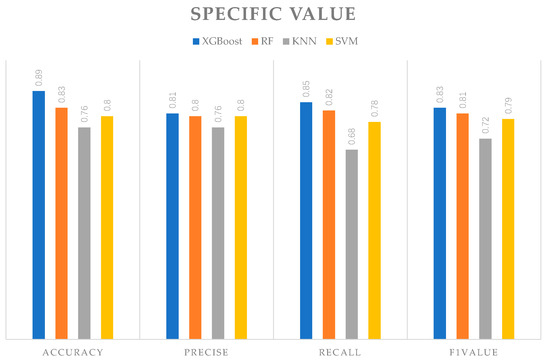
Figure 9.
Model performance comparison among different classifiers.
The wind field data obtained from the LiDAR system and the prediction and recognition results of the four models were compared and analysed. First, the measured data were input into each model to obtain turbulence identification and classification results. Then, the traditional VSF method was used to calculate the actual turbulence intensity value from the measured data, and the spatial distribution results of the cube root of the EDR in the corresponding region were obtained. Finally, the classification results output by EDR1/3 and each model were compared. The spatial distribution results of EDR1/3 are displayed in Figure 10. The vertical axis represents EDR1/3, while the horizontal and vertical axes represent the scanning azimuth and distance gate positions, respectively. The scanning azimuth and distance gate positions are separated by 30° and 300 m per unit, respectively. The horizontal and vertical intervals in each unit constitute 36 sector regions.
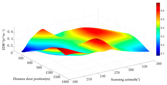
Figure 10.
Spatial distribution of the EDR.
The classification results of each model and the actual values of each region calculated by the velocity structure function method were statistically analysed. Table 8 shows a statistical comparison among the four models and some actual values (omitting the identification consistency levels of the four methods). In the table, H, M, and L represent the high, middle, and low levels of classified turbulence, respectively. The classification results predicted by each model were sequentially compared with the actual EDR calculated by VSF, and a total of 36 comparisons were completed to determine the recognition accuracy of each model prediction. The experimental results indicated that the recognition accuracy of the proposed model was 83%, and the number of false positives in the 36 comparisons was 6. Among the other models, the recognition accuracy of the KNN model was 69% with 11 false positives, while the recognition accuracy of the SVM model was 75% with 9 false positives. The recognition accuracy of the RF model was 78%, with 8 false positives. This paper’s model had the fewest false positives and performed better than the other three methods by 14%, 8%, and 5%, respectively, with superior prediction accuracy.
Table 8.
Comparison between the results of 4 models and the actual VSF values.
3.3. Comparison and Analysis of Flight Crew Reports
To verify the overall practical ability of the CGAN-XGBoost model in terms of identifying turbulence, experiments were conducted by applying the model to real wind fields and comparing the results with flight crew reports. Crew reports contain information about the dates, times, locations (latitudes, longitudes, and flight altitudes), types, and severity levels of the encountered turbulence. They are widely used in research for understanding and predicting various aviation weather phenomena, and they serve as an important basis for identifying and comparing atmospheric turbulence levels. This article included flight crew reports produced for relevant flights at Lanzhou Zhongchuan Airport that encountered turbulence in the airport’s near-air area from January 2018 to June 2019. Based on the times and locations of the turbulence encountered in 18 flight crew reports, the detection data of the LiDAR system that were closest to and at the same locations at the same time were identified and input into the model for identification to verify the overall model application effect. The comparison between the model identification results and the flight crew reports is presented in Figure 11.
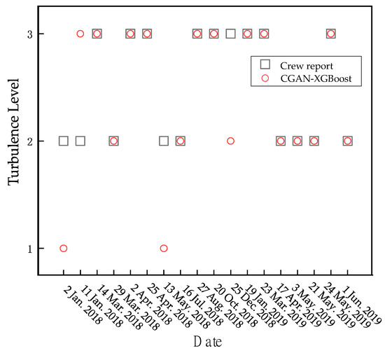
Figure 11.
Comparison between the CGAN-XGBoost identification results and the crew reports.
On the longitudinal axis, Y = 1 indicates slight turbulence, Y = 2 indicates moderate turbulence, and Y = 3 indicates severe turbulence; the abscissa represents the date on which the unit reported experiencing turbulence. The comparison with the crew reports indicates that the proposed model produces a total of four incorrect classification judgements, resulting in a recognition hit rate of 78% for turbulence. Two of the false judgements occur for 5 January and 13 May. The unit reported experiencing moderate turbulence, which the model judges as mild turbulence. On 25 December, the unit reported experiencing severe turbulence, but the model classifies it as moderate turbulence. These three errors are considered false positives produced by the model, resulting in a false-positive rate of 16.7%. Additionally, on 11 January, the unit reported experiencing moderate turbulence, but the model’s classification result is severe turbulence. This judgement is a false alarm, resulting in a false-alarm rate of 5.6%.
In order to make the recognition results more clearly displayed, Figure 12 adds a confusion matrix to the model recognition results. Based on the 18 comparative crew report experiments, these results indicate that the model has a high recognition hit rate for identifying turbulence and can effectively identify turbulence.

Figure 12.
Confusion matrix of CGAN XGBoost recognition results.
4. Discussion
An aircraft flight report represents a real wind shear situation. This paper collected Lanzhou Zhongchuan Airport flight reports dated from January 2018 to June 2019 to verify the effectiveness of the CGAN-XGBoost model proposed in this paper for turbulence identification. In this dataset, 60 groups of wind shear data and 48 groups data without wind shear from the flight reports were used. In this paper, the azimuth interval between the adjacent radial lines of the radar was 5°, and the distance from the gate was 30 m. The whole process involved calculating and obtaining the velocity structure function values of different distances to form a dataset through data preprocessing. Through training on the training samples, the correction of the loss function was of great significance for the training process, as it not only prevented the model from overfitting but also prevented the model from underfitting while ensuring the generalization performance of the model. The new model underwent a total of 5000 iterations of training. The results showed that the model converged after 2000 rounds of training. After 5000 rounds of training, the loss function value tended to become stable, indicating that the model at this time reached the final equilibrium point. During the iteration process, the relative errors of the feature mean in the dataset were mostly within 6%.
In this paper, the new method was mainly compared with the traditional KNN, SVM, and RF approaches. In most cases, the accuracy rate P, recall rate R, and average F1 value were used to evaluate the performance of various algorithm. Therefore, during the comparison process, this paper mainly used the above parameters to evaluate the classification effect of the model. Through experiments, it could be obtained that the F1 values of the XGBoost model for the three turbulence categories were 0.93, 0.80, and 0.77. Those of the RF model were 0.91, 0.78, and 0.74. Those of the SVM model were 0.86, 0.79, and 0.72. Those of the KNN model were 0.78, 0.71, and 0.68. The average performance indicators obtained by the new model on this dataset were significantly better than those of the other algorithms.
Subsequently, this article also calculated the VSF and EDR values for comparison purposes, completing a total of 36 comparisons. Finally, the recognition accuracy of each model prediction was obtained. The experimental results showed that the recognition accuracy of the proposed model was 83%, and the number of false positives out of the 36 comparisons was 6. Among the other models, the recognition accuracy of the KNN model was 69%, and the number of false positives was 11; the recognition accuracy of the SVM model was 75%, and the number of false positives was 9; the recognition accuracy of the RF model was 78%, and the number of false positives was 8. The model in this article had the least number of false positives, and its performance improved by 14%, 8%, and 5% over the other three methods. The experiment showed that the new model had higher recognition and prediction accuracy than other models.
Among the flight crew reports, the proposed model produced a total of four incorrect classification judgments, with a turbulence recognition hit rate of 78%. Three of the erroneous judgments were considered false positives, yielding a false-positive rate of 16.7%. The model provided one false alarm for turbulence, with a false-alarm rate of 5.6%. In summary, it could be seen that the new model could effectively identify turbulence with high accuracy and stability.
5. Conclusions
The use of a CGAN effectively addressed the low recognition and classification performance caused by imbalanced numbers of turbulence category samples in the given dataset and direct modelling. By generating several categories of turbulence samples that matched the distribution of the original data, the recognition and classification performance of the developed model was improved. The XGBoost algorithm was used to further improve the recognition and classification accuracy attained for the massive, high-dimensional, augmented sample sets generated by the CGAN, ultimately achieving high-performance results. Through the study of flight turbulence levels, a flight turbulence recognition model based on CGAN-XGBoost was constructed. This model made it possible to automatically recognize turbulence based on LiDAR.
- (1)
- The performance achieved on the augmented sample set generated by CGAN in terms of identifying the moderate and severe turbulence categories was shown to be good. This was tested by training and testing the XGBoost model on both the original dataset and the augmented sample set. This demonstrated the practical application of the proposed model.
- (2)
- To verify the classification performance of XGBoost and the overall model’s ability to recognize turbulence, three benchmark models were selected, namely, the KNN, SVM, and RF algorithms. These algorithms were compared with XGBoost to characterize their classification performance. The performance of XGBoost was validated using measured wind speed data and was proven to be optimal.
- (3)
- The model was compared and validated using flight crew reports collected from Lanzhou Zhongchuan Airport. The results showed that the model had a recognition hit rate of 78%, a false-positive rate of 16.7%, and a false-alarm rate of 5.6%. These results demonstrate that the developed model had a good ability to identify flight turbulence.
Author Contributions
Conceptualization, Z.Z., H.Z., P.-W.C., H.T. and Z.D.; methodology, Z.Z., H.Z., P.-W.C. and Z.D.; software, Z.Z. and Z.D.; validation, Z.Z., H.Z. and P.-W.C.; formal analysis, Z.Z., H.Z., H.T. and Z.D.; investigation, Z.Z. and H.Z.; resources, P.-W.C.; data curation, Z.Z. and P.-W.C.; writing—original draft preparation, Z.Z.; writing—review and editing, H.Z., H.T. and P.-W.C.; visualization, Z.Z., H.Z., H.T. and P.-W.C.; supervision, H.Z., P.-W.C. and H.T.; project administration, H.Z. and Z.D.; funding acquisition. All authors have read and agreed to the published version of the manuscript.
Funding
This research is funded by the National Natural Science Foundation of China (grant number U2033207), the Natural Science Foundation of Tianjin, China (grant number 21JCYBJC00740) and Key Research and Development-Social Development Program of Jiangsu Province, China (No. BE2021685).
Institutional Review Board Statement
Not applicable.
Informed Consent Statement
Not applicable.
Data Availability Statement
Not applicable.
Conflicts of Interest
The authors declare no conflict of interest.
References
- Gimmestad, G.; Roberts, D.; Stewart, J.; Wood, J. Development of a lidar technique for profiling optical turbulence. Opt. Eng. 2012, 51, 101713. [Google Scholar] [CrossRef]
- Chan, P.W. LIDAR-based turbulence intensity calculation using glide-path scans of the Doppler LIght Detection And Ranging (LIDAR) systems at the Hong Kong International Airport and comparison with flight data and a turbulence alerting system. Meteorol. Z. 2010, 19, 549–563. [Google Scholar] [CrossRef]
- Chan, P.W.; Shao, A.M. Depiction of complex airflow near Hong Kong International Airport using a Doppler LIDAR with a two-dimensional wind retrieval technique. Meteorol. Z. 2007, 16, 491–504. [Google Scholar] [CrossRef]
- Liu, Z.L.; Barlow, J.F.; Chan, P.-W.; Fung, J.C.H.; Li, Y.G.; Ren, C.; Mak, H.W.L.; Ng, E. A Review of Progress and Applications of Pulsed Doppler Wind LiDARs. Remote Sens. 2019, 11, 2522. [Google Scholar] [CrossRef]
- Kim, S.-H.; Kim, J.; Kim, J.-H.; Chun, H.-Y. Characteristics of the derived energy dissipation rate using the 1 Hz commercial aircraft quick access recorder (QAR) data. Atmos. Meas. Tech. 2022, 15, 2277–2298. [Google Scholar] [CrossRef]
- Boilley, A.; Mahfouf, J.-F. Wind shear over the Nice Côte d’Azur airport: Case studies. Nat. Hazards Earth Syst. Sci. 2013, 13, 2223–2238. [Google Scholar] [CrossRef]
- Pichugina, Y.L.; Tucker, S.C.; Banta, R.M.; Brewer, W.A.; Kelley, N.D.; Jonkman, B.J.; Newsom, R.K. Horizontal-Velocity and Variance Measurements in the Stable Boundary Layer Using Doppler Lidar: Sensitivity to Averaging Procedures. J. Atmos. Ocean. Technol. 2008, 25, 1307–1327. [Google Scholar] [CrossRef]
- Ahijevych, D.; Pinto, J.O.; Williams, J.K.; Steiner, M. Probabilistic Forecasts of Mesoscale Convective System Initiation Using the Random Forest Data Mining Technique. Weather Forecast. 2016, 31, 581–599. [Google Scholar] [CrossRef]
- Muñoz-Esparza, D.; Sharman, R.D.; Deierling, W. Aviation Turbulence Forecasting at Upper Levels with Machine Learning Techniques Based on Regression Trees. J. Appl. Meteorol. Clim. 2020, 59, 1883–1899. [Google Scholar] [CrossRef]
- Zhang, J.C.; Zhao, X.W. Spatiotemporal wind field prediction based on physics-informed deep learning and LIDAR measurements. Appl. Energy 2021, 288, 116641. [Google Scholar] [CrossRef]
- Mizuno, S.; Ohba, H.; Ito, K. Machine learning-based turbulence-risk prediction method for the safe operation of aircrafts. J. Big Data 2022, 9, 29. [Google Scholar] [CrossRef]
- Duraisamy, K.; Iaccarino, G.; Xiao, H. Turbulence Modeling in the Age of Data. Annu. Rev. Fluid Mech. 2019, 51, 357–377. [Google Scholar] [CrossRef]
- Subramaniam, A.; Wong, M.-L.; Borker, R.; Nimmagadda, S.; Lele, S. Turbulence enrichment with physics-informed generative adversarial network. In Proceedings of the Neural Information Processing Systems, Online, 6–12 December 2020. [Google Scholar]
- Wang, C.Y.; Deng, C.; Wang, S.Z. Imbalance-XGBoost: Leveraging weighted and focal losses for binary label-imbalanced classification with XGBoost. Pattern Recognit. Lett. 2020, 136, 190–197. [Google Scholar] [CrossRef]
- Purohit, S.; Ng, E.Y.K.; Kabir, I. Evaluation of three potential machine learning algorithms for predicting the velocity and turbulence intensity of a wind turbine wake. Renew. Energy 2021, 184, 405–420. [Google Scholar] [CrossRef]
- Liu, J.; Xu, K.Z.; Cai, B.G.; Guo, Z.B. Fault Prediction of On-Board Train Control Equipment Using a CGAN-Enhanced XGBoost Method with Unbalanced Samples. Machines 2023, 11, 114. [Google Scholar] [CrossRef]
- Jia, J.-F.; Chen, X.-Z.; Bai, Y.-L.; Li, Y.-L.; Wang, Z.-H. An interpretable ensemble learning method to predict the compressive strength of concrete. Structures 2022, 46, 201–213. [Google Scholar] [CrossRef]
- Peña, A.; Mann, J. Turbulence Measurements with Dual-Doppler Scanning Lidars. Remote Sens. 2019, 11, 2444. [Google Scholar] [CrossRef]
- Wildmann, N.; Päschke, E.; Roiger, A.; Mallaun, C. Towards improved turbulence estimation with Doppler wind lidar velocity-azimuth display (VAD) scans. Atmos. Meas. Tech. 2020, 13, 4141–4158. [Google Scholar] [CrossRef]
- Dellwik, E.; Mann, J.; Bingöl, F. Flow tilt angles near forest edges—Part 2: Lidar anemometry. Biogeosciences 2010, 7, 1759–1768. [Google Scholar] [CrossRef]
- Goodfellow, I.; Pouget-Abadie, J.; Mirza, M.; Xu, B.; Warde-Farley, D.; Ozair, S.; Courville, A.; Bengio, Y. Generative Adversarial Networks. Commun. ACM 2020, 63, 139–144. [Google Scholar] [CrossRef]
- Liu, X.B.; Qiao, Y.L.; Xiong, Y.H.; Cai, Z.H.; Liu, P. Cascade conditional generative adversarial nets for spatial-spectral hyperspectral sample generation. Sci. China Inf. Sci. 2020, 63, 140306. [Google Scholar] [CrossRef]
- Rehman, S.; Mohandes, M.A.; Alhems, L.M. Wind speed and power characteristics using LiDAR anemometer based measurements. Sustain. Energy Technol. Assess. 2018, 27, 46–62. [Google Scholar] [CrossRef]
- Shu, Z.R.; Li, Q.S.; He, Y.C.; Chan, P. Observations of offshore wind characteristics by Doppler-LiDAR for wind energy applications. Appl. Energy 2016, 169, 150–163. [Google Scholar] [CrossRef]
- Oh, J.-H.; Hong, J.Y.; Baek, J.-G. Oversampling method using outlier detectable generative adversarial network. Expert Syst. Appl. 2019, 133, 1–8. [Google Scholar] [CrossRef]
- Taheri Dehkordi, A.; Valadan Zoej, M.J.; Ghasemi, H.; Ghaderpour, E.; Hassan, Q.K. A New Clustering Method to Generate Training Samples for Supervised Monitoring of Long-Term Water Surface Dynamics Using Landsat Data through Google Earth Engine. Sustainability 2022, 14, 8046. [Google Scholar] [CrossRef]
- Huang, L.; Liu, Y.; Huang, W.; Dong, Y.; Ma, H.; Wu, K.; Guo, A. Combining Random Forest and XGBoost Methods in Detecting Early and Mid-Term Winter Wheat Stripe Rust Using Canopy Level Hyperspectral Measurements. Agriculture 2022, 12, 75. [Google Scholar] [CrossRef]
- Ghosh, R.; Phadikar, S.; Deb, N.; Sinha, N.; Das, P.; Ghaderpour, E. Automatic Eyeblink and Muscular Artifact Detection and Removal from EEG Signals Using k-Nearest Neighbor Classifier and Long Short-Term Memory Networks. IEEE Sens. J. 2023, 23, 5422–5436. [Google Scholar] [CrossRef]
Disclaimer/Publisher’s Note: The statements, opinions and data contained in all publications are solely those of the individual author(s) and contributor(s) and not of MDPI and/or the editor(s). MDPI and/or the editor(s) disclaim responsibility for any injury to people or property resulting from any ideas, methods, instructions or products referred to in the content. |
© 2023 by the authors. Licensee MDPI, Basel, Switzerland. This article is an open access article distributed under the terms and conditions of the Creative Commons Attribution (CC BY) license (https://creativecommons.org/licenses/by/4.0/).