Atmospheric CH₄ and Its Isotopic Composition (δ¹³C) in Urban Environment in the Example of Moscow, Russia

Abstract

Measurements of near-surface methane (CH₄) mixing ratio and its stable isotope ¹³C were carried out from January 2018 to December 2020 at the A.M. Obukhov Institute of Atmospheric Physics (IAP) research site in the center of Moscow city. The data show moderate interannual variations in monthly mean CH₄ with maximum values being observed predominantly in winter (2.05–2.10 ppmv on average). The most δ¹³C depleted CH₄ (up to −56‰) is observed in summer and autumn following seasonal decrease in traffic load in the city. The highest CH₄ concentrations (>2.2 ppmv) were likely to be caused by air transport from the E–SE sector where potentially large microbial CH₄ sources are located (landfills and water treatment plants, Moscow River). Keeling plots of these episodes in different seasons of 2018–2020 showed δ¹³C isotopic signatures of about −58–−59‰ for the spring–autumn period and −67‰ for winter. A good correlation was observed between CH₄ and other pollutants: CO₂, CO, and benzene in daytime (10:00–19:00) hours (R > 0.7). Contribution of urban methane emissions due to vehicle exhausts (∆[CH₄]_auto) and microbial activity (∆[CH₄]_micro+) along with regional baseline mixing ratios of CH₄ ([CH₄]_base) and CO ([CO]_base) were estimated from the linear orthogonal regression analyses of the measured daytime mixing ratios. A significant role of microbial methane in the formation of CH₄ maximums in Moscow was revealed. Contributions of the upwind continental CH₄ and CO sources to the measured species levels were estimated through comparison with the Mace Head site data representative for the Northern Hemisphere baseline air. The study provides, for the first time, important insights into the long- and short-term variations of CH₄ levels in Moscow in connection to the local (urban) emissions and long-range transport from upwind continental sources. The results will contribute to elaboration of a default emission inventory in air quality modeling and help to identify the areas for targeted mitigation efforts.

1. Introduction

Methane (CH₄) is the second most abundant anthropogenic greenhouse gas after carbon dioxide (CO₂), affecting the Earth’s atmospheric heat balance and chemistry [1]. Urban environments produce about 70% of anthropogenic greenhouse gas emissions and 21% of global CH₄ emissions [2]. The latter are attributed mainly to transportation (~43% of the total urban emissions), energy (~42%), waste (~40%), and agriculture (~5%) [3].

Urban population growth accompanied by increase in urban-occupied territories and anthropogenic loading requires better understanding of the contribution of urban CH₄ to global emissions. Cities are equipped with variable facilities that represent widespread sources of methane, including landfill sites, gas storage and distribution networks, wastewater plants, heating systems and vehicles, and water treatment plants [4,5,6]. The relative contribution of the above sources can vary greatly from city to city which creates a need for employing long-term observation systems to assess contribution of individual sources for a particular urban environment.

The results of direct measurements and chemical transport simulation are the basis for the solutions on urban air pollution abatements. However, there are large uncertainties in urban CH₄ budgets, as mentioned in a substantial number of studies (see [1,2,7,8] and references therein). CH₄ inventories tend to underestimate emissions compared to those inferred from direct atmospheric measurements of methane levels due to difficulty in correctly accounting for fugitive CH₄ emissions [9] and the lack of a basic understanding of the locations and temporal patterns of urban CH₄ sources at relevant scales [2]. For example, existing emission estimates for Moscow, inferred from near-surface CH₄ measurements on the Moscow network stations in 2005–2014, show significant inaccuracy of the derived inventories for most chemical compounds [10,11,12]. This strongly supports the need to elaborate new strategies in assessing the urban source strengths for methane and other pollutant species. Yet, long-term monitoring of CH₄ and its urban sources in the city is necessary to identify existing trends and patterns in the data, which is a necessary prerequisite for elaborating effective greenhouse gas abatement strategies.

The source of specific methane emissions can be identified by analyzing the methane isotopic composition, as different source types are characterized by distinct ¹³C signatures (δ¹³CH₄). The isotopic value of a single source category can vary considerably, depending on the CH₄ formation process, geographic origin, season, and secondary alteration [5,13,14]. Thus, the supplementary information about δ¹³CH₄ in urban air is very important.

According to ¹³C measurements in the plums of the main CH₄ sources in urban areas (

Table 1. δ¹³CH₄ from different CH₄ sources.

Source	δ13CH4, ‰	Reference	Location
Biomass burning	−24–−32	[16]	USA (Florida)
	−26.2 ± 4.8	[17]	Hungary (Budapest)
Gas storage sites	−43.4 ± 0.5– −33.8 ± 0.3	[18]	France (Paris)
Natural gas facilities	−41.7 ± 0.7– −49.7 ± 0.7	[15]	Canada (Alberta)
Fossil fuel sources	−15–−45	[17]	Hungary (Budapest)
Gas leaks	−36 ± 2	[4]	Great Britain (London)
Coal mines	−51.2 ± 0.3– −30.9 ± 1.4	[4]	Great Britain (London)
Subarctic wetlands	−68.5 ± 0.7	[10]	Finland (Lompolojänkkä)
Modern microbial sources	−61.7 ± 6.2	[17]	Hungary (Budapest)
Biogenic emissions	−55–−70	[17]	Hungary (Budapest)
Landfills	−55.3 ± 0.2	[15]	Canada (winter)
	−63.7 ± 0.3–−58.2 ± 0.3	[18]	France (Paris)
	−58 ± 3	[4]	Great Britain (London)
	−64.4–−44.3	[11]	Great Britain, Netherlands, Turkey
Aeration station	−53.7 ± 0.1	[11]	Great Britain, Netherlands, Turkey
Oil storage	−54.9 ± 2.9– −60.6 ± 0.6	[18]	France (Paris)

), biogenic and microbial methane (wetlands, landfills, aeration station, water ponds, etc.) as well as methane emitted from oil storages are ¹³C-depleted (δ¹³CH₄: −70 to −50 permils (‰)), while methane from natural gas usage (storage and leaks) and pyrogenic CH₄ (from incomplete combustion of nonfossil organic matter and fossil fuel) are less ¹³C-depleted (δ¹³CH₄: −50 to −30‰ and −30 to −15‰, respectively) [4,10,11,15,16,17,18].

Moscow ranks as the world’s 15th largest city by population and is among the leaders by population density. It is located on the plain in the middle latitudes and has the historically formed urban development with the absence of large industrial centers in the immediate vicinity. This leads to the consideration of Moscow as an isolated city [12]. Over the past 30 years, the number of cars in Moscow has increased from 2 to 6 million and industrial production has increased by 10%. At the same time, the large enterprises contributing to the air pollution stopped working. Thus, Moscow became a financial and administrative center with a composition of anthropogenic emissions similar to cities with the same infrastructure. The main sources of air pollution (motor transport, industrial and communal facilities, housing sector) bring Moscow’s air quality close to the megacities of the USA, Japan, and large European towns [12,19,20].

Regular long-term monitoring of CH₄ and other gases in Moscow and outside of the city has been carried out at the 56 sites of the Moscow Ecological Monitoring (MEM) network since 2002. However, the measurements of CH₄ isotopic composition in Moscow have not carried out.

This study aims to analyze the measurements of surface CH₄ concentration and its stable isotope ¹³C in the center of Moscow city in different seasons of 2018–2020 and to determine the main methane sources. The direct measurements of ¹³CH₄ in the city are carried out for the first time. The study is supposed to provide important insights into the long-term and short-term variations of CH₄ as well as into the sources and dynamics of methane emissions in urban environments.

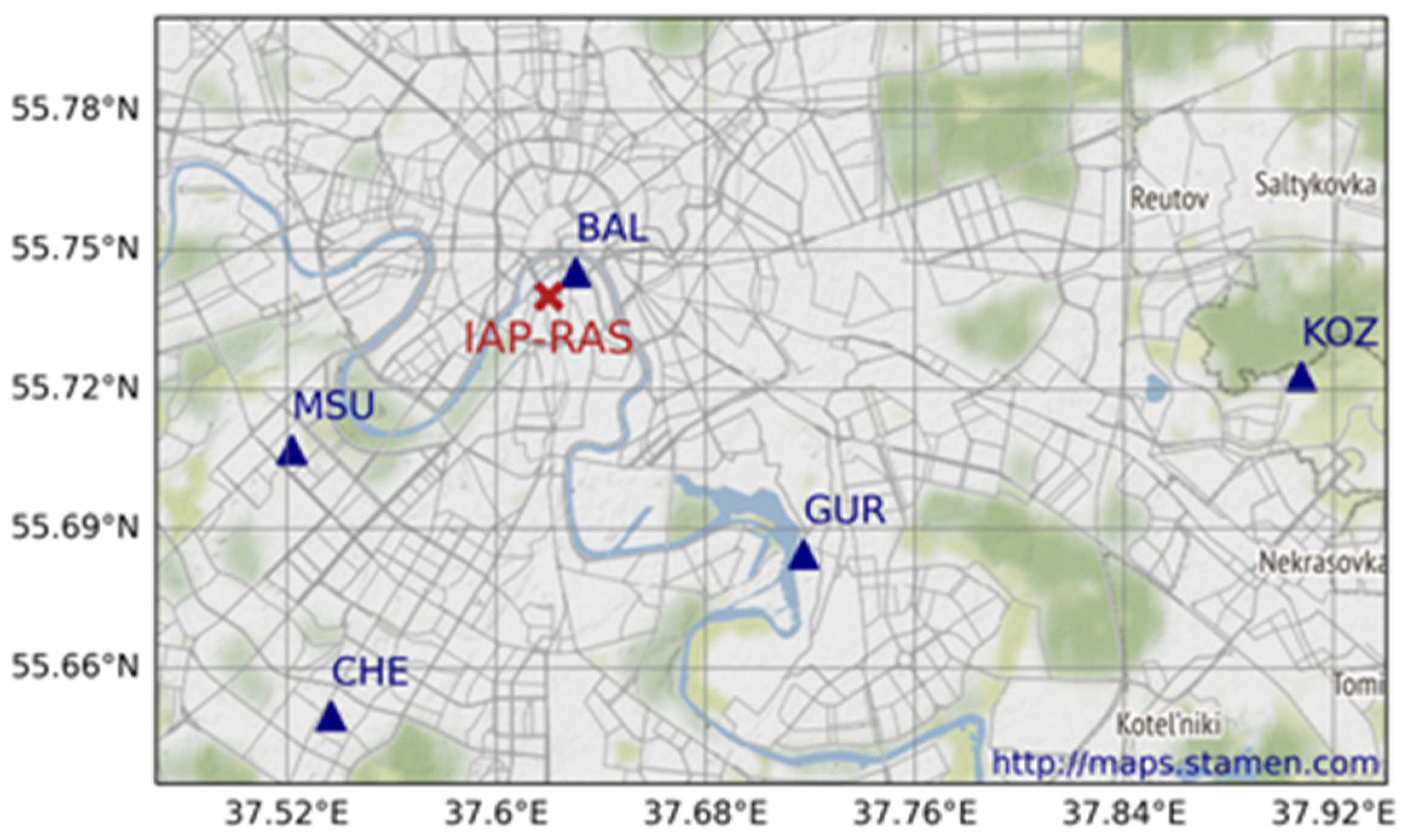
2. Materials and Methods

Measurements of CH₄ mixing ratio and its stable isotope ¹³C as well as CO₂, CO, and benzene mixing ratios were made from January 2018 to December 2020 at the site located at A.M. Obukhov Institute of Atmospheric Physics of the Russian Academy of Sciences (IAP RAS) in the center of Moscow (55°74′ N, 37°62′ E, 130 m a.s.l.). The site is located on a flat terrain, elevation changes do not exceed 3–5 m within a radius of approximately 1 km, and it is surrounded by several low- to moderate-traffic motorways (about 30–40 m away from the site), residential buildings, and business offices up to 20 m in height (Figure 1).

The CH₄ measurements obtained at the IAP RAS site were compared with the data from four urban air quality monitoring sites (Kozhuhovo (KOZ), Guriyanova (GUR), MSU, Cheremushki (BUT)) belonging to the Moscow Ecological Monitoring (MEM) network (https://mosecom.mos.ru/, accessed on 27 February 2023). The MEM network meets the requirements of the World Meteorological Organization for air quality monitoring systems in cities.

To describe the meteorological conditions around the IAP RAS site, meteorological data from the Balchug meteorological station (WMO ID 27605), located ~1 km to the north (55°44 N, 37°37 E, 124 m a.s.l.), were employed. Since variations in topography heights across the Moscow city and adjacent areas are very low (from 120 to 250 m a.s.l.), any differences among the measurements at the IAP RAS site and MEM sites are attributed completely to the spatial variations of the emission sources and (partially) to prevailing wind directions in a particular season.

A completely automatic measurement complex developed at IAP RAS was used for the measurements. Almost all the instruments were placed in all-weather racks, temperature-controlled at +32 °C, and located in open air [21,22] (see Figure S1 in the Supplementary Materials). The CH₄ and δ¹³C were measured with the G2132-i instrument manufactured by Picarro Inc. (Santa Clara, CA, USA) which employed the cavity ring down spectroscopy (CRDS) technique. The instrument has a measurement range of 1.8–12 ppmv and a precision of ±0.005 ppmv for methane [23]. Accuracy for δ¹³C is about ±0.8‰. The time resolution of the instrument was about 30 s. Air inlet was the downward funnel located 2.5 m above ground, with PTFE tubing with 1/4″ OD and 3 m length. Air flow via this inlet was maintained at approximately 1.5 L/min (whereas the instrument itself had an air flow less than 0.05 L/min), with an additional pump used to reduce the transit time from the air inlet to the instrument.

This instrument was earlier used by the present authors to measure methane mixing ratio and δ¹³C onboard the research vessel in the Arctic [24,25]. All the measurements showed a good reliability of the instrument, with no faults or malfunctioning having occurred.

The instrument was first calibrated with the secondary standard which was a 1 L compressed air cylinder with known concentrations of methane and δ¹³C provided by the Norwegian Institute for Air Research (NILU). That secondary standard was calibrated in NILU by the primary standard known as NOAA04 [26] for CH₄ and by the method described in [13] for δ¹³C. The relative accuracy for that secondary standard was found to be not exceeding 0.03% for CH₄ and 0.1% for δ¹³C. As a result of calibration by that secondary standard, the calibration correction factor for the instrument was thus defined. Then, the calibrated instrument was used to measure true concentrations in cylinders with gas standards provided by Linde Gas Rus company (Balashikha, Russia) with a significantly better accuracy (Table S1), namely about 0.05%, than that of the standards themselves. Subsequently, those gas standards were used to check the long-term stability of the instrument readings, with calibrations carried out in several months’ time intervals. A traditional pneumatic scheme was used for applying gas standard to the instrument at atmospheric pressure, with a rotameter to check vent air flow. The maximum difference in the instrument readings in different calibrations over almost 1.5 years did not exceed 0.005 ppmv, which is within the range of the instrument accuracy declared by the manufacturer (see above). Thus, no additional calibration factors were added. The instrument readings were stable within its declared accuracy. Calibration results are provided in the Supplementary Materials.

Carbon monoxide (CO) concentration was measured using the 48 S instrument provided by Thermo Inc. (Waltham, MA, USA) with a 60 s response time and a range limit of 0.05–10 ppmv. Ozone (O₃) concentration was measured by the 1008-AH instrument provided by Dasibi Inc. (Glendale, CA, USA) with a 60 s response time and a range limit of 1–1000 ppbv.

Benzene was measured by a compact-type proton-transfer-reaction mass spectrometer (PTRMS), provided by Ionicon Analytik GmbH (Innsbruck, Austria) in 2008. To control the instrument and to calculate measured concentrations, the native software PTR-MS Control, version 2.7.1.302, was used. The main principles of PTR-MS operation can be found, for instance, in [23]. The working parameters of PTR-MS operation were the following: primary ions were H₃O+, and E/N = 149.9 Td (1 Td = 10–21 V m²) when Udrift = 600 V, pdrift = 2.0 mbar, and Tdrift = 333 K (60 °C) as default factory values. The levels of impurity ions NO+ (m/z 30), O₂+ (m/z 32), and cluster ions H₃O+(H₂O) (m/z 37) did not exceed 0.1–0.2%, 3–4%, and 0.3–0.4%, respectively, of the primary ion levels during measurements.

The original data were aggregated into 1 h averages provided there were at least 50% valid data measurements in the hour. In the subsequent analysis, the terms winter and summer data refer to the periods of December–February and June–August of 2018–2020, correspondingly. The daytime means (10:00–19:00 local time) of hourly methane, carbon monoxide, carbon monoxide, and benzene mixing ratios for the whole observation period from January 2019 to December 2020, which are further referred to as daytime data, were employed in the correlation analyses. The subset of daily data was considered to be best representative for the average composition of the Moscow air basin as the effect of vertical mixing cannot be clearly separated from other processes contributing to the total species variability at the site.

3. Results

3.1. Meteorology

The whole 2018–2020 observation period is characterized by anomalously warm weather conditions for substantial parts of each season, with highly variable amounts of precipitation for a particular season among different years.

Warm weather and heavy snowfalls persisted in January and February 2018, with air temperature about 5 °C higher in January (Figure 2). Yet, at the end of February 2018, the air temperature dropped below −20° several times. The amount of precipitation in winter exceeded the normal value by more than 1.5 times. The air temperature in spring and autumn 2018 was slightly higher compared to climatological normal for this period. The summer of 2018 was anomalously warm and dry, resulting in total precipitation of 176 mm per season vs. 250 mm of normal value. Warm summer smoothly turned into autumn.

The air temperature and the amount of precipitation in the winter season of 2018–2019 were close to respective climatological normals. Contrarily, the summer months of 2019 were hot and dry, with the amount of precipitation in August being one-third of the climatological normal. The autumn was exceptionally warm and dry as well, with the air temperature ranking the third highest in the history of meteorological observations, and the total precipitation reaching only 67% of its climatological normal.

January 2020 was the warmest year on record in Moscow, with the stable snow cover established only on January 23. The temperatures in Moscow were higher by 2.6 °C in January and 6.3 °C in February 2020 compared to the climatological normals.

The beginning of spring 2020 was warm, but in April–May, the air temperature dropped below the climatological normal. Summer and autumn 2020 were anomalously warm and humid, with the autumn months being the warmest for the whole meteorological observation record in Moscow starting from 1891.

The average 2018–2020 wind speed diagrams for winter and summer months are plotted in Figure 3 for nighttime and daytime hours separately. Low wind speeds of 1 m/s or less obviously prevailed in Moscow in both seasons. The proportion of calm weather conditions was the highest for summer nights (Figure 3a) and the proportion of wind speeds > 3 m/s was the highest in summer daytime hours. There was no significant difference in wind speed between nighttime and daytime in winter (Figure 3b).

3.2. Surface CH₄ and δ¹³C Variation

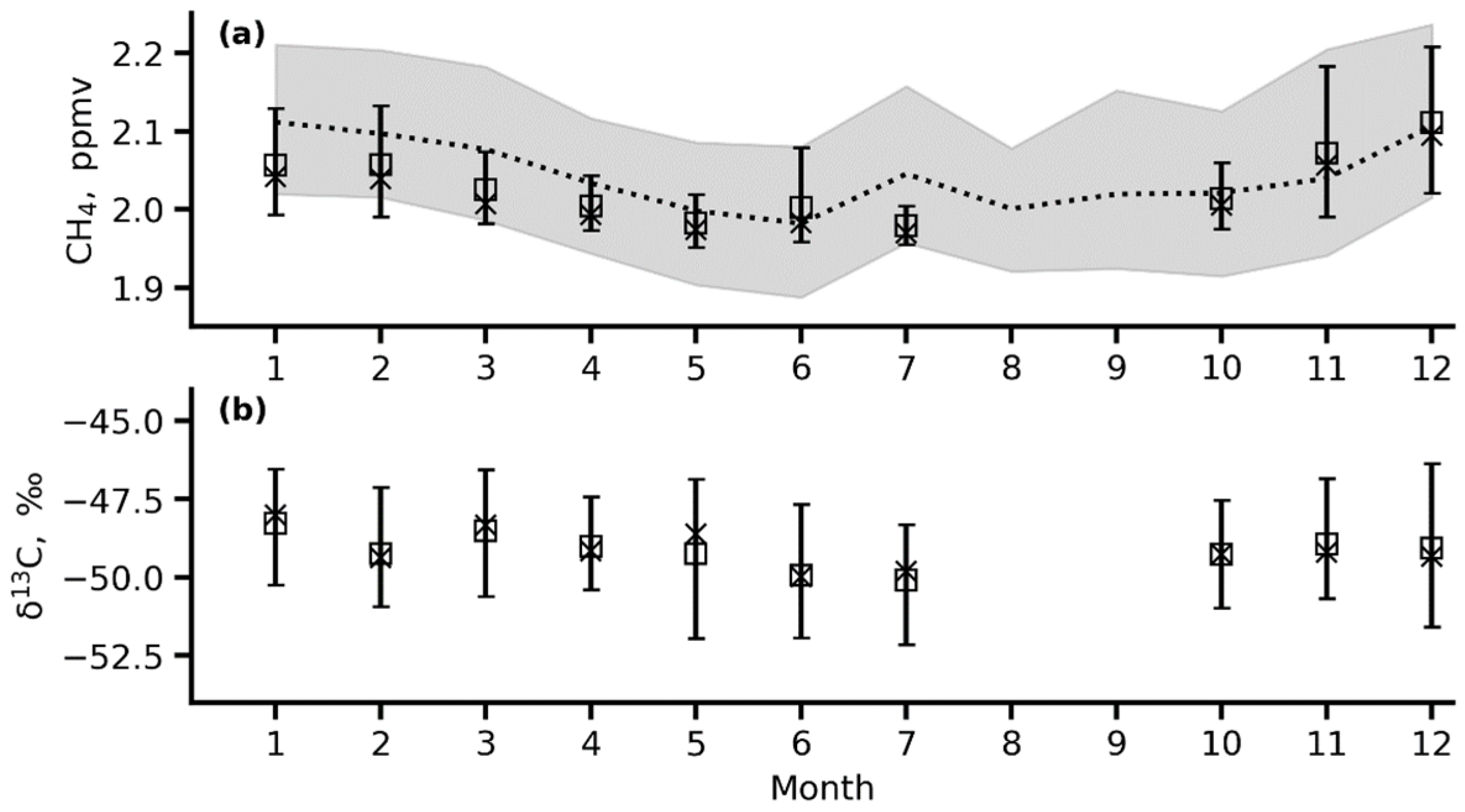
3.2.1. Interannual and Monthly Variations

Interannual variations in monthly mean CH₄ daytime mixing ratios at the IAP RAS site ranged from about 0.05 to 0.1 ppmv. These variations were found to be generally small compared to the amplitude of seasonal cycle (0.15–0.2 ppmv) and total spread of daily values within a particular month (0.05–0.2 ppmv) (Figure 4a,c,e). Maximum CH₄ levels were observed predominantly in winter (2.05–2.10 ppmv on average), reflecting seasonal decrease in methane oxidation date, depth of the mixing layer, and rate of vertical exchange between planetary boundary layer and free troposphere. The highest methane variability on both interyear and seasonal scales was also seen in the cold season due to proportionally higher contribution of distal methane sources via regional and long-range transport processes (see more discussion below in Section 3.4.3).

Relatively small interyear variations in the CH₄ abundance are most probably attributed to the relative stability of the primary urban methane sources affecting the site. The latter conclusion is supported by the similarly moderate interannual variability in the δ¹³C values (Figure 4b,d,f). The most δ¹³C depleted CH₄ is observed in summer of 2018–2019 (−50‰) and in November and December of 2020 (about −50‰ on average). Low δ¹³C values may indicate the predominance of CH₄ emissions from local and remote microbial methane sources (municipal drainage, landfills, aeration station, freshwater reservoirs) in this period of observations.

The IAP RAS CH₄ data show good agreement (R > 0.5) with the CH₄ measurements at the MEM sites in Moscow (Figure 1) as any impacts of heterogeneity of the methane urban emissions are averaged out on a seasonal scale (Figure 4 and Figure 5). The similar consistency was found for the CO and CO₂ data among the IAP RAS and MEM sites notwithstanding substantial spread among the species levels on a particular day or hour. We can conclude, finally, that the IAP RAS site data do provide consistent estimates on the measured species abundances, with the latter being representative at least for the central part of the city.

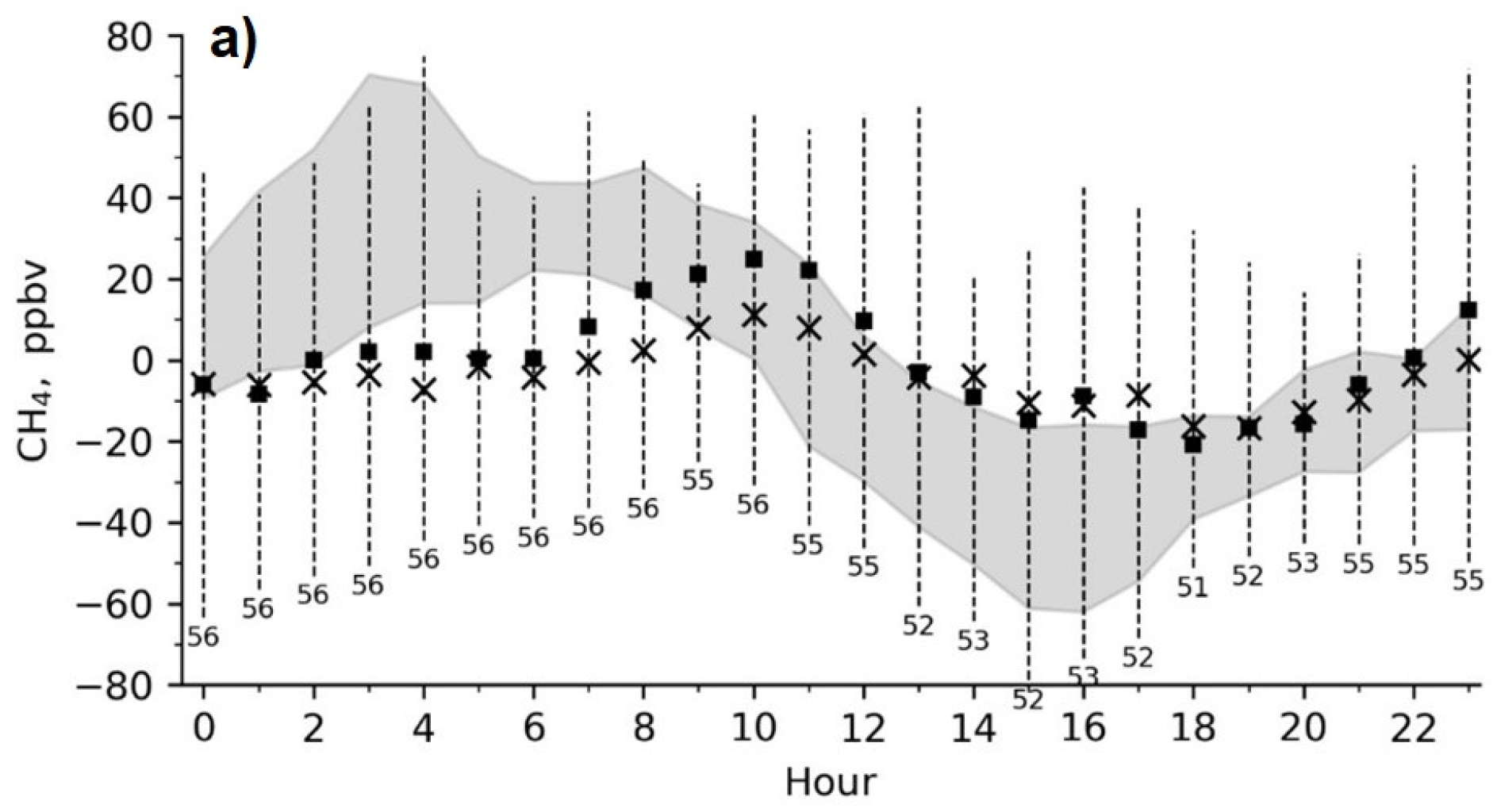
3.2.2. Diurnal Variations

The strength of anthropogenic pollutant sources in Moscow exhibited a weak diurnal dependence and also varied with the day of week [12]. In summer (Figure 6a), CH₄ mixing ratios at the IAP RAS site increased slightly during the nighttime (22:00–07:00) due to accumulation of the CH₄ emissions near the surface, which results in diurnal CH₄ maximum in early morning hours (06:00–08:00) (about 2.2 ppmv) prior to destruction of the nighttime near-surface inversion and entrainment of air from the residual boundary layer.

In winter (Figure 6b), the CH₄ levels were well below 2.2 ppmv with no significant diurnal variations but with a substantial day-by-day variability, as mentioned above. Yet, a weak diurnal variability of CH₄ in winter could appear at some times. The plot of the hourly deviations from the daily CH₄ averages shows an increase in CH₄ values in winter 2018 (Figure 7a) between 08:00 and 12:00. The above feature is distinct in the data and most probably associated with the prevalence of easterly winds in that season and associated CH₄ transport from known industrial facilities located in the east part of the Moscow region. Contrary, the diurnal cycle of CH₄ at the IAP RAS and MEM sites (Figure 7b,c) was very suppressed under prevalence of westerly winds in winter of 2019 and 2020.

Diurnal changes in δ¹³C were insignificant both in summer and in winter, with substantial short-term variations at each hour. The mean δ¹³C values were about −50‰ and −49‰ in summer and winter, correspondingly (Figure 6a,b).

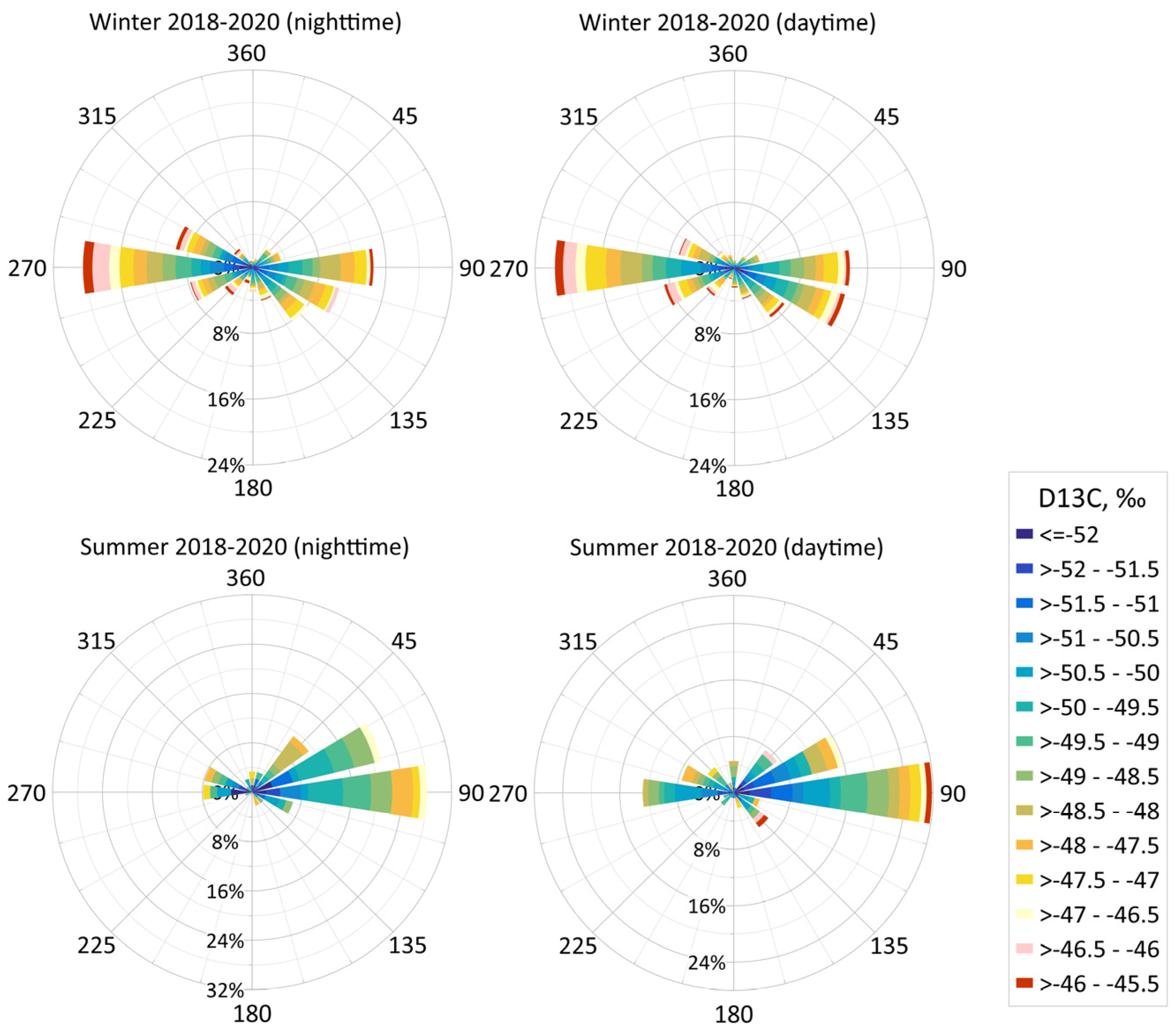
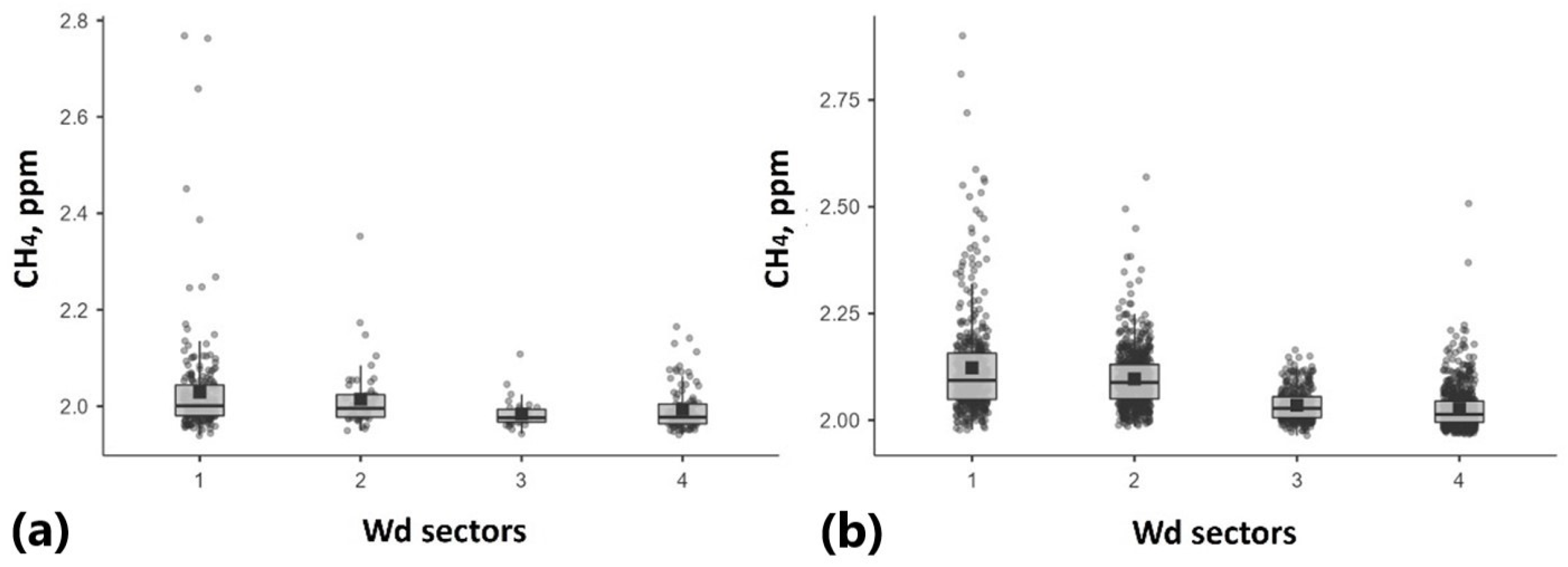
3.3. Impact of Wind Direction

According to Figure 8, the prevailing wind directions are from W and E–SE in winter and from NE–E in summer, with no meaningful separation between the night- and daytime hours. This feature holds for other seasons as well, so the final conclusion is that the easterly winds cause enhanced methane levels at the site throughout the year, which is due to the location of powerful CH₄ anthropogenic sources (natural gas facilities and fossil fuel sources) upwind of the measurement sites in those directions. In summer, methane is more depleted by δ¹³C (Figure 9) and varies generally in a wider range (Figure 10) than in winter. The above features are explained by a comparatively large contribution from microbial CH₄ sources (including remote ones) in warm periods which are also more spatially scattered, similar to other biogenic emissions of minor species, compared to anthropogenic sources.

3.4. Urban CH₄ Sources

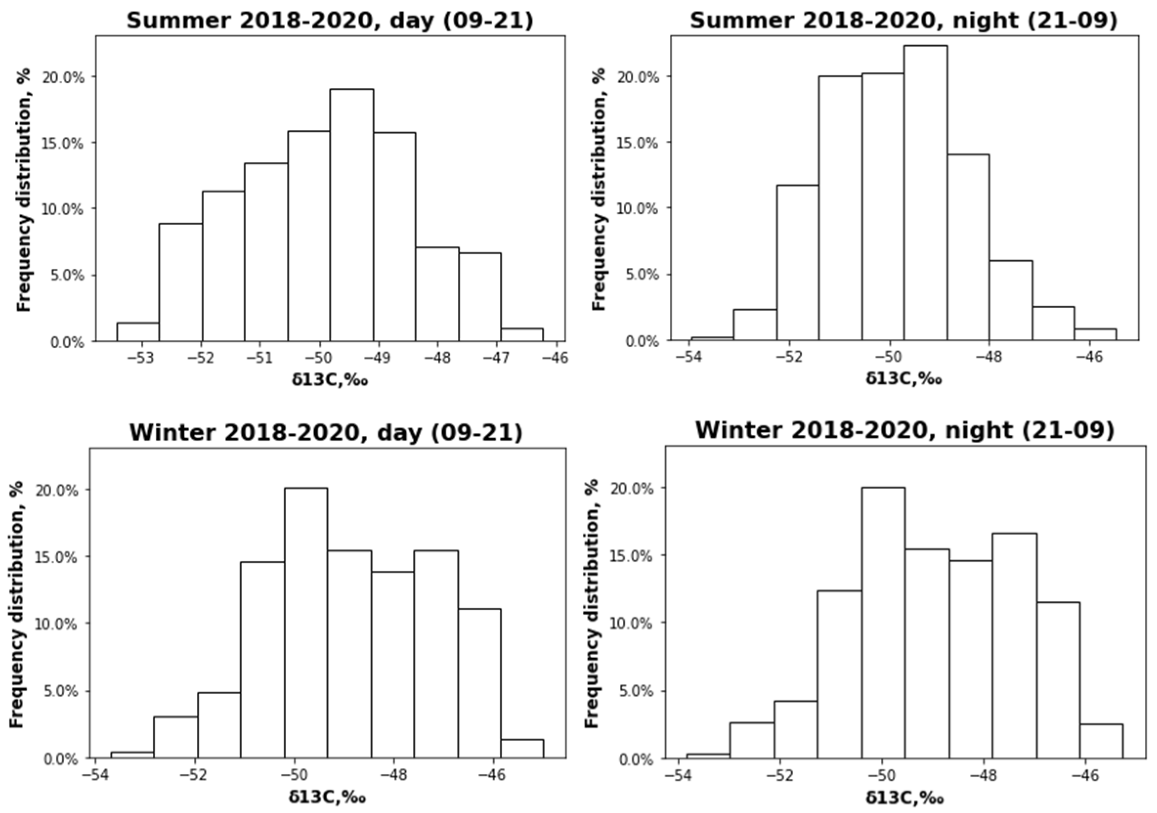
3.4.1. δ¹³CH₄ in Urban Air

Frequency distributions of δ¹³CH₄ for different seasons at night- and daytime hours are shown in Figure 11. In summer, the impact of δ¹³C-depleted CH₄ sources (microbial methane, see Table 1) is more significant than in winter, particularly at nighttime, resulting in δ¹³C values less than −49‰ for more than 50% of measurements. In winter, comparatively larger δ¹³C values are clearly prevailing, with δ¹³C > −50‰ in about 75% of measurements both for night- and daytime data. Such a positive shift also results in a secondary maximum at a δ¹³C value of about −47‰. Clearly, methane emissions associated with fossil fuel and gas usage facilities (vehicle exhausts, natural gas leaks and storage) prove to be the main CH₄ source at the IAP RAS site in a cold season. Yet, the significant δ¹³C peaks at < −50‰ both in summer and winter provide evidence for the important contribution of microbial methane throughout the year.

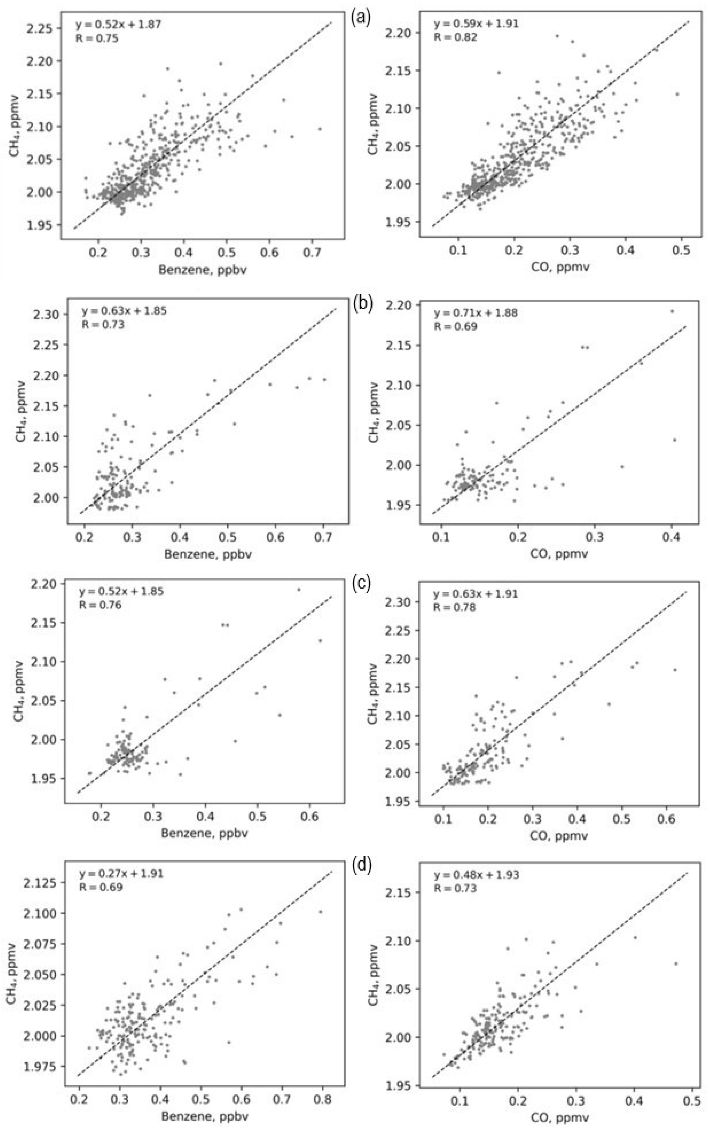
3.4.2. CH₄ Correlation with Other Urban Pollutants

To study the relationships of surface methane with other anthropogenic pollutants, CO₂, CO, and benzene, and to determine the prevailing methane sources, we plotted the orthogonal regression fits for 1 h summertime and wintertime data (Figure 12). The figure shows a good correlation (R > 0.5) between CH₄ and other species, especially in winter (when most of the measurements were made). A high correlation (R ≥ 0.7) was observed between benzene, CO₂, and CO in winter, which points out the shared sources of these gases, namely, vehicle exhausts and thermal power plants. The CH₄ correlates with CO and CO₂ in winter (R ≥ 0.7) better than in summer (R = 0.5–0.6), which highlights the role of fossil fuel sources (mentioned above) in the CH₄ emissions in Moscow in the cold season. However, there are high CH₄ values (hereafter, high-methane episodes) seen mostly as outliers in the scatter plots. The outliers are most probably associated with microbial emissions, as supported by the associated low δ¹³C values (Figure 13). These sources of high methane may be located nearby (drainage, wastewater) as well as a few tens of kilometers away (landfills around the town, water treatment plants, Moscow river), producing spatially coherent atmospheric plumes of the CH₄ reaching air transported to the measurement sites (see more discussion in Section 3.2). Because of the highly episodic nature of high-CH₄ events, we exclude them from the correlation analyses by filtering out the part of the data with [CH₄] > 2.2 ppmv (~2% of the whole dataset). Such simple data filtering was found to be the most effective among the other outlier treatments and results in markedly stable results of the correlation analyses and overall consistency between the CH₄, benzene, and CO data (Figure 14).

3.4.3. Contribution of the Urban CH₄ Sources

We used the simultaneously measured methane (CH₄), carbon monoxide (CO), and benzene (BENZ) mixing ratios to assess the contributions of the urban sources to the measured methane levels through analyses of the daytime [CH4]–[BENZ], [CH4]–[CO], and [CO]–[BENZ] correlations (Figure 14). In the midlatitude troposphere, the chemical lifetime for benzene is relatively short in the summer (~1–2 weeks) but greatly increases in the winter months following a seasonal change in tropospheric hydroxyl abundance [27], causing this compound to be involved in long-range atmospheric transport. Yet, background benzene levels were found to be much lower compared to typical levels in urban air (see, for example, [28] and references therein) as its primary regional sources are strongly connected to spatially localized urban areas with high population density. This allows the use of benzene as a marker of traffic and industry emissions particularly in urban environments. Contrarily, the higher atmospheric lifetime of CO due to lower oxidation rate along with strong contribution of both spatially localized (industrial and biomass burning) emissions and distributed CO sources (due to oxidation of biogenic hydrocarbons and methane) makes it an efficient tracer of polluted air on both regional and hemispheric scales [29].

In our study, we considered enhanced CO and benzene levels as an indicator of the urban air pollution to infer a regional component of the measured methane level. Using daytime (10 a.m.–19 p.m.) mixing ratios of the measured species as representatives for the composition of urban PBL as a whole, one can write the model equations:

[CH₄] = [CH₄]_base + a₁([CO] − [CO]_base),

(1)

[CH₄] = [CH₄]_sum + a₂[BENZ].

(2)

Here, [CH₄]_base and [CO]_base are baseline CH₄ and CO levels, with the respective quantity for [BENZ] assumed to be negligibly small compared to the typical measured urban benzene levels, and [CH₄]_sum represents a sum of [CH₄]_base and ∆[CH₄]_micro+. ∆[CH₄]_micro+ is a contribution of other sources of methane apart from traffic and industry emissions (microbial methane, natural gas and oil storage, natural gas leakages).

Assuming linear (on average over a set of atmospheric conditions) dependence of the atmospheric benzene and CO abundances on their emission rates, the ratio of slope rates a₂/a₁ will be equal to the average BENZ/CO emission ratio for all the pollution sources affecting the urban environment.

We estimate [CH₄]_sum, [CH₄]_base, a₁, and a₂ on a seasonal basis through orthogonal regression of the observed CH₄ mixing ratios ([CH₄]_obs) onto the measured benzene and CO mixing ratios according to Equations (1) and (2). For either Equation (1) or Equation (2), a ratio of standard deviations of the corresponding independent and dependent variables was used as an estimate for the respective ratio of error variances, with the latter being utilized in the standard orthogonal least squares (OLS) procedure.

The seasonal average values [CO]_base were estimated from a subset of ([BENZ], [CO])_obs data points corresponding to the lowest 5% of the observed benzene mixing ratios. This was found to be a reasonable approach, taking into account the lack of any regular CO observations in rural areas around the Moscow town as evidenced from our comparison of the [CO]_base values against available sparse data in the vicinities of the Moscow town obtained during TROICA experiments [30]. Average contributions from vehicle exhausts and industry (∆[CH₄]_auto) and microbial and other activity (∆[CH₄]_micro+) were then estimated as follows:

∆[CH₄]_auto = a₂ ∙ < [BENZ] >,

(3)

∆[CH₄]_micro+ = < [CH₄]_sum–[CH₄]_base >,

(4)

where [∙] marks a value estimated via OLS fit and <∙> represents a seasonal mean. The derived estimate for the regression slope a₂ was found to be well within the range of the reported values for vehicle exhausts [31,32], which can be considered as an independent test for the present estimates for ∆[CH₄]_auto. Our final estimates are summarized in

Table 2. The observed season average CH₄ and CO daytime (10 a.m.–19 p.m.) mixing ratios and estimated contributions of road transport ([CH₄]_auto) and microbial activity ([CH₄]_micro+) at the IAP RAS site. All units are in ppbv for better understanding. Natural variability for [CH₄] and [CO] hourly data along with uncertainty estimates for ∆[CH₄]_auto and ∆[CH₄]_micro+ values is provided as ±1σ (standard deviation) about the mean.

Season	[CH4]	[CO]	∆[CH4]auto	∆[CH4]micro+
Winter	2033 ± 43	206 ± 76	0.17 ± 0.08	40.8 ± 97.9
Spring	2038 ± 53	199 ± 83	0.18 ± 0.09	42.8 ± 124.8
Summer	1992 ± 39	163 ± 56	0.14 ± 0.09	15.9 ± 91.7
Autumn	2013 ± 26	167 ± 54	0.10 ± 0.10	25.9 ± 48.5

, with the standard deviation of each estimate calculated via the error propagation rule [33].

One can see from Table 2 that the regional baseline mixing ratios of CH₄ and CO are subjected to a distinct seasonal cycle with a maximum in winter and a minimum in summer as a result of seasonal changes in atmospheric oxidation power, height of the mixing layer, and vertical exchange rate between the PBL and free troposphere (see more discussion, for example, in [34]). It is of interest to compare the derived [CH₄]_base values against published data for the same range of years for the Mace Head (MH) station, with the latter capturing mostly chemical composition of air masses at the European inflow boundary. Although some fraction of air measured at this station comes from the polluted areas on the continent, the amplitude and phase of the seasonal cycle of tracer species abundance at the Mace Head is close to that for a subset of the data associated previously with Northern Hemisphere midlatitude baseline (NHMLB) air. This allows for direct comparison between the Moscow baseline and the MH methane values to assess the bulk contribution of all the upwind methane sources, including those in the western part of the continent, to the observed methane levels at the Moscow site. According to

Table 3. The estimated baseline CH₄ and CO mixing ratios (±1σ) (ppbv) at the IAP RAS sites; ∆[CH₄]_W and ∆[CO]_W are the differences between the seasonal average baseline mixing ratios in the Moscow region and Mace Head [31] sites. All units are in ppbv for better understanding.

Season	[CH4]base	[CO]base	∆[CH4]W	∆[CO]W
Winter	1992 ± 88	141 ± 25	41	18
Spring	1995 ± 113	143 ± 24	46	11
Summer	1976 ± 83	135 ± 19	51	41
Autumn	1987 ± 41	115 ± 08	38	3

, the annual average difference between the [CH₄]_base and the MH values (∆[CH₄]_W column) equals 0.044 ppmv, with higher values produced in spring and summer (0.046 and 0.051 ppmv, correspondingly), and lower ones in autumn and winter (0.040 ppmv on average).

The similar comparison between CO data shows contribution from upwind continental sources to the Moscow baseline CO levels (∆[CO]W column) ranging from 0.003 ppmv in autumn to 0.041 ppmv in summer. Contrarily to the methane data, there is no regular seasonal cycle revealed for the ∆[CO]_W values, probably due to the comparatively more scattered nature of the CO data at the IAP RAS in spring and associated higher uncertainty in the derived estimates compared to the observational data subsets for the other seasons (Figure 15). Yet, the summertime ∆[CH₄]_W and ∆[CO]_W values are clearly seen to be substantially higher compared to those in winter, which is in opposition to the seasonal decrease in the CH4 and CO levels at the MH site and the respective baseline CH₄ and CO levels and IAP RAS sites in the warm period.

In spite of the coexisting summertime maximum in ∆[CH₄]W and ∆[CO]W values, the origins of the above feature are probably different for each species. In the case of methane, emissions from inland ecosystems are the most probable reason for the derived 20% increase in ∆[CH₄]_W value in summer over that in winter, which is not far from the estimated ratio of anthropogenic to wetland emissions in the western part of North Eurasia based on EDGAR [35] and wetCHARTs [36] datasets. In the case of carbon monoxide, increased oxidation rates for natural nonmethane hydrocarbons along with emissions of biomass burning seem to be the most important sources of the 2.2-fold increase in summertime ∆[CO]W value compared to that in winter. One may conclude that upwind continental sources of CH₄ and CO, both anthropogenic and biogenic, contribute appreciably to the observed regional levels of the above species at the IAP RAS site.

An impact of vehicle exhausts (∆[CH₄]_auto) is very low compared with ∆[CH₄]_base and ∆[CH₄]_micro and is more important in winter and spring months due to the most loaded roads in rush hours in these seasons compared to summer and fall, according to the research of Yandex.ru (https://yandex.ru/company/researches/2017/moscow_traffic_2017, accessed on 27 February 2023) and strong vehicle exhausts.

An impact of microbial and other CH₄ sources (∆[CH₄]_micro+) was estimated to be the highest in winter and spring with a wide range variation of (∆[CH₄]_micro+) in all seasons, especially in spring and summer. As mentioned above, ∆[CH₄]_micro+ is mainly supposed to be the sum of several local sources: municipal drainage, gas and oil storage and leaks. Warm winter, spring, and autumn months observed and described in Section 3.1 could activate microbial decay processes and increase the part of microbial CH₄ in ∆[CH₄]_micro+.

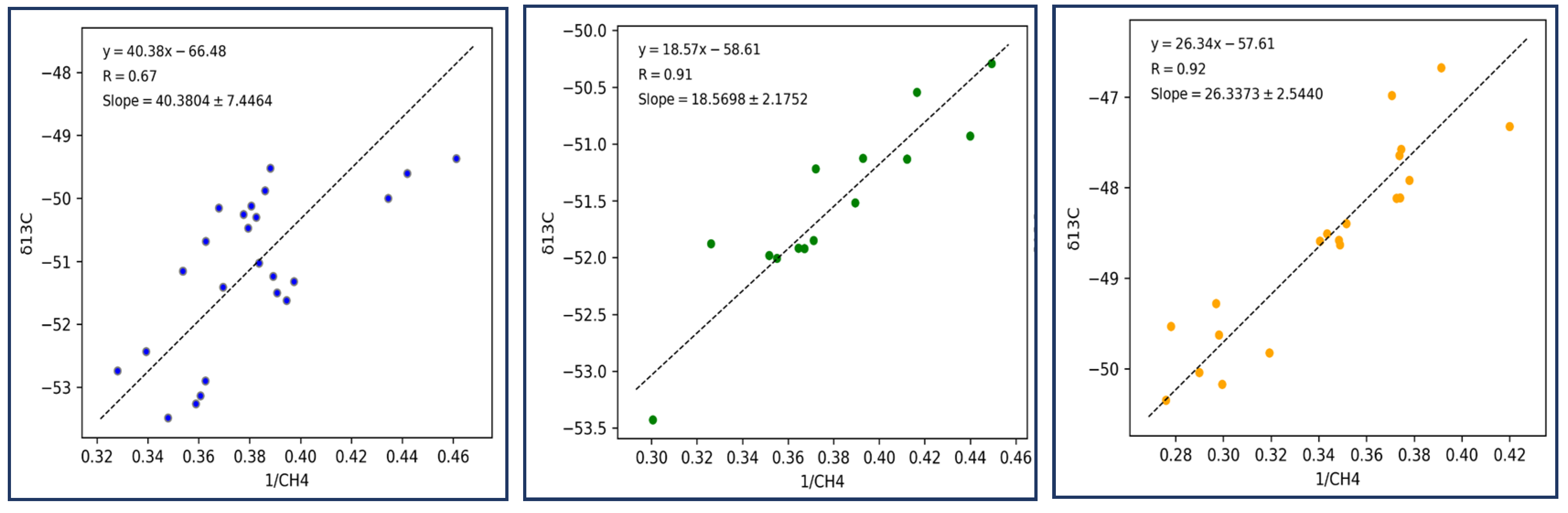
3.4.4. Keeling Plots for the High-Methane Episodes

To study CH₄ sources with the prevailing impact on CH₄ concentration at the IAP RAS site, we used the Keeling plot method [37]. According to this approach, δ¹³C values are plotted against the inverse of the CH₄ mole fractions to calculate the isotopic signature of the methane source responsible for the CH₄ excess over the background. Thus, the intercept of the plot δ¹³CH₄ vs. 1/CH₄ from an atmospheric sample gives the mean isotopic signature of CH₄ sources. Since urban air contains mixed emissions from different sources, it is difficult to obtain convincing Keeling plots and separate CH₄ sources. The exception is the high-methane episodes (CH₄ > 2.2 ppmv), which took place in all seasons of the measurements and lasted from 2 to 6 h (no more than 10% of data).

Keeling plots for the high-methane episodes in 2018–2020 (Figure 15) show very low values of ¹³C: −58.61 ± 0.83‰ and −57.61 ± 0.88‰, for summer and spring–autumn episodes, correspondingly, and −66.48 ± 2.84‰ for winter episodes. Such signatures (Table 1) can characterize an impact of the ¹³C-depleted CH₄ transported from landfills, aeration station, and the Moscow River located in the southeast of the Moscow region (Figure S2). The warm winter of 2020 characterized by positive air temperatures (Figure 2) could lead to snow thawing and activation of CH₄ microbial emissions from urban water ponds and landfills.

Three-hour backward HYSPLIT trajectories for the high-methane episodes confirm air transport from the east–southeast of Moscow (as was also shown from the analysis of CH4 concentration according to the wind direction from the Balchug station (Figure 8)) where microbial CH₄ sources are located (Figure S2).

The obtained results show an important impact of remote CH₄ microbial sources and oil storages on CH₄ concentration in the center of the city, which can help in targeted mitigation efforts.

4. Conclusions

The January 2018–December 2020 measurements of CH₄ mixing ratio and its stable isotope ¹³C along with CO and benzene at the novel IAP RAS site in the center of Moscow city were used to estimate the contributions of various methane emission sources to the observed CH₄ levels under a range of pollutant mixing conditions.

Observations demonstrate stable methane levels throughout the year, ranging from 2.05–2.10 ppmv in winter to 2.02–2.06 ppmv in summer on a monthly basis, with the observed seasonal variation controlled by both the local emissions and long-range transport from upwind sources.

Low δ¹³C values in summer (<−49‰ in more than 50% of observations) provide evidence for a comparatively more significant contribution of microbial CH₄ sources to the observed CH₄ abundance and seasonal variability. In winter, the influence of sources enriched by δ¹³C (natural gas facilities and fossil fuel sources) is found to be more significant compared to the microbial ones, with δ¹³C > −50‰ in about 75% of night- and daytime measurements. The most δ¹³C-depleted CH₄ (up to −56‰) is observed in the anomalously warm and dry summers of 2018 and 2019 as well as in November and December of 2020, marked with warm weather conditions as well, indicating an impact of the methane emissions from microbial sources (municipal drainage, landfills, aeration station, and freshwater reservoirs) on CH₄ concentration at the center of Moscow in these periods.

In the CH₄ diurnal cycle, there is a nighttime increase in methane levels in summer (up to 2.6 ppmv) which is likely attributed to the methane accumulation under the nocturnal inversion layer due to nearby sources and across-city transport from microbial CH₄ sources in the east and southeast parts of Moscow. The latter was most frequently observed in winter months under anticyclonic weather conditions. Diurnal changes in δ¹³C values were found to be insignificant both in summer and in winter, supporting the emission sources affecting the site being independent of any particular time of day.

The regional baseline mixing ratios of CH₄ ([CH₄]_base) and CO ([CO]_base), as well as contribution of urban methane emissions due to vehicle exhausts (∆[CH₄]_auto) and the other sources (mainly microbial activity and gas facility and storage systems) (∆[CH₄]_micro), were estimated from orthogonal regression fits for the daytime CH₄, CO, and benzene data on a seasonal basis. The baseline mixing ratios of CH₄ and CO show a distinct seasonal cycle with a maximum in winter and a minimum in summer as a result of seasonal changes in atmospheric radiation and transport processes. Comparing the derived [CH₄]_base values against published data for the same range of years for the Mace Head (MH) station shows a significant contribution of long-range transport to the baseline CH₄ and CO levels in the region of Moscow. The annual average difference between the [CH₄]_base and the MH values (∆[CH₄]_W) equals 0.044 ppmv, which is comparable to the annual amplitude of the observed methane variability in Moscow itself (0.042 ppmv).

The similar comparison between CO data showed the contribution from upwind continental sources to the Moscow baseline CO levels (∆[CO]_W), equaling 0.018 ppmv in winter and 0.041 ppmv in summer, compared to the annual amplitude in the observed CO mixing ratio of ~0.043 ppmv. In the case of methane, emissions from inland ecosystems are the most probable reason for the derived 20% increase in ∆[CH₄]_W value in summer over that in winter, whereas increased oxidation rates for natural nonmethane hydrocarbons along with emissions of biomass burning seem to be the most important sources of the summertime ∆[CO]_W maximum. We conclude, finally, that continental sources of CH₄ and CO, both anthropogenic and biogenic, contribute appreciably to the observed baseline and urban levels of the above species at the IAP RAS site.

The estimated impact of vehicle exhausts (∆[CH₄]_auto) on the measured CH₄ levels is found to be much lower compared to the other urban sources and more important in winter and spring months due to the seasonally enhanced traffic loading in the Moscow city.

High-methane episodes (>2.2 ppmv) were investigated separately to the main body of data to assess possible contribution of specific emission sources contributing to these events. We found that about 70% of δ¹³C measurements during the high-CH₄ episodes were related to the δ¹³C values < −50‰. Keeling plots of these episodes in different seasons of 2018–2020 show the intercept value of about −58.6 ± 0.8‰ and −57.6 ± 0.9‰ for summer and spring–autumn episodes, correspondingly, and −66.5 ± 2.9‰ for winter. Such isotope signatures are most probably associated with CH₄ transport from the southeast Moscow region where large CH₄ microbial sources (landfills, water treatment plants, and the Moscow River) are located. This transport in the form of spatially coherent plumes can also contribute to the higher ∆[CH₄]_micro+ values in winter and spring compared to other seasons. The anomalously warm weather conditions in some winter, spring, and autumn months of the measurement period are obviously related to the observed enhanced contribution of the microbial methane sources to the measured CH₄ levels at the IAP RAS site.

This study is supposed to provide, for the first time, important insights into the long- and short-term variations of CH₄ levels in Moscow city in connection to the local (urban) emissions and long-range transport from upwind continental sources. The results will contribute to elaboration of a default emission inventory in air quality modeling and help to identify the areas for targeted mitigation efforts.

References

1. Arias, P.A.; Bellouin, N.; Coppola, E.; Jones, R.G.; Krinner, G.; Marotzke, J.; Naik, V.; Palmer, M.D.; Plattner, G.-K.; Rogelj, J.; et al. Technical Summary. In Climate Change 2021: The Physical Science Basis. Contribution of Working Group I to the Sixth Assessment Report of the Intergovernmental Panel on Climate Change; Masson-Delmotte, V., Zhai, P., Pirani, A., Connors, S.L., Péan, C., Berger, S., Caud, N., Chen, Y., Goldfarb, L., Gomis, M.I., et al., Eds.; Cambridge University Press: Cambridge, UK; New York, NY, USA, 2021; pp. 33–144. [Google Scholar]
2. Hopkins, F.M.; Ehleringer, J.R.; Bush, S.E.; Duren, R.M.; Miller, C.E.; Lai, C.-T.; Hsu, Y.-K.; Carranza, V.; Randerson, J.T. Mitigation of methane emissions in cities: How new measurements and partnerships can contribute to emissions reduction strategies. Earth’s Future 2016, 4, 408–425. [Google Scholar] [CrossRef]
3. Marcotullio, P.J.; Sarzynski, A.; Albrecht, J.; Schulz, N.; Garcia, J. The geography of global urban greenhouse gas emissions: An exploratory analysis. Clim. Chang. 2013, 121, 621–634. [Google Scholar] [CrossRef]
4. Zazzeri, G.; Lowry, D.; Fisher, R.E.; France, J.L.; Lanoisellé, M.; Grimmond, C.S.B.; Nisbet, E.G. Evaluating methane inventories by isotopic analysis in the London region. Sci. Rep. 2017, 7, 4854. [Google Scholar] [CrossRef] [PubMed]
5. Townsend-Small, A.; Tyler, S.C.; Pataki, D.E.; Xu, X.; Christensen, L.E. Isotopic measurements of atmospheric methane in Los Angeles, California, USA: Influence of “fugitive” fossil fuel emissions. J. Geophys. Res. 2012, 117, D07308. [Google Scholar] [CrossRef]
6. Gioli, B.; Toscano, P.; Lugato, E.; Matese, A.; Miglietta, F.; Zaldei, A.; Vaccari, F.P. Methane and carbon dioxide fluxes and source partitioning in urban areas: The case study of Florence, Italy. Environ. Pollut. 2012, 164, 125–131. [Google Scholar] [CrossRef] [PubMed]
7. Hsu, Y.K.; VanCuren, T.; Park, S.; Jakober, C.; Herner, J.; FitzGibbon, M.; Blake, D.R.; Parrish, D.D. Methane emissions inventory verification in southern California. Atmos. Environ. 2009, 44, 1–7. [Google Scholar] [CrossRef]
8. Wunch, D.; Wennberg, P.O.; Toon, G.C.; Keppel-Aleks, G.; Yavin, Y.G. Emissions of greenhouse gases from a North American megacity. Geophys. Res. Lett. 2009, 36, 1–5. [Google Scholar] [CrossRef]
9. Brandt, A.R.; Heath, G.A.; Kort, E.A.; O’Sullivan, F.; Pétron, G.; Jordaan, S.M.; Tans, P.; Wilcox, J.; Gopstein, A.M.; Arent, D.; et al. Methane leaks from North American natural gas systems. Science 2014, 343, 733–735. [Google Scholar] [CrossRef]
10. Sriskantharajah, S.; Fisher, R.E.; Lowry, D.; Aalto, T.; Hatakka, J.; Aurela, M.; Laurila, T.; Lohila, A.; Kuitunen, E.; Nisbet, E.G. Stable carbon isotope signatures of methane from a Finnish subarctic wetland. Tellus Ser. B 2020, 64, 18818. [Google Scholar] [CrossRef]
11. Bakkaloglu, S.; Lowry, D.; Fisher, R.E.; Menoud, M.; Lanoisellé, M.; Chen Thomas Rockmann, T.; Nisbet, E.G. A Stable isotopic signatures of methane from waste sources through atmospheric measurements. Atmos. Environ. 2022, 276, 119021. [Google Scholar] [CrossRef]
12. Elansky, N.F.; Shilkin, A.V.; Ponomarev, N.A.; Zakharova, P.V.; Kachko, M.D.; Poliakov, T.I. Spatiotemporal Variations in the Content of Pollutants in the Moscow Air Basin and Their Emissions. Izv. Atmos. Ocean. Phys. 2022, 58, 80–94. [Google Scholar] [CrossRef]
13. Fisher, R.; Lowry, D.; Wilkin, O.; Sriskantharajah, S.; Nisbet, E.G. High-precision, automated stable isotope analysis of atmospheric methane and carbon dioxide using continuous flow isotope-ratio mass spectrometry. Rapid Commun. Mass Spectrom. 2006, 20, 200–208. [Google Scholar] [CrossRef] [PubMed]
14. Levin, I.; Glatzel-Mattheier, H.; Marik, T.; Cuntz, M.; Schmidt, M.; Worthy, D.E.J. Verification of German methane emission inventories and their recent changes based on atmospheric observations. J. Geophys. Res. 1999, 104, 3447–3456. [Google Scholar] [CrossRef]
15. Lopez, M.; Sherwood, O.A.; Dlugokencky, E.J.; Kessler, R.; Giroux, L.; Worthy, D.E.J. Isotopic signatures of anthropogenic CH4 sources in Alberta, Canada. Atmos. Environ. 2017, 164, 280–288. [Google Scholar] [CrossRef]
16. Stevens, C.; Engelkemeir, A. Stable Carbon Composition of Methane from Some Natural and Anthropogenic Sources. J. Geophys. Res. 1989, 93, 725–733. [Google Scholar] [CrossRef]
17. Varga, T.; Fisher, R.E.; France, J.L.; Haszpra, L.; Jull, A.J.T.; Lowry, D.; Major, I.; Molnár, M.; Nisbet, E.G.; László, E. Identification of potential methane source regions in Europe using δ13CCH4 measurements and trajectory modeling. J. Geophys. Res. Atmos. 2021, 126, e2020JD033963. [Google Scholar] [CrossRef]
18. Xueref-Remy, I.; Zazzeri, G.; Br’eon, F.M.; Vogel, F.; Ciais, P.; Lowry, D.; Nisbet, E.G. Anthropogenic methane plume detection from point sources in the Paris megacity area and characterization of their δ13C signature. Atmos. Environ. 2020, 222, 117055. [Google Scholar] [CrossRef]
19. Elansky, N.F. Air quality and CO emissions in the Moscow megacity. Urban Clim. 2014, 8, 42–56. [Google Scholar] [CrossRef]
20. Elansky, N.F.; Shilkin, A.V.; Ponomarev, N.A.; Semutnikova, E.G.; Zakharova, P.V. Weekly patterns and weekend effects of air pollution in the Moscow megacity. Atmos. Environ. 2020, 224, 117303. [Google Scholar] [CrossRef]
21. Berezina, E.; Moiseenko, K.; Vasileva, A.; Pankratova, N.; Skorokhod, A.; Belikov, I.; Belousov, V. Emission Ratios and Source Identification of VOCs in Moscow in 2019–2020. Atmosphere 2022, 13, 257. [Google Scholar] [CrossRef]
22. Berezina, E.; Moiseenko, K.; Skorokhod, A.; Pankratova, N.V.; Belikov, I.; Belousov, V.; Elansky, N.F. Impact of VOCs and NOx on Ozone Formation in Moscow. Atmosphere 2020, 11, 1262. [Google Scholar] [CrossRef]
23. PICARRO. G2132-iδ13C High Precision Isotopic CH4 CRDS Analyzer. Available online: https://www.picarro.com/support/library/documents/g2132i_analyzer_datasheet (accessed on 27 February 2023).
24. Pankratova, N.; Skorokhod, A.; Belikov, I.; Belousov, V.; Muravya, V.; Flint, M. Ship-Borne Observations of Atmospheric CH4 and δ13C Isotope Signature in Methane over Arctic Seas in Summer and Autumn 2021. Atmosphere 2022, 13, 458. [Google Scholar] [CrossRef]
25. Pankratova, N.; Skorokhod, A.; Belikov, I.; Elansky, N.; Rakitin, V.; Shtabkin, Y.; Berezina, E. Evidence of atmospheric response to methane emissions from the east siberian arctic shelf. Geogr. Environ. Sustain. 2018, 11, 85–92. [Google Scholar] [CrossRef]
26. Dlugokencky, E.J.; Myers, R.C.; Lang, P.M.; Masarie, K.A.; Crotwell, A.M.; Thoning, K.W.; Hall, B.D.; Elkins, J.W.; Steele, L.P. Conversion of NOAA atmospheric dry air CH4 mole fractions to a gravimetrically prepared standard scale. J. Geophys. Res. 2005, 110, D18306. [Google Scholar] [CrossRef]
27. Thompson, A.; Rudolph, J.; Rohrer, F.; Stein, O. Concentration and stable carbon isotopic composition of ethane and benzene using a global three-dimensional isotope inclusive chemical tracer model. J. Geophys. Res. 2003, 108, 4373. [Google Scholar] [CrossRef]
28. Halliday, H.S.; Thompson, A.M.; Wisthaler, A.; Blake, D.R.; Hornbrook, R.S.; Mikoviny, T.; Müller, M.; Eichler, P.; Apel, E.C.; Hills, A.J. Atmospheric benzene observations from oil and gas production in the Denver-Julesburg Basin in July and August 2014. J. Geophys. Res. Atmos. 2016, 121, 11055–11074. [Google Scholar] [CrossRef]
29. Holloway, T.; Levy, H.; Kasibhatla, P. Global distribution of carbon monoxide. J. Geophys. Res. 2000, 105, 12123–12147. [Google Scholar] [CrossRef]
30. Elansky, N.F. (Ed.) Atmospheric Composition Observations Over Northern Eurasia Using the Mobile Laboratory: TROICA Experiments; International Science and Technology Center: Astana, Kazakhstan, 2009; p. 84. [Google Scholar]
31. Lan, X.; Dlugokencky, E.J.; Mund, J.W.; Crotwell, A.M.; Crotwell, M.J.; Moglia, E.; Madronich, M.; Neff, D.; Thoning, K.W. Atmospheric Methane Dry Air Mole Fractions from the NOAA GML Carbon Cycle Cooperative Global Air Sampling Network, 1983–2021, Version: 2022-11-21. 2022. Available online: https://gml.noaa.gov/ccgg/trends_ch4/ (accessed on 27 February 2023).
32. Naus, S.; Röckmann, T.; Popa, M.E. The isotopic composition of CO in vehicle exhaust. Atmos. Environ. 2018, 177, 132–142. [Google Scholar] [CrossRef]
33. Brandt, S. Statistical and Computational Methods in Data. Analysis; Springer: New York, NY, USA, 1998. [Google Scholar]
34. Wong, K.W.; Fu, D.; Pongetti, T.J.; Newman, S.; Kort, E.A.; Duren, R.; Hsu, Y.-K.; Miller, C.E.; Yung, Y.L.; Sander, S.P. Mapping CH4: CO2 ratios in Los Angeles with CLARS-FTS from Mount Wilson, California. Atmos. Chem. Phys. 2015, 15, 241–252. [Google Scholar] [CrossRef]
35. Janssens-Maenhout, G.; Crippa, M.; Guizzardi, D.; Muntean, M.; Schaaf, E.; Dentener, F.; Bergamaschi, P.; Pagliari, V.; Olivier, J.G.J.; Peters, J.A.H.W.; et al. EDGAR v4.3.2 Global Atlas of the three major greenhouse gas emissions for the period 1970–2012. Earth Syst. Sci. Data 2019, 11, 959–1002. [Google Scholar] [CrossRef]
36. Bloom, A.A.; Bowman, K.W.; Lee, M.; Turner, A.J.; Schroeder, R.; Worden, J.R.; Weidner, R.; McDonald, K.C.; Jacob, D.J. A global wetland methane emissions and uncertainty dataset for atmospheric chemical transport models (WetCHARTs version 1.0). Geosci. Model Dev. 2017, 10, 2141–2156. [Google Scholar] [CrossRef]
37. Keeling, C.D. The concentration and isotopic abundances of atmospheric carbon dioxide in rural areas. Geochim. Cosmochim. Acta 1958, 13, 322–334. [Google Scholar] [CrossRef]
Figure 1. Spatial locations of IAP RAS (red crisscross) site, MEM sites (blue rectangles: MSU, CHE, KOZ, GUR), and the Balchug weather station (blue rectangle: BAL).
Atmosphere 14 00830 g001
Figure 2. Average, minimum, and maximum daily average temperatures for each month of the observed period.
Atmosphere 14 00830 g002
Figure 3. Windspeed (m/s) diagrams for winter (a) and summer (b) of 2018–2020.
Atmosphere 14 00830 g003aAtmosphere 14 00830 g003b
Figure 4. Monthly statistics of daytime (10:00–17:00 local time) hourly mean (a,c,e) CH4 and (b,d,f) δ13C values observed in the years (a,b) 2018, (c,d) 2019, and (e,f) 2020 at the IAP RAS site (cross—median, open square—mean, bars—10th–90th percentile range) and at the MEM network (black line—medians, shaded area—10th–90th percentile range of hourly mean values across the following stations with best correlation (R > 0.5) with the IAP RAS measurements: Kozhuhovo, Guriyanova, MSU, and Cheremushki).
Atmosphere 14 00830 g004
Figure 5. Monthly statistics of daytime (10:00–17:00 local time) hourly mean (a) CH4 and (b) δ13C values observed in years 2018–2020 at the IAP RAS site (cross—median, square—mean, bars—10th–90th percentile range) and at the MEM network (black line—medians, shaded area—10th–90th percentile range of hourly mean values across the following stations with best correlation (R > 0.5) with the IAP RAS measurements: Kozhuhovo, Guriyanova, MSU, and Cheremushki).
Atmosphere 14 00830 g005
Figure 6. Hourly mean (a) CH4 (ppmv) and (b) δ13C (‰) values observed in summer (a) and winter (b) months of 2018–2020 at the IAP RAS site (cross—median, square—mean, vertical dotted line—the 10th–90th percentile range).
Atmosphere 14 00830 g006
Figure 7. Hourly deviations of CH4 from its daily averages in winter of (a) 2018 (east wind is prevailing), (b) 2019 (east and west winds are prevailing), and (c) 2020 (west wind is prevailing) at the IAP RAS site (cross—median, square—mean, bars—10th–90th percentile range) and at the MEM network (black line—medians, shaded area—10th–90th percentile range across the following stations with best correlation (R > 0.5) with the IAP RAS measurements: Kozhuhovo, Guriyanova, MSU, and Cheremushki).
Atmosphere 14 00830 g007aAtmosphere 14 00830 g007b
Figure 8. CH4 concentration according to the wind direction (in degrees; the North is set at 0°) from the Balchug station (3 h data) in summer and winter of 2018–2020. Bar lengths (in %)—frequency of CH4 concentration records.
Atmosphere 14 00830 g008
Figure 9. δ13C according to the wind direction (in degrees; the North is set at 0°) from the Balchug station (3 h data) in summer and winter of 2018–2020. Bar lengths (in %)—frequency of CH4 concentration records.
Atmosphere 14 00830 g009
Figure 10. Box plots of 3 h average CH4 according to the wind direction sectors (1: 0–90°; 2: 90–180°; 3: 180–270°; 4: 270–360°; 0 is north) in (a) warm (May–September) and (b) cold (October–April) periods of the years 2018–2020. The shaded box is the interquartile range (25–75%). The horizontal line inside the box is the median and the square is the mean value. The whiskers are minimum and maximum values.
Atmosphere 14 00830 g010
Figure 11. Frequency distribution of δ13C in different seasons and times of the day in 2018–2020.
Atmosphere 14 00830 g011
Figure 12. Orthogonal regression fits of 1 h data in summer (a) and in winter (b) of 2018–2020. Red circles are high-methane episodes (CH4 > 2.2 ppmv).
Atmosphere 14 00830 g012
Figure 13. Frequency distribution of δ13C during the high-CH4 episodes in 2018–2019.
Atmosphere 14 00830 g013
Figure 14. Orthogonal regression fits of 1 h daytime (10 a.m.–19 p.m.) CH4 data in winter (a), spring (b), summer (c), and autumn (d) of 2018–2020. High-CH4 episodes (CH4 > 2.2 ppmv) are excluded. The solid line is the best fit via orthogonal linear regression. Linear fit equation and R values are shown for all panels.
Atmosphere 14 00830 g014
Figure 15. Keeling plots for high-methane episodes (>2.2 ppmv): winter (blue points), summer (green points), and spring–autumn (orange points) of 2018–2020.
Atmosphere 14 00830 g015