Abstract
Southeast Europe is considered one of the most vulnerable regions in the context of climate change, and projected future summer warming is expected to exceed global rates significantly. Despite the importance of this problem, there have been few studies that utilized Coupled Model Intercomparison Project Phase 5 (CMIP5) Global Circulation Models (GCMs) and the multi-model ensemble approach to examine extreme heat events on a regional scale. Additionally, the NEX-GDDP dataset, successfully applied in other parts of the world to assess extreme heat, has not yet been utilized for Southeast Europe. This study aims to fill that gap, presenting the time evolution and spatial distribution of extreme heat events in Southeast Europe for the historical period 1950–2005 and for the expected future climate up to the end of the 21st century based on the NEX-GDDP dataset. In order to leverage the strengths of the multi-model ensemble approach, a set of purpose-tailored indicators, such as the annual number of hot days, the maximum number of consecutive hot days, and hot spell duration at different thresholds, is computed by the daily maximum temperature data from all datasets, produced by NEX-GDDP (21 for the historical period and 42 for the future period). The E-OBS dataset is used as a reference for evaluating the NEX-GDDP’s capability to simulate the features of the observed historical extreme heat events. The results show that the multi-model ensemble can satisfactorily capture the occurrence of extreme heat events in the historical period, and therefore it is reasonable to assume that the NEX-GDDP dataset has the potential to reproduce such extremes in the projected future. The study provides clear evidence that the persistence and spatial extent of extreme heat will increase significantly. Some indicators that were not relevant for the historical period due to the high-temperature threshold will become helpful in assessing extreme heat in Southeast Europe in the latter part of the century. Thus, under the RCP8.5 scenario, the area-averaged duration of hot spells at 32 °C and 34 °C will increase from near zero in 1976–2005 to 60 and 45 days, respectively, by the end of the century. The indicators used in the study may be helpful for decision-makers to implement climate change mitigation strategies and actions adequately. The findings are consistent with general tendencies in maximum temperatures considered in our previous works but also with the outcomes of recent studies dedicated to the future climate of the region.
1. Introduction
Surface air temperature extremes affect the natural ecosystems and biodiversity [1,2], agriculture [3,4], water resources [5], and the various sectors of the world economy [6,7], as well as the human health and well-being, especially of the vulnerable part of the population [8,9]. Under the changing climate, both warm spells and heat waves with increasing frequency, intensity, and duration are reported worldwide [10,11]. The major part of Europe has experienced its most severe heat wave in recent two decades: 2003 in Western Europe, 2010 in Eastern Europe, 2018 in Scandinavia, and 2021 in the Mediterranean, with record-breaking temperatures [12,13,14,15,16,17,18,19]. Extreme heat events (EHEs) trends and projections exhibit increasing frequency and intensity, implying elevated risk and the need for elaboration of improved mitigation strategies. As a result, the number of scientific papers on heat waves and their impacts has steadily risen.
In the eastern Mediterranean region, which includes Southeast Europe (SEE), a general warming trend prevails, most pronounced since the 1980s [20,21,22,23]. Summer temperatures significantly contribute to this trend, associated with both an increase in long-term averages and an increase in the number of extreme heat events [24,25,26,27]. Although hot weather periods are a typical summertime phenomenon in Southern Europe, severe heatwaves, which relatively rarely occurred even in the late 20th century, may become the norm by the middle or end of the century [28,29]. Overall, the region is proving to be a ’hotspot’ of climate change [30,31,32] and projected future summer warming is expected to exceed global rates by 40% [33].
GCMs are the primary source of information for understanding and evaluating Earth’s climate variability and change in the past, present and future [34,35,36]. Many studies have attempted to project the future changes of extremely high temperatures over different regions using single GCM [37], multiple GCMs and model ensembles (e.g., [6,38]), and GCM-driven regional climate models (RCMs) [39], applying various indicators of extreme heat. Regardless of the differences in the utilized methodology and considered domain, they reveal increased duration, spatial extent, and severity of heat waves in the generally warmer future climate.
In the last decades, many researchers have favored a multi-model ensemble (MME) approach in which simulations of future conditions are produced with multiple climate models (or model versions) rather than just one [40]. This concept is widely used as it reduces the random errors associated with the models and suppresses internal variability [41]. Despite the existing criticism and the ongoing debate about the construction possibilities of MMEs, the common opinion is that they are an indispensable tool for future climate projection and the quantification of its uncertainty [42,43].
The main objective of this study is to quantify projected changes and trends of EHEs in SEE under the Representative Concentration Pathway (RCP) scenarios RCP4.5 and RCP8.5. We have utilized the U.S. National Aeronautics and Space Administration (NASA) Earth Exchange Global Daily Downscaled Projections (NEX-GDDP) dataset for the period 1950–2100 to calculate a set of EHEs-indicators and evaluate the changes in EHEs features from the last 30 years in the baseline period to the latter 30 years in the 21st century by applying the MME approach. The NEX-GDDP dataset has been successfully utilized for the quantification of projected changes of EHEs, for example, over Pakistan [44], China [45], and three mega-regions (the Eastern United States, Europe, and Eastern Asia) [46]. Regardless of the significant vulnerability of SEE to extreme heat, there are relatively few studies based on CMIP5 GCMs, especially using multi-model ensembles. To our knowledge, the NEX-GDDP dataset has not been employed in regional studies of EHEs. However, a recent study by Chervenkov and Slavov [47] provides general evidence of the NEX-GDDP MME’s skill in reproducing historical climate, which motivated us to explore its capability to reproduce EHEs. Therefore, the novelties of this work include: (i) using the perspective NEX-GDDP dataset to quantify projected changes of EHEs in SEE, (ii) explicitly considering the MME approach using the complete set of NEX-GDDP GCMs, and (iii) utilizing EHE-indicators, whose suitability for regional assessments in the present climate has already been evaluated in our previous works [48,49]. Overall, this study can be seen as a natural continuation of [47] and [48].
2. Material and Methods
2.1. Study Area
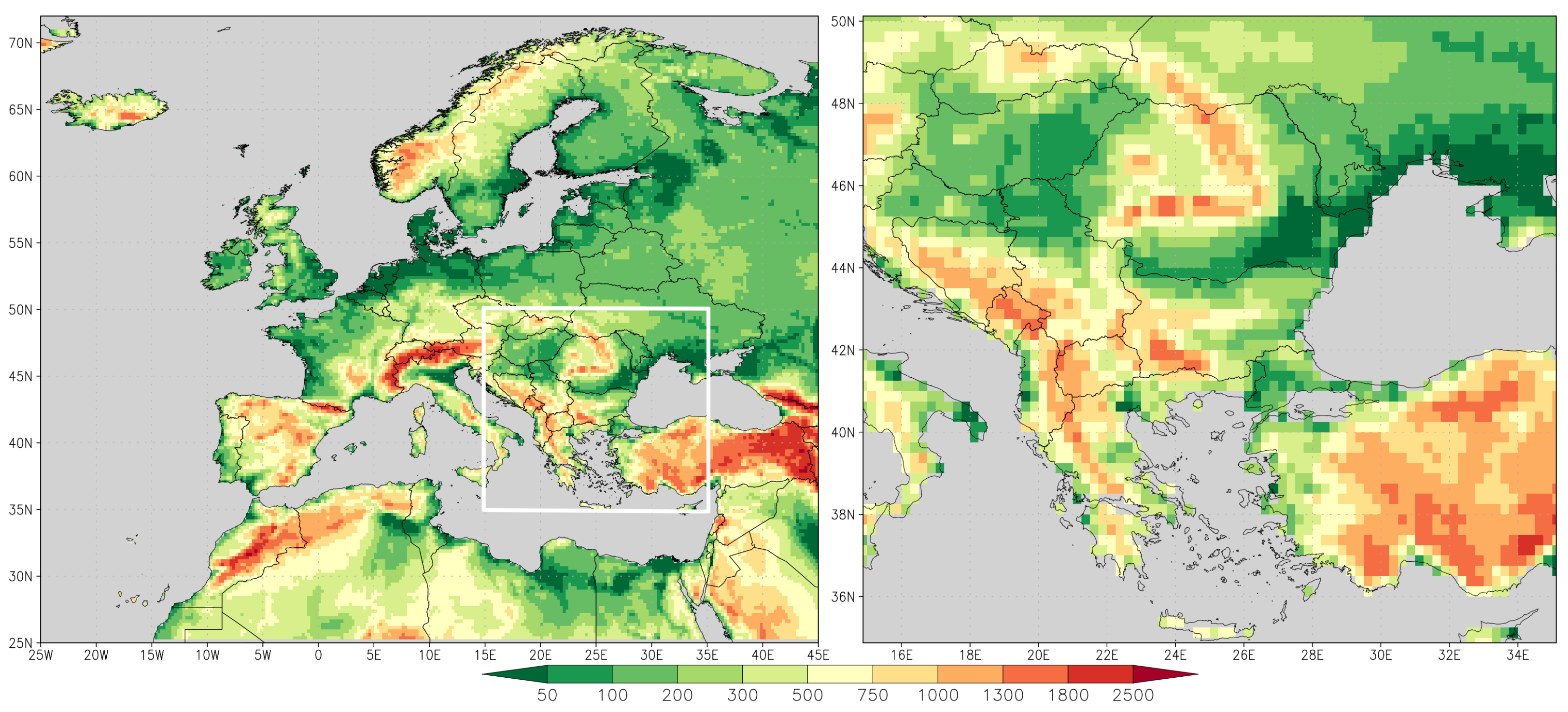
The study area is the same as in [47]—with geographical boundaries of 35° N–50° N and 15° E–35° E. The elevation data from the daily gridded dataset E-OBS at 0.25° resolution is used to present the topography of the domain (Figure 1).
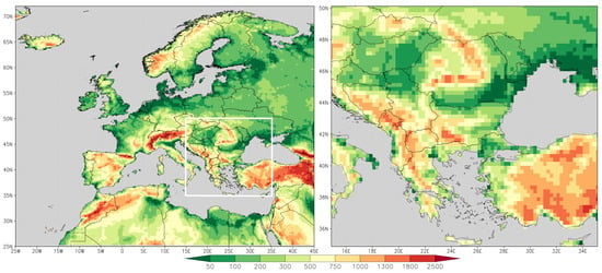
Figure 1.
Elevation above sea level (unit: m) of the considered domain (on right) as part of the E-OBS domain (on left).
Although the domain is relatively small, it features rather complex topography, comprising deep valleys, high mountains (up to 3000 m a.s.l), and a long, fragmented coastline. This domain falls almost entirely into the Mediterranean region, defined by the Mediterranean Experts on Climate and Environmental Change [33]. According to the updated Köppen-Geiger classification [50], several climate subtypes can be distinguished, including Mediterranean climates with a dry hot/warm summer (Csa/Csb), temperate climates with no dry hot/warm summer (Cfa/Cfb), semiarid mid-latitude climates (BSk) and humid or dry continental climates with hot/warm summer (Dfa/Dfb or Dsa/Dsb, respectively) [51].
2.2. Data
Similarly to other NEX-GDDP-based studies of extreme heat [44,45,46], the calculation of the EHEs-indicators used in this study requires only data for the daily maximum temperature (hereafter: tx). To identify the observed historical EHEs features, the tx, with a horizontal resolution of 0.25° spanning 1950–2005, was retrieved from E-OBS v23.1e of the European Climate Assessment and Dataset (ECA&D) project [52]. E-OBS is a de facto standard reference for evaluating the RCMs participating in the Coordinated Downscaling Experiment - European Domain (EURO-CORDEX) [53]; it is also used frequently for various other applications, including monitoring of climate extremes. Alongside the improved uncertainty quantification, the E-OBS ensemble versions generally present temperature extremes better than their predecessors. In the present study, E-OBS is used as reference for the historical period.
The tx needed for quantification of the projected changes of EHEs are obtained from the NEX-GDDP dataset [54]. It compiles 42 downscaled climate projections from 21 GCMs runs conducted under CMIP5 [34] and across two (RCP4.5 and RCP 8.5) of the four radiative forcing scenarios known as RCPs [55]. The labels for the RCPs provide a rough estimate of the radiative forcing in the year 2100 (relative to pre-industrial conditions) [34]. The RCP4.5 is a scenario that stabilizes radiative forcing at at 4.5 W·m−2 in the year 2100 without ever exceeding that value [56]. The RCP8.5 scenario suggests a rising pathway with 8.5 W·m−2 in 2100 [57]. Among others, these scenarios are most commonly regarded as ‘realistic’ (RCP4.5) and ‘pessimistic’ (RCP8.5) and are widely utilized in the expert community. The purpose of the NEX-GDDP is to provide a global, high-resolution (0.25°× 0.25° or approximately 25 km × 25 km in the mid-latitudes), bias-corrected climate change projections for the period 2006–2100, as well as a historical experiment for each model for the baseline period 1950–2005. The used Bias-Correction Spatial Disaggregation method is a statistical downscaling algorithm specifically developed to address the basic limitations of global GCM outputs—the relatively coarse spatial resolution and the systematic bias in their statistical characteristics concerning the ground observations [58].
The primary goal of the NEX-GDDP developers and distributors is to assist the science community in conducting studies of climate change impacts at local to regional scales. Subsequently, it is used for many applications around the globe as an assessment of the Indian summer monsoon [41,59,60] and as general investigations on near- and long-term climate projections over China [61] and Southeast Asia [35]. The overall conclusion is that the NEX-GDDP product offers considerable improvements over CMIP5 GCM hindcasts and projections at regional-to-local scales, with an unchanged global long-term increment [61].
2.3. Methodology
Although the risks posed by extreme heat are far-reaching, the metrics and thresholds used to define extremes and quantify their impacts vary within and across sectors [1,38,62]. Moreover, the definitions of hot days and EHEs differ significantly even across the NEX-GDDP-based studies [45]. Thus, in work [45], the simple thresholding method is used, adopting three temperature levels of the daily maximum temperature. The study [44] is based on the Heat Wave Duration Index (HWDI), defined as a period of at least 6 consecutive days when tx exceeds the mean maximum temperature by 5 °C. In [46], a day with a maximum temperature exceeding the 90th percentile centered on a 5-day window for the base period is counted as one extreme heat day. In the present study, we apply extremely hot weather indicators validated for the climate conditions of Bulgaria [49] and, more recently, for SEE [48]. Our methodology is based on three climate indicators defined as follows:
- 1.
- Annual number of hot days (nhd), i.e., the annual count of days when °C;
- 2.
- Maximum number of consecutive hot days (chd), i.e., the longest continuous calendar period in the year when °C;
- 3.
- Hot spells duration at different thresholds (hsd32/34/36/38/40), i.e., the annual count of days when , 34, 36, 38 and 40 °C for at least 6, 5, 4, 3 and 2 consecutive days, respectively.
These indicators allow us to assess the changes in the severity of extreme heat in light of the worsening of daytime thermal conditions, the increase in prolonged hot weather, and the frequency of EHEs. The good agreement of the proposed hsd indicator with the widely used Excess Heat Factor index [63] is the main proof of its suitability for regional studies of extreme heat. The methodology of determining the threshold values as 2, 5, 10, 20 and 50-year return levels for tx and 90th percentile for hot spells duration follows the concept and terminology of WMO and IPCC [32,64].
The NEX-GDDP data for all 21 GCMs (see in Appendix A the list of the GCMs) for the historical experiment and both future projections were used in the previous study [47]. Working with the complete set of 21 GCMs is a analogous to [41,45,61] and rather different approach than the one applied in [60], where only five models are used. The set of the considered EHEs-indicators is computed from the output tx for each model individually and from the tx extracted from E-OBS, which is used as a reference. All computations are performed on a yearly basis. Next, the MMEs median (MX50), 25th and 75th percentile (lower and upper quartile, noted further MX25 and MX75) are computed for the historical period 1950–2005 and the projected future climate in 2006–2100. Both quartiles and the difference MX75-MX25 are the most commonly used MME parameters in climatological studies (see, for example, [36]). The multiyear mean values for the 30-year time slices 1976–2005 and 2071–2100 are calculated by simple time averaging. The processing of netCDF files is performed through the authors’ purpose-built Linux bash shell scripts using the powerful tool Climate Data Operator [65]. The use of MME statistical features for analyzing the considered extreme heat indicators is generally similar to the approach in [44], where the median of HWDI is utilized. Among the NEX-GDDP-based research, one of the novelties in our study is the explicit consideration of the spatial distributions of the MME MX25 and MX75.
3. Results and Discussion
3.1. Present Climate Evaluation
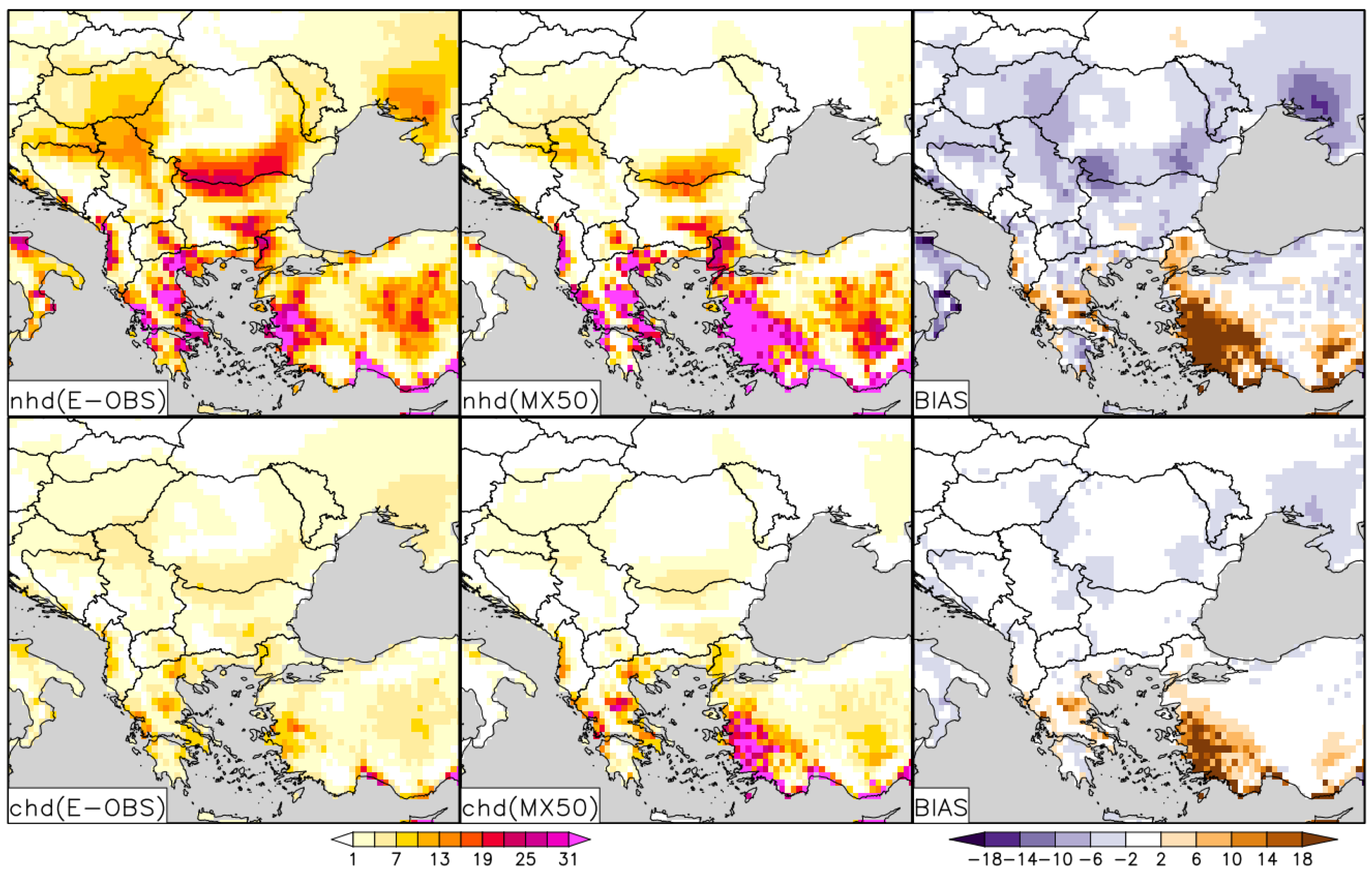
The ability of the NEX-GDDP ensemble to reproduce the spatial and temporal variability of EHEs in the historical period (1950–2005) has been evaluated at multiyear and annual time scales. The comparison between the multiyear mean values of NEX-GDDP MME MX50 and E-OBS, referred to as ‘model’ and ‘reference’ for the considered indicators, respectively, is presented in in Figure 2 and Figure 3.
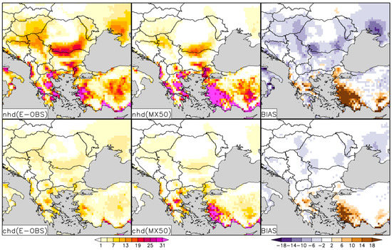
Figure 2.
Comparison of multiyear mean values (1950–2005) of NEX-GDDP MME MX50 and E-OBS for nhd and chd, as well as the absolute bias (model-reference). The units are days.
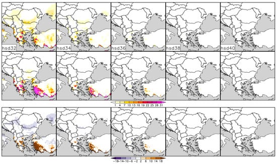
Figure 3.
Comparison of multiyear mean values (1950–2005) of E-OBS (first row) and NEX-GDDP MME MX50 (second row) for hsd32/34/36/38/40, as well as the absolute bias (model-reference) in the third row. The units are days.
It is evident that there are certain similarities between the spatial patterns of EHEs-indicators derived from NEX-GDDP MME and E-OBS. However, several discrepancies exist in reproducing the magnitude of indicators, such as an underestimation of nhd and chd over the southern parts of Ukraine and Romania. On the other hand, the location and spatial extent of the main maximums over Turkey and Greece are well-reproduced, although overestimated. In general, NEX-GDDP MME MX50 tends to overestimate the maximums, particularly over Türkiye, and underestimate the lower values, which are typical for most of the domain. The latter fact could be partially caused by the embedded in the E-OBS processing chain spatial correlation procedure [52], leading to the relatively smoothed tx-field. The biggest bias is registered over the southeastern part of the domain and is more than 14 days for nhd, chd, and hsd32/34. Despite the NEX-GDDP MME disadvantage, this disagreement could be explained to a certain extent by the local weakness of E-OBS caused by the lack of shared with the ECA&D observations [53].
The multiyear means of hsd36/38/40 for the period 1950–2005 are nearly zero practically over the whole domain. These EHEs are relatively rare under historical climate conditions, with long return periods, and their multiyear means are not suitable for long-term analysis for this time-frame.
Researchers use various metrics to evaluate the GCM or RCM simulations. A similar concept is also applied in evaluating the NEX-GDDP data set [35,41,46,47]. However, there is still a debate about selecting and combining performance metrics. In the considered case, the implementation of some well-known metrics is hampered by the fact that they are not defined if the reference and/or model time series consist of zeros. For example, the correlation coefficient (corr) is not defined when the reference/model time series is constant zero, which is the case over the prevailing part of the domain for the hsd indicator at higher tx-thresholds (see Figure 2). Nevertheless, we selected suitable metrics to evaluate the NEX-GDDP MME MX50, namely the root mean square error (RMSE) and the index of agreement (IA) [66]. These statistics are applied in several studies evaluating and utilizing the NEX-GDDP dataset [41,59,60,67]. The IA is defined as follows:
where M and R denote modelled and reference values of the considered indicators indexed by i, N is the time series length, and M and R with overbars are the time series averages. The dimensionless IA reflects the degree to which the modelled variable differs from the reference, and its range is similar to that of , i.e., between 0 (full disagreement) and 1 (perfect fit). Although the IA index is widely used in studies to check the accuracy of a model [68,69], in [66] is argued that the replacement of the quadratic function with linear in Equation (1) results in a more rigorous index:
An additional advantage of IA and the modified version IAm is that both statistical measures are not defined only if all terms in the time series of the reference and model dataset are constant zero (these regions are shown in dark grey in Figure 4).
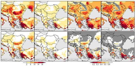
Figure 4.
RMSE (unit: days) and IAm for the nhd, chd, hsd32, and hsd34 according to the subplot titles. The regions where the IAm is not definite are shown in dark grey.
Figure 4 shows the RMSE and IAm for the nhd, chd, hsd32, and hsd34.
Regarding RMSE values, nhd distinguishes with the largest spatial heterogeneity, with a mean value below 10 days. The RMSE fields for the other indicators are more homogeneous, with a mean value around or below 6 days. The spatial patterns of IAm for nhd and chd are similar, with prevailing values in the range of 0.3–0.5. The IAm values for hsd32 and hsd34, where they are defined, ranged from below 0.2 (over southwestern Türkiye) to above 0.6, mainly in the northern part of the domain.
In [61] is emphasized that the ability of NEX-GDDP to capture temperature extremes can be primarily attributed to its high resolution. The presented in this subsection results and those in [47] generally agree with this statement. In fact, grid averaged temperature over-smooths the local sub-grid maximum and/or minimum, and a coarser horizontal resolution (as from the primary GCMs output) results in a larger bias.
3.2. Future Projections of EHEs
We expect the high-resolution NEX-GDDP dataset, which reproduces the historical climatology, to also deliver a more accurate projection of SEE’s future climate than the primary CMIP5 GCMs output [61].
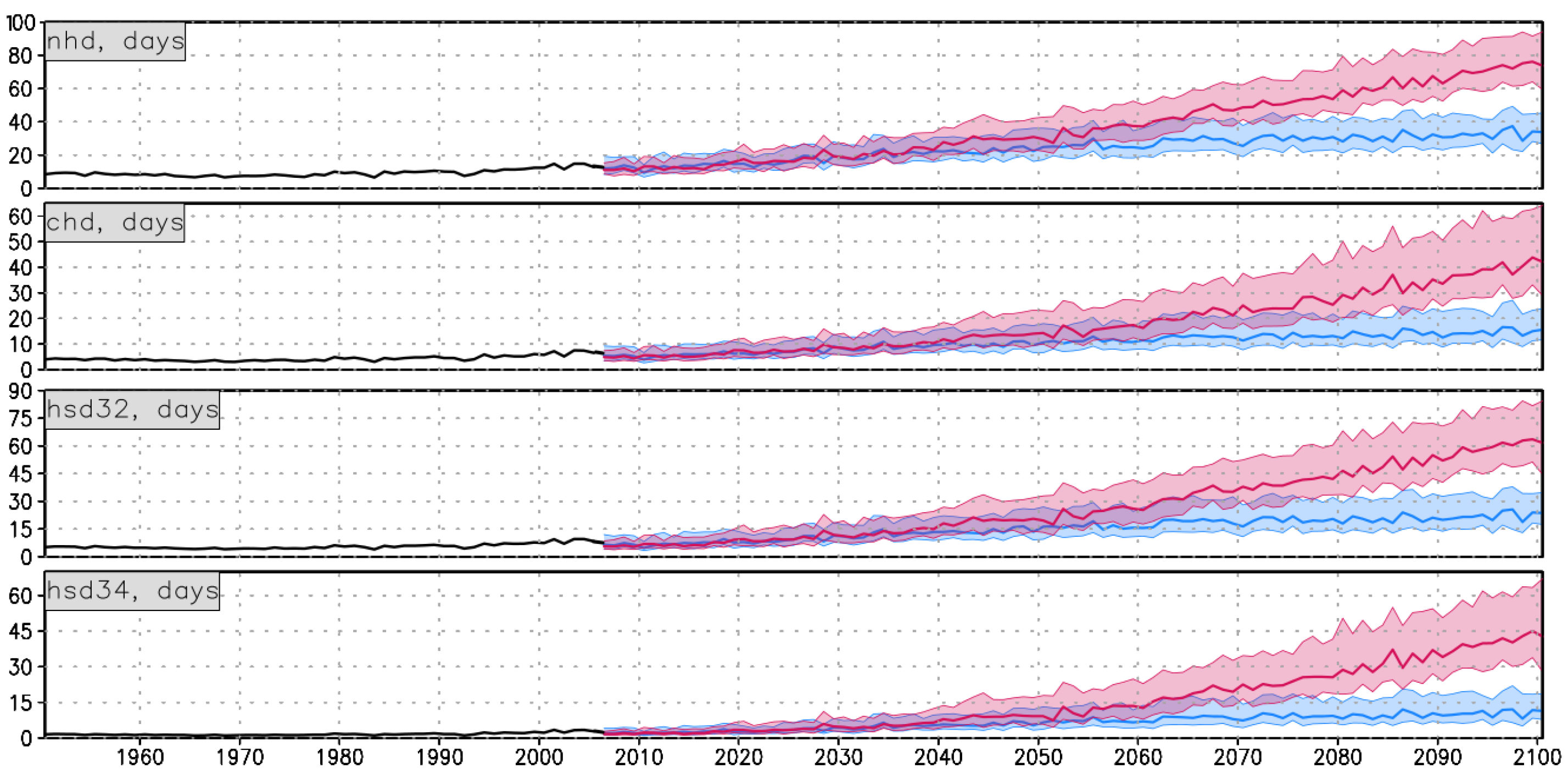
Figure 5, which shows the time series of the areal-averaged (AA) over the whole domain values of EHEs-indicators nhd, chd, hsd32, and hsd34, provides an overall picture of their evolution during the reference period and projected future.
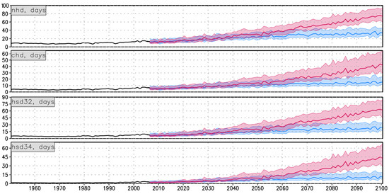
Figure 5.
Time evolution of the AAs of the EHEs-indicators for the reference period (solid black line), for RCP4.5 (in blue), and RCP8.5 (in red) scenario. Solid lines indicate the ensemble median and the shading indicates the ensemble spread.
The most notable result from the analysis of Figure 5 is the steady increase of values of the considered EHEs-indicators for the longer part of the period 1950–2100. A short-term decrease with a relatively small magnitude only is observed in the late fifties and seventies of the 20th century. The increase rate is clearly notable in the historical period after 1980 and especially after the middle of the current century. The work [70] provides clear evidence for the steady increase of some temperature-based indices from the recognized collection of the Expert Team on Climate Change Detection and Indices (ETCCDI) [71] in the interior of SEE during 1950–2016. In our recent study [72], the key ETCCDI climate indices absolute annual maximum of the daily minimum and maximum temperature (TNx and TXx) as well as the warm spell duration index (WSDI) are analyzed for the projected future climate over SEE up to the end of the century. The indices are computed from the bias-corrected output of five CMIP5 global models, forced with all four RCP emission scenarios. The MME MX50 of all indices indicates considerable warming. Thus, The AA of the WSDI during the whole reference period 1981–2010 remains with practically negligible values almost constant. In contrast, the dynamics in the projected future demonstrates steady increase, especially for RCP8.5. Consequently, the MME MX50 for this scenario is over 150 days around the 2080’s. The decade-long tendency of the EHEs-indicators, although based on other methodology, are in principle agreement with the overall outcomes from these studies and are consistent with the general variability of the maximum temperature. The analysis of Figure 5 also shows that the interquartile model spreads in both RCPs practically remain overlapping until the middle of the 21st century. Generally, however, the increase is proportional to the radiative forcing, i.e., the lapse rate for RCP8.5 is bigger than this for RCP4.5. As result, the projected values for the AAs of all EHEs-indicators under RCP8.5 are higher than RCP4.5, reaching roughly 80, 40, 60, and 45 days at the end of the century, correspondingly for MME MX50 of nhd, chd, hsd32, and hsd34.
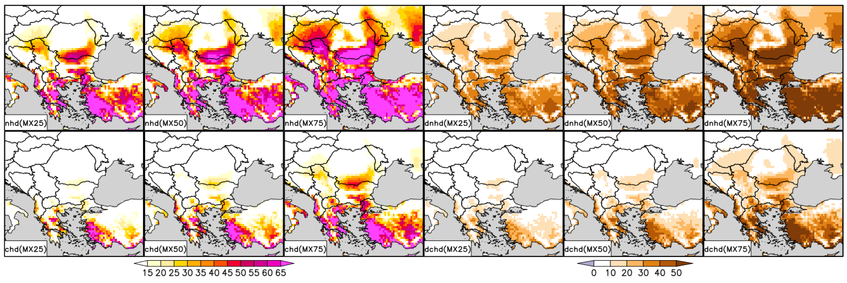
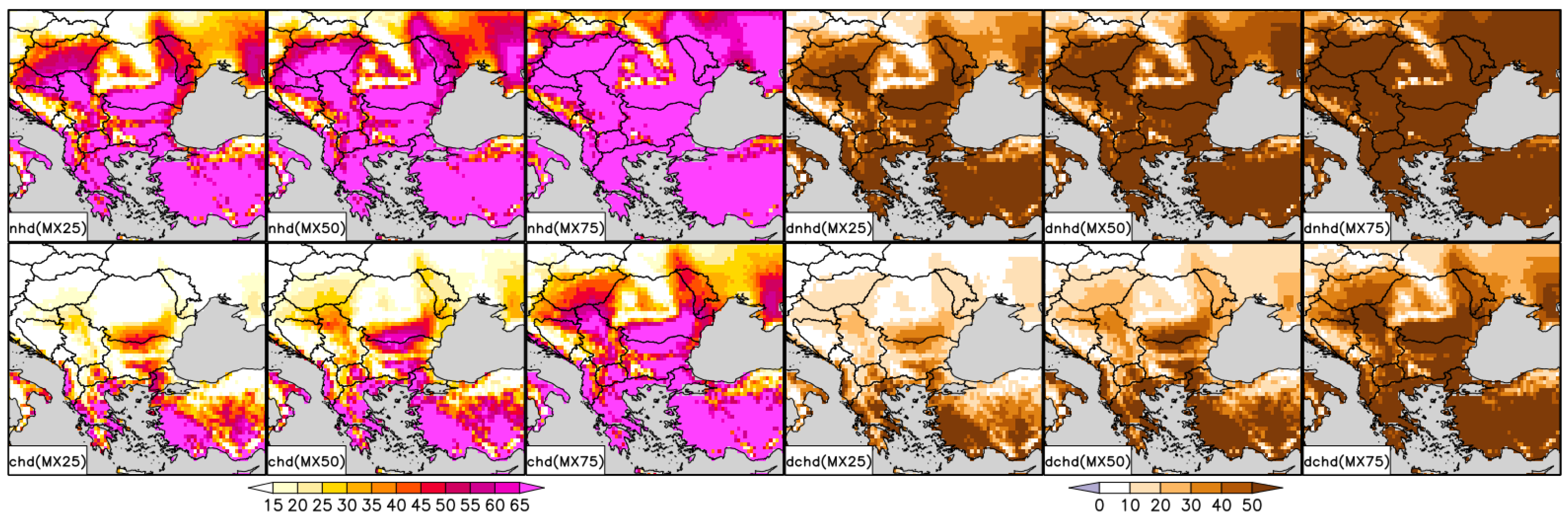
In the next step, we compare the spatial patterns of the multiyear means of the EHEs-indicators in the projected future under both scenarios with their counterparts for the reference period. First, the MME MX25, MX50, and MX75 for the future are compared to the MME MX50 for the reference period, as shown in the case for nhd and chd in Figure 6 for RCP4.5 and in Figure 7 for RCP8.5. The same color legend is used to ensure better comparability between them.
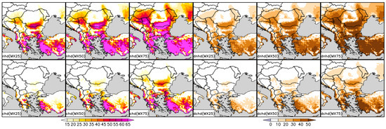
Figure 6.
Multiyear mean values (unit: days) for 2071–2100 under RCP4.5 of the MME MX25, MX50, and MX75 of nhd and chd in the columns 1–3 as well as their differences in respect to multiyear mean values for 1976–2005 of the MME MX50 in columns 4–6.
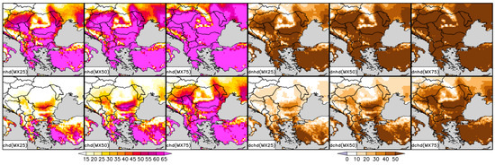
Figure 7.
Multiyear mean values (unit: days) for 2071–2100 under RCP8.5 of the MME MX25, MX50, and MX75 of nhd and chd in the columns 1–3 as well as their differences in respect to multiyear mean values for 1976–2005 of the MME MX50 in columns 4–6.
First and foremost, Figure 6 and Figure 7 show a substantial increase in magnitude and spatial spread of nhd and chd under both scenarios. As a whole, the spatial patterns of EHEs, well evident in the historical period, are preserved. It is worth emphasizing that even the lower MME quartiles (MX25) of chd, especially for nhd, for RCP4.5, are higher than the MME MX50 for 1976–2005 over a large part of the domain. The increase of the multiyear means of the MME MX50 under RCP4.5 in the second period is 30–50 days for nhd and up to 20 days for chd. Correspondingly, these values are more than 50 days and 40–50 days for RCP8.5.
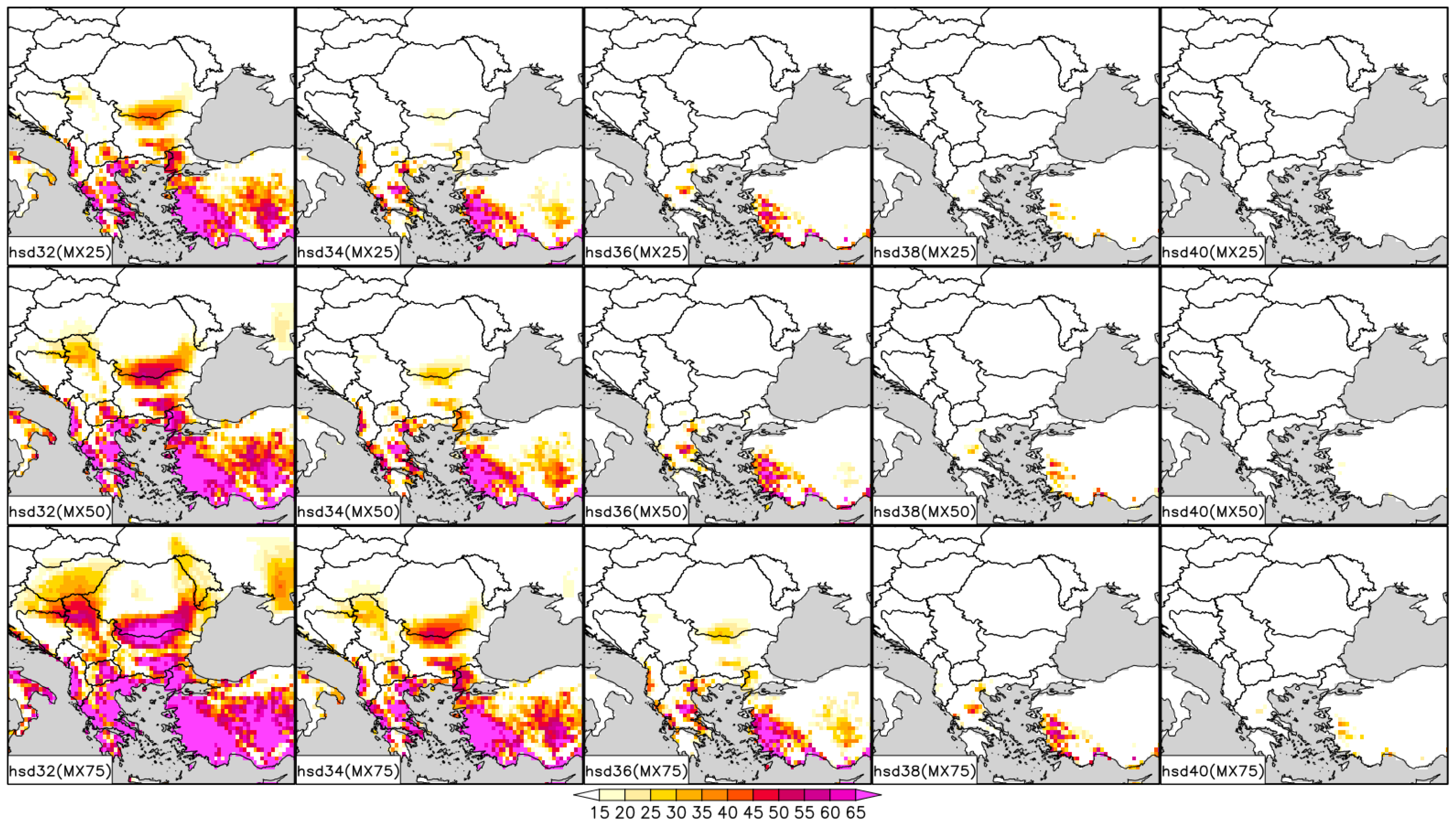
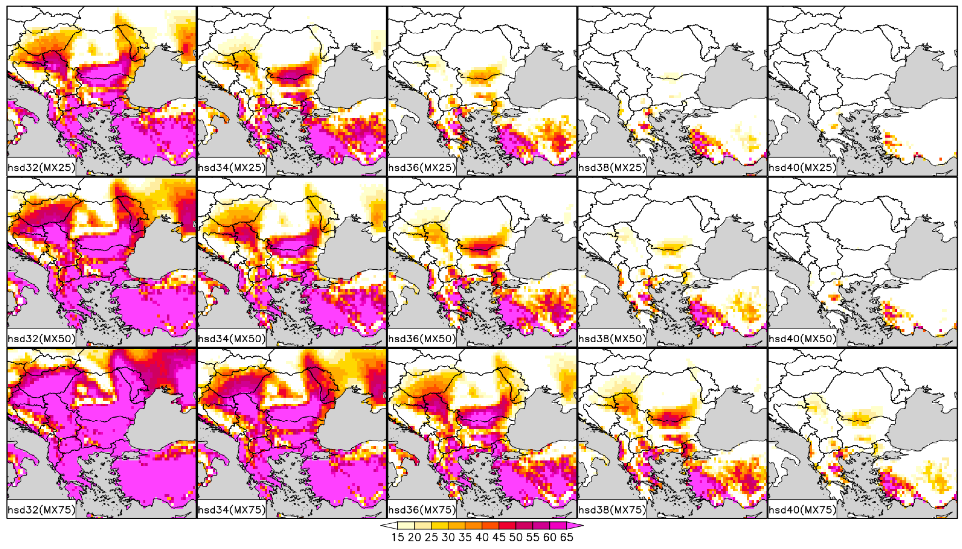
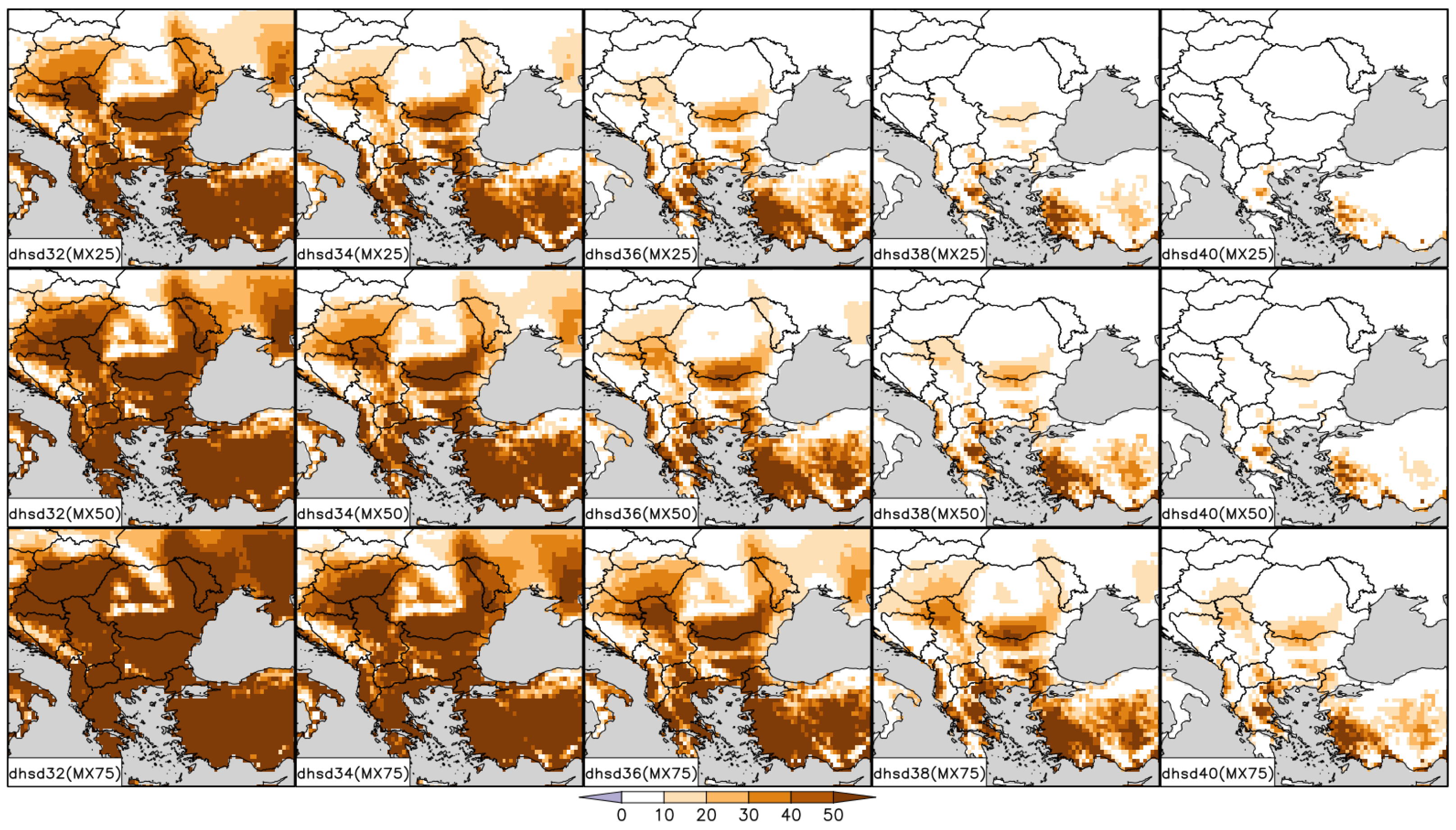
Figure 8 and Figure 9 show the multiyear mean values of MME MX25, MX50, and MX75 of hsd32/34/36/38/40 for 2071–2100 under both scenarios.
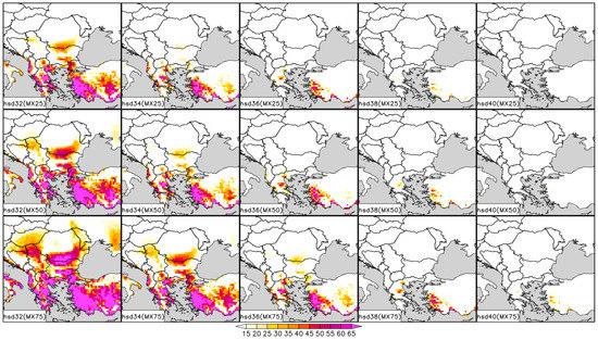
Figure 8.
Multiyear mean values (unit: days) for 2071–2100 under RCP4.5 of the MME MX25, MX50, and MX75 of hsd32/34/36/38/40.
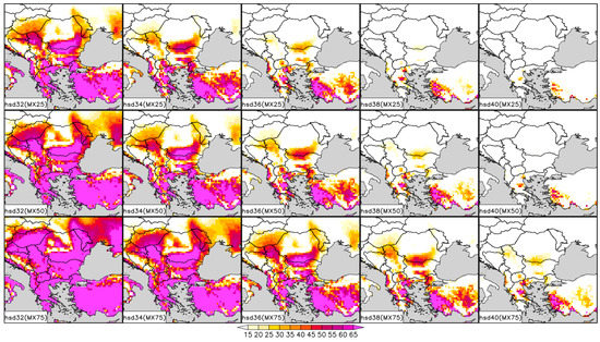
Figure 9.
Multiyear mean values (unit: days) for 2071–2100 under RCP8.5 of the MME MX25, MX50, and MX75 of hsd32/34/36/38/40.
The overall impression of these two figures is their consistency with Figure 6 and Figure 7. Consequently, the outdrawn general conclusions for nhd and chd are also valid for the hsd. As expected, the values of hsd for all thresholds are higher for the scenario with the stronger forcing. The comparison of Figure 8 and Figure 9 with Figure 3 reveals that hsd36/38/40 in the historical period hardly exists. By contrast, for the scenario RCP8.5 in the period of 2071–2100, there is a significant increase in hsd32/34, indicating the direct effect of regional warming in a scenario of comparatively high greenhouse gas emissions [70,72]. The projected long-term means of hsd38/40 would remain close to zero over the bigger part of the domain even by these conditions.
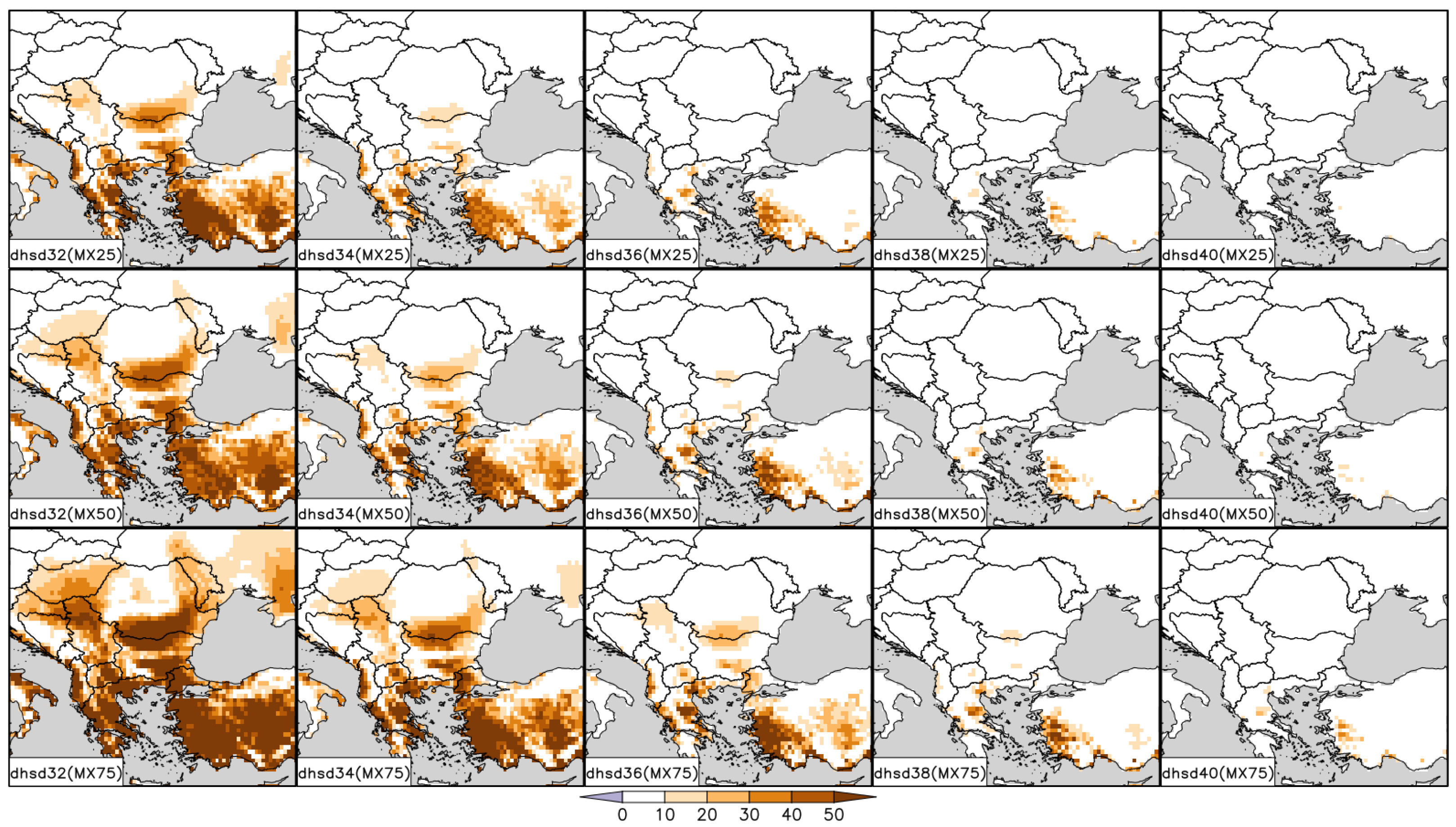
Figure 10 and Figure 11 show differences between the multiyear means of MME MX25, MX50, MX75 of hsd32/34/36/38/40 for 2071–2100 under RCP4.5 and RCP8.5 in respect to the MX50 of the 1976–2005 period.
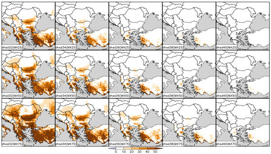
Figure 10.
Differences between the multiyear means of the MME MX25, MX50, MX75 of hsd32/34/36/38/40 for 2071–2100 under RCP4.5 with respect to the MX50 of the 1976–2005 period.

Figure 11.
Differences between the multiyear means of the MME MX25, MX50, MX75 of hsd32/34/36/38/40 for 2071–2100 under RCP8.5 with respect to the MX50 of the 1976–2005 period.
Figure 10 reveals that under RCP4.5, the MX50 of the indicator hsd32 could increase with more than a month over significant parts of Türkiye, Greece, Bulgaria, and the West Balkans. For RCP8.5, (Figure 11) this increase is over 50 days, practically over the whole domain, except for the mountains mainly in Bulgaria (Rila Mountain), the main Carpathian ridge in Romainia and the Dinaric Alps in Croatia and Bosnia and Herzegovina as well as a relatively small area in Slovakia and Poland, close to the northern border. Hence, under RCP4.5 and especially RCP8.5, hsd34 and hsd36 could become meaningful metrics of extreme heat over significant parts of the domain.
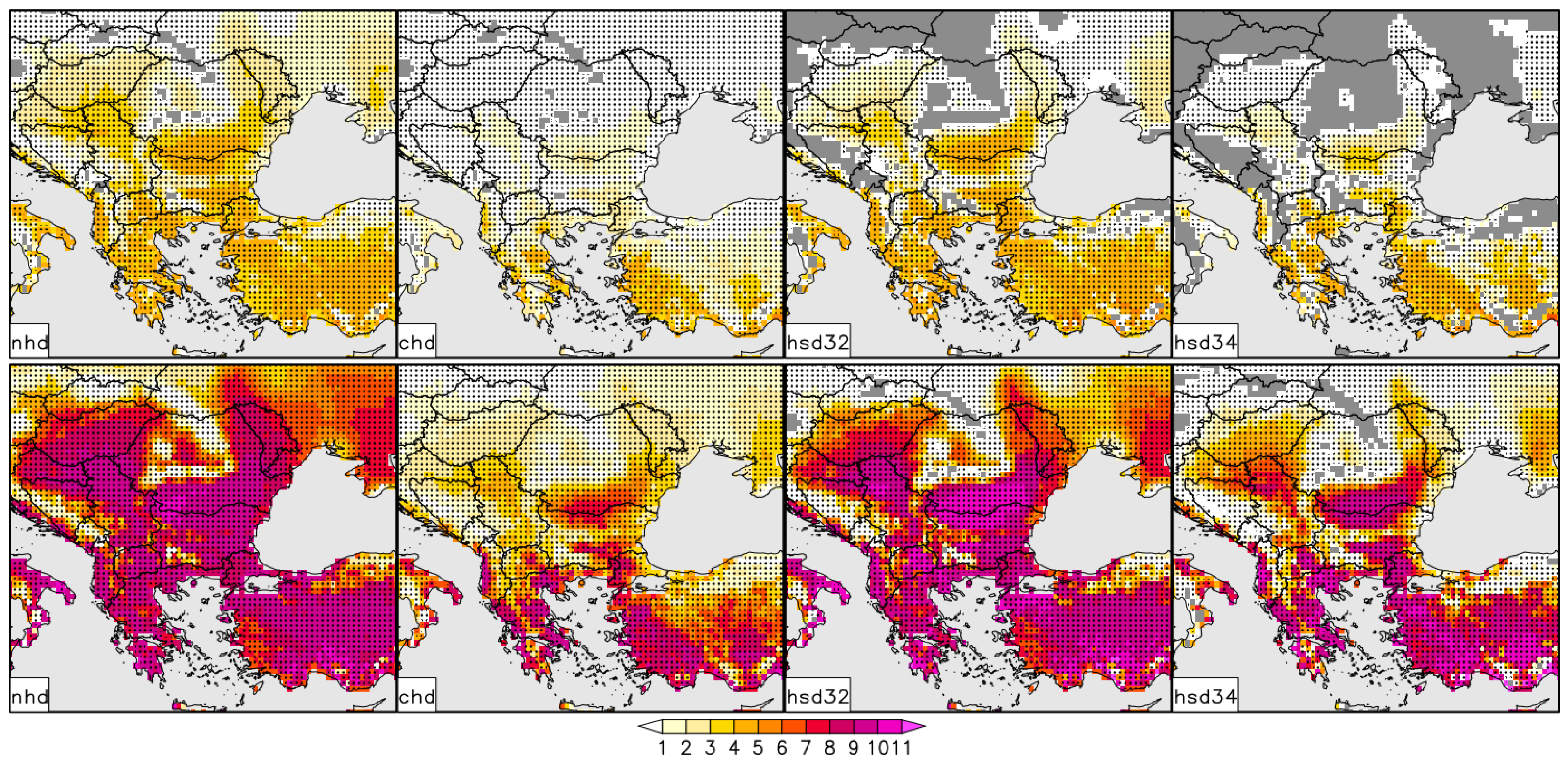
In the present work, the magnitude of the trend is estimated by the Theil-Sen Estimator (TSE) [73,74] and its statistical significance is checked with the Mann-Kendall (MK) test [75,76]. Due to their frequent use in many studies, both methods are practically standard tools for trend analysis in climatology. The trend features are evaluated individually for the time series in every grid cell, as shown in Figure 12, at a 5% significance level (two-tail test).
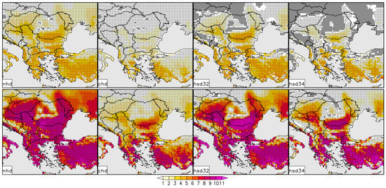
Figure 12.
Trend magnitude (unit: days/10 yr.) of the MME MX50 of the EHEs-indicators according to the column titles under RCP4.5 (first row) and RCP8.5 (second row). Stippling indicates grid cells with significant changes at the 5% significance level.
The trend analysis is implemented only for these land grid cells whose time series are not entirely zero. The areas where annual values of the corresponding indicator are constantly zeros are shown in dark gray. These areas appeared in the mountains and the northern part of the domain. The apparent result of the analysis of Figure 12 is a remarkable difference between RCP4.5 and RCP8.5. Over the bigger part of the domain the trend magnitude is 2–5 days/10 years and 5–10 days/year for RCP4.5 and RCP8.5 correspondingly. Generally, the trend magnitude is twice as large under the scenario with the stronger radiative forcing. The regions with the steepest lapse rate for both scenarios are North Serbia, South Romania - North Bulgaria, continental Greece as well as the biggest part of Türkiye. According to the differences between the EHE-indicators, it is worth to note that the trend magnitude of nhd is essentially larger than this of chd for both scenarios. The same, although not so apparently, is valid for the comparison of hsd32 vs. hsd34 under RCP8.5. As a concluding remark of this section, it is worth emphasizing that in the projected future climate under RCP8.5, the dominating part of the domain, except the high mountains, will become more prone to heat waves.
4. Conclusions
The study utilizes the NEX-GDDP dataset to present the temporal and spatial distribution of regionally tailored extreme heat indicators under two RCP scenarios, RCP4.5 and RCP8.5, until the end of the 21st century. The multi-model ensemble approach is applied, utilizing the complete set of 21 NEX-GDDP GCMs. Overall, the results for the historical period demonstrate that the occurrence of temperature extremes, quantified by the extreme heat indicators, is satisfactorily captured in the NEX-GDDP multi-model ensemble. Consequently, the dataset has the potential to reproduce such extremes in future projections. The study provides clear evidence of a substantial increase in extreme heat events at various temperature thresholds, along with the prolongation of both continuous and non-continuous periods of extreme heat. All of these observed changes are statistically significant. Some of the indicators considered, particularly those related to higher temperature thresholds, are applicable only for a few exceptionally hot years in the historical period (e.g., 1987, 1998, 2000). As a result, their multiyear means are close to zero over a significant part of the domain. However, our results for future projections of the same indicators indicate that they will become meaningful long-term climatological estimators of extreme heat in the second half of the century. Similarly to many other regions worldwide, Southeast Europe is projected to experience more frequent, intense, and prolonged periods of anomalous warmth in the future. This overall pattern closely aligns with the general tendencies of maximum temperature. Although they are based on a novel approach, these key findings are consistent with the main outcomes of recent studies focused on the future climate of the region. As highlighted in previous studies based on NEX-GDDP [45,46], future research could employ a more comprehensive approach based on model data from the ongoing CMIP6 initiative. Such studies could serve as reliable scientific foundations for long-term policy decisions and expert assessments regarding climate extremes and the impacts of climate change.
Author Contributions
Conceptualization, H.C.; methodology, K.M.; software, H.C.; validation, H.C.; formal analysis, K.M.; investigation, K.M.; resources, H.C.; data curation, H.C.; writing—original draft preparation, H.C.; writing—review and editing, K.M.; visualization, K.M.; supervision, K.M. All authors have read and agreed to the published version of the manuscript.
Funding
This research received no external funding.
Institutional Review Board Statement
Not applicable.
Informed Consent Statement
Not applicable.
Data Availability Statement
The NEX-GDDP dataset is free available at: https://www.nccs.nasa.gov/services/data-collections/land-based-products/nex-gddp (accessed on 10 September 2020).
Acknowledgments
Climate scenarios used were from the NEX-GDDP dataset, prepared by the Climate Analytics Group and NASA Ames Research Center using the NASA Earth Exchange, and distributed by the NASA Center for Climate Simulation (NCCS).
Conflicts of Interest
The authors declare no conflict of interest.
Appendix A. NEX-GDDP GCMs

Table A1.
List of the NEX-GDDP GCMs acronyms, institution and country of origin as well as spatial resolution.
Table A1.
List of the NEX-GDDP GCMs acronyms, institution and country of origin as well as spatial resolution.
| GCM | Institution, Country | Resolution (Lon × Lat Levels) |
|---|---|---|
| ACCESSl-0 | Commonwealth Scientific and Industrial Research Organization and Bureau of Meteorology, Australia | 92 × 145 L38 |
| BCC-CSMl-1 | Beijing Climate Center, China Meteorological Administration, China | 128 × 64 L26 (T42) |
| BNU-ESM | Beijing Normal University, China | 128 × 64 L26 (T42) |
| CanESM2 | Canadian Centre for Climate Modelling and Analysis, Canada | 128 × 64 L35 (T63) |
| CCSM4 | National Center for Atmospheric Research (NCAR), USA | 288 × 192 L26 |
| CESMl-BGC | National Science Foundation/Department of Energy NCAR, USA | 288 × 192 L26 |
| CNRM-CM5 | Centre National de Recherches Meteorologiques, Meteo-France, France | 256 × 128 L31 (T127) |
| CSIRO-MK3-6-0 | Australian Commonwealth Scientific and Industrial Research Organization, Australia | 192 × 96 L18 (T63) |
| GFDL-CM3 | Geophysical Fluid Dynamics Laboratory, USA | 144 × 90 L48 |
| GFDL-ESM2G | Geophysical Fluid Dynamics Laboratory, USA | 144 × 90 L24 |
| GFDL-ESM2M | Geophysical Fluid Dynamics Laboratory, USA | 144 × 90 L24 |
| INM-CM4 | Institute for Numerical Mathematics, Russia | 180 × 120 L21 |
| IPSL-CM5A-LR | Institute Pierre-Simon Laplace, France | 96 × 96 L39 |
| IPSL-CM5A-MR | Institute Pierre-Simon Laplace, France | 144 × 143 L39 |
| MIROC-ESM | AORI, NIES, JAMSTEC, Japan | 128 × 64 L80 (T42) |
| MIROC-ESM-CHEM | AORI, NIES, JAMSTEC, Japan | 128 × 64 L80 (T42) |
| MIROC5 | AORI, NIES, JAMSTEC, Japan | 256 × 128 L40 (T85) |
| MPI-ESM-LR | Max Planck Institute for Meteorology, Germany | 192 × 96 L47 (T63) |
| MPI-ESM-MR | Max Planck Institute for Meteorology, Germany | 192 × 96 L95 (T63) |
| MRl-CGCM3 | Meteorological Research Institute, Japan | 320 × 160 L48 (T159) |
| NorESMl-M | Norwegian Climate Centre, Norway | 144 × 96 L26 |
References
- Horton, R.M.; Mankin, J.S.; Lesk, C.; Coffel, E.; Raymond, C. A Review of Recent Advances in Research on Extreme Heat Events. Curr. Clim. Change Rep. 2016, 2, 242–259. [Google Scholar] [CrossRef]
- Sun, Q.; Miao, C.; Hanel, M.; Borthwick, A.G.L.; Duan, Q.; Ji, D.; Li, H. Global Heat Stress on Health, Wildfires, and Agricultural Crops under Different Levels of Climate Warming. Environ. Int. 2019, 128, 125–136. [Google Scholar] [CrossRef] [PubMed]
- Harkness, C.; Semenov, M.A.; Areal, F.; Senapati, N.; Trnka, M.; Balek, J.; Bishop, J. Adverse Weather Conditions for UK Wheat Production under Climate Change. Agric. For. Meteorol. 2020, 282–283, 107862. [Google Scholar] [CrossRef]
- Hatfield, J.L.; Prueger, J.H. Temperature Extremes: Effect on Plant Growth and Development. Weather. Clim. Extrem. 2015, 10, 4–10. [Google Scholar] [CrossRef]
- WMO. The Global Climate 2001–2010, a Decade of Climate Extremes; WMO-No. 1103; WMO: Geneva, Switzerland, 2013; p. 119. [Google Scholar]
- Schoetter, R.; Cattiaux, J.; Douville, H. Changes of Western European Heat Wave Characteristics Projected by the CMIP5 Ensemble. Clim. Dyn. 2015, 45, 1601–1616. [Google Scholar] [CrossRef]
- Spinoni, J.; Vogt, J.V.; Barbosa, P.; Dosio, A.; McCormick, N.; Bigano, A.; Füssel, H.-M. Changes of Heating and Cooling Degree-Days in Europe from 1981 to 2100: HDD and CDD in Europe from 1981 to 2100. Int. J. Climatol. 2018, 38, e191–e208. [Google Scholar] [CrossRef]
- Coccolo, S.; Kämpf, J.; Scartezzini, J.; Pearlmutter, D. Outdoor human comfort and thermal stress: A comprehensive review on models and standards. Urban Clim. 2016, 18, 33–57. [Google Scholar] [CrossRef]
- Vandentorren, S.; Bretin, P.; Zeghnoun, A.; Mandereau-Bruno, L.; Croisier, A.; Cochet, C.; Ribéron, J.; Siberan, I.; Declercq, B.; Ledrans, M. August 2003 Heat Wave in France: Risk Factors for Death of Elderly People Living at Home. Eur. J. Public Health 2006, 16, 583–591. [Google Scholar] [CrossRef] [PubMed]
- Gao, M.; Yang, J.; Gong, D.; Shi, P.; Han, Z.; Kim, S.-J. Footprints of Atlantic Multidecadal Oscillation in the Low-Frequency Variation of Extreme High Temperature in the Northern Hemisphere. J. Clim. 2019, 32, 791–802. [Google Scholar] [CrossRef]
- Perkins, S.E.; Alexander, L.V.; Nairn, J.R. Increasing Frequency, Intensity and Duration of Observed Global Heatwaves and Warm Spells. Geophys. Res. Lett. 2012, 39, 2012GL053361. [Google Scholar] [CrossRef]
- Vautard, R.; van Aalst, M.; Boucher, O.; Drouin, A.; Haustein, K.; Kreienkamp, F.; van Oldenborgh, G.J.; Otto, F.E.L.; Ribes, A.; Robin, Y.; et al. Human contribution to the record-breaking June and July 2019 heatwaves in Western Europe. Environ. Res. Lett. 2020, 15, 094077. [Google Scholar] [CrossRef]
- Becker, F.N.; Fink, A.H.; Bissolli, P.; Pinto, J.G. Towards a More Comprehensive Assessment of the Intensity of Historical European Heat Waves (1979–2019). Atmos. Sci. Lett. 2022, 23, e1120. [Google Scholar] [CrossRef]
- Morabito, M.; Crisci, A.; Messeri, A.; Messeri, G.; Betti, G.; Orlandini, S.; Raschi, A.; Maracchi, G. Increasing Heatwave Hazards in the Southeastern European Union Capitals. Atmosphere 2017, 8, 115. [Google Scholar] [CrossRef]
- Russo, S.; Sillmann, J.; Fischer, E.M. Top ten European heatwaves since 1950 and their occurrence in the coming decades. Environ. Res. Lett. 2015, 10, 124003. [Google Scholar] [CrossRef]
- Beniston, M. The 2003 heatwave in Europe: A shape of things to come? An analysis based on Swiss climatological data and model simulations: The 2003 heat wave in Europe. Geophys. Res. Lett. 2004, 31. [Google Scholar] [CrossRef]
- Barriopedro, D.; Fischer, E.M.; Luterbacher, J.; Trigo, R.M.; García-Herrera, R. The Hot Summer of 2010: Redrawing the Temperature Record Map of Europe. Science 2011, 332, 220–224. [Google Scholar] [CrossRef]
- Sánchez-Benítez, A.; García-Herera, R.; Barriopedro, D.; Sousa, P.M.; Trigo, R.M. June 2017: The Earliest European Summer Megaheatwave of Reanalysis Period. Geophys. Res. Lett. 2018, 45, 1955–1962. [Google Scholar] [CrossRef]
- Masson-Delmotte, V.; Zhai, P.; Pirani, A.; Connors, S.; Péan, C.; Berger, S.; Caud, N.; Chen, Y.; Goldfarb, L.; Gomis, M.; et al. Climate Change 2021: The Physical Science Basis. In Contribution of Working Group I to the Sixth Assessment Report of the Intergovernmental Panel on Climate Change; Technical Report; IPCC: Geneva, Switzerland, 2021. [Google Scholar]
- Kostopoulou, E.; Jones, P.D. Assessment of climate extremes in the Eastern Mediterranean. Meteorol. Atmos. Phys. 2005, 89, 69–85. [Google Scholar] [CrossRef]
- Alexandrov, V.; Schneider, M.; Koleva, E.; Moisselin, J.M. Climate variability and change in Bulgaria during the 20th century. Theor. Appl. Climatol. 2004, 79, 133–149. [Google Scholar] [CrossRef]
- Philandras, C.M.; Nastos, P.T.; Repapis, C.C. Air temperature variability and trends over Greece. Glob. Nest J. 2008, 10, 273–285. [Google Scholar]
- Toreti, A.; Desiato, F.; Fioravanti, G.; Perconti, W. Seasonal temperatures over Italy and their relationship with low-frequency atmospheric circulation patterns. Clim. Change 2008, 99, 211–227. [Google Scholar] [CrossRef]
- Bartolini, G.; di Stefano, V.; Maracchi, G.; Orlandini, S. Mediterranean warming is especially due to summer season - evidences from Tuscany (central Italy). Theor. Appl. Climatol. 2012, 107, 279–295. [Google Scholar] [CrossRef]
- Xoplaki, E.; González-Rouco, J.; Gyalistras, D.; Luterbacher, J.; Rickli, R.; Wanner, H. Interannual summer air temperature variability over Greece and its connection to the large-scale atmospheric circulation and Mediterranean SSTs 1950–1999. Clim. Dyn. 2003, 20, 537–554. [Google Scholar] [CrossRef]
- Lhotka, O.; Kyselý, J. The 2021 European Heat Wave in the Context of Past Major Heat Waves. Earth Space Sci. 2022, 9, e2022EA002567. [Google Scholar] [CrossRef]
- Xoplaki, E.; Trigo, R.M.; García-Herrera, R.; Barriopedro, D.; D’Andrea, F.; Fischer, E.M.; Gimeno, L.; Gouveia, C.; Hernández, E.; Kuglitsch, F.G.; et al. Large-Scale Atmospheric Circulation Driving Extreme Climate Events in the Mediterranean and Its Related Impacts. In The Climate of the Mediterranean Region; Elsevier: Amsterdam, The Netherlands, 2012; pp. 347–417. ISBN 9780124160422. [Google Scholar] [CrossRef]
- Lelieveld, J.; Hadjinicolaou, P.; Kostopoulou, E.; Chenoweth, J.; El Maayar, M.; Giannakopoulos, C.; Hannides, C.; Lange, M.A.; Tanarhte, M.; Tyrlis, E.; et al. Climate change and impacts in the Eastern Mediterranean and the Middle East. Clim. Chang. 2012, 114, 667–687. [Google Scholar] [CrossRef] [PubMed]
- Molina, M.O.; Sánchez, E.; Gutiérrez, C. Future heat waves over the Mediterranean from an Euro-CORDEX regional climate model ensemble. Sci Rep. 2020, 10, 8801. [Google Scholar] [CrossRef]
- Giorgi, F. Climate change hot-spots. Geophys. Res. Lett. 2006, 33, L08707. [Google Scholar] [CrossRef]
- Diffenbaugh, N.S.; Pal, J.S.; Giorgi, F.; Gao, X. Heat stress intensification in the Mediterranean climate change hotspot. Geophys. Res. Lett. 2007, 34, 1–6. [Google Scholar] [CrossRef]
- Seneviratne, S.I.; Zhang, X.; Adnan, M.; Badi, W.; Dereczynski, C.; Di Luca, A.; Vicente-Serrano, S.M.; Wehner, M.; Zhou, B. Weather and Climate. In Climate Change 2021: The Physical Science Basis. Contribution of Working Group I to the Sixth Assessment Report of the Intergovernmental Panel on Climate Change; IPCC: Geneva, Switzerland, 2021; pp. 1513–1766. [Google Scholar] [CrossRef]
- Cramer, W.; Guiot, J.; Fader, M.; Garrabou, J.; Gattuso, J.-P.; Iglesias, A.; Lange, M.A.; Lionello, P.; Llasat, M.C.; Paz, S.; et al. Climate Change and Interconnected Risks to Sustainable Development in the Mediterranean. Nat. Clim Chang. 2018, 8, 972–980. [Google Scholar] [CrossRef]
- Taylor, K.E.; Stouffer, R.J.; Meehl, G.A. An Overview of CMIP5 and the Experiment Design. Bull. Am. Meteorol. Soc. 2012, 93, 485–498. [Google Scholar] [CrossRef]
- Raghavan, S.V.; Hur, J.; Liong, S.-Y. Evaluations of NASA NEX-GDDP Data over Southeast Asia: Present and Future Climates. Clim. Chang. 2018, 148, 503–518. [Google Scholar] [CrossRef]
- Sillmann, J.; Kharin, V.V.; Zwiers, F.W.; Zhang, X.; Bronaugh, D. Climate Extremes Indices in the CMIP5 Multimodel Ensemble: Part 2. Future Climate Projections. J. Geophys. Res. Atmos. 2013, 118, 2473–2493. [Google Scholar] [CrossRef]
- Meehl, G.A.; Tebaldi, C. More Intense, More Frequent, and Longer Lasting Heat Waves in the 21st Century. Science 2004, 305, 994–997. [Google Scholar] [CrossRef]
- Wobus, C.; Zarakas, C.; Malek, P.; Sanderson, B.; Crimmins, A.; Kolian, M.; Sarofim, M.; Weaver, C.P. Reframing Future Risks of Extreme Heat in the United States. Earth’s Future 2018, 6, 1323–1335. [Google Scholar] [CrossRef] [PubMed]
- Jacob, D.; Petersen, J.; Eggert, B.; Alias, A.; Christensen, O.B.; Bouwer, L.M.; Braun, A.; Colette, A.; Déqué, M.; Georgievski, G.; et al. EURO-CORDEX: New High-Resolution Climate Change Projections for European Impact Research. Reg. Environ. Change 2014, 14, 563–578. [Google Scholar] [CrossRef]
- Parker, W.S. Ensemble Modeling, Uncertainty and Robust Predictions. WIREs Clim. Change 2013, 4, 213–223. [Google Scholar] [CrossRef]
- Jain, S.; Salunke, P.; Mishra, S.K.; Sahany, S.; Choudhary, N. Advantage of NEX-GDDP over CMIP5 and CORDEX Data: Indian Summer Monsoon. Atmos. Res. 2019, 228, 152–160. [Google Scholar] [CrossRef]
- Merrifield, A.L.; Brunner, L.; Lorenz, R.; Medhaug, I.; Knutti, R. An Investigation of Weighting Schemes Suitable for Incorporating Large Ensembles into Multi-Model Ensembles. Earth Syst. Dynam. 2020, 11, 807–834. [Google Scholar] [CrossRef]
- Herger, N.; Abramowitz, G.; Knutti, R.; Angélil, O.; Lehmann, K.; Sanderson, B.M. Selecting a Climate Model Subset to Optimise Key Ensemble Properties. Earth Syst. Dynam. 2018, 9, 135–151. [Google Scholar] [CrossRef]
- Ali, J.; Syed, K.H.; Gabriel, H.F.; Saeed, F.; Ahmad, B.; Bukhari, S.A.A. Centennial Heat Wave Projections Over Pakistan Using Ensemble NEX GDDP Data Set. Earth Syst. Environ. 2018, 2, 437–454. [Google Scholar] [CrossRef]
- Cao, N.; Li, G.; Rong, M.; Yang, J.; Xu, F. Large Future Increase in Exposure Risks of Extreme Heat Within Southern China Under Warming Scenario. Front. Earth Sci. 2021, 9, 686865. [Google Scholar] [CrossRef]
- Luo, Z.; Yang, J.; Gao, M.; Chen, D. Extreme Hot Days over Three Global Mega-regions: Historical Fidelity and Future Projection. Atmos. Sci. Lett. 2020, 21, e1003. [Google Scholar] [CrossRef]
- Chervenkov, H.; Slavov, K. NEX-GDDP Multimodel Ensemble vs. E-OBS—Evaluation of the Extreme Temperatures and Precipitation over Southeast Europe: Historical Comparison. Atmosphere 2022, 13, 581. [Google Scholar] [CrossRef]
- Malcheva, K.; Bocheva, L.; Chervenkov, H. Spatio-Temporal Variation of Extreme Heat Events in Southeastern Europe. Atmosphere 2022, 13, 1186. [Google Scholar] [CrossRef]
- Malcheva, K.; Bocheva, L.; Chervenkov, H. Climatology of extremely hot spells in bulgaria (1961–2019). In Proceedings of the 21st International Multidisciplinary Scientific GeoConference SGEM (2021), SPA Albena Complex, Bulgaria, 26 June–5 July 2021; pp. 311–318. [Google Scholar] [CrossRef]
- Kottek, M.; Grieser, J.; Beck, C.; Rudolf, B.; Rubel, F. World Map of the Köppen-Geiger climate classification updated. Meteorol. Z. 2006, 15, 259–263. [Google Scholar] [CrossRef] [PubMed]
- Lionello, P.; Abrantes, F.; Congedi, L.; Dulac, F.; Gacic, M.; Gomis, D.; Goodess, C.; Hoff, H.; Kutiel, H.; Luterbacher, J.; et al. Introduction: Mediterranean Climate-Background Information. In The Climate of the Mediterranean Region; Elsevier: Amsterdam, The Netherlands, 2012; p. xxxv–xc. [Google Scholar] [CrossRef]
- Cornes, R.C.; Van Der Schrier, G.; Van Den Besselaar, E.J.M.; Jones, P.D. An Ensemble Version of the E-OBS Temperature and Precipitation Data Sets. J. Geophys. Res. Atmos. 2018, 123, 9391–9409. [Google Scholar] [CrossRef]
- Kotlarski, S.; Keuler, K.; Christensen, O.B.; Colette, A.; Déqué, M.; Gobiet, A.; Goergen, K.; Jacob, D.; Lüthi, D.; Van Meijgaard, E.; et al. Regional Climate Modeling on European Scales: A Joint Standard Evaluation of the EURO-CORDEX RCM Ensemble. Geosci. Model Dev. 2014, 7, 1297–1333. [Google Scholar] [CrossRef]
- Thrasher, B.; Maurer, E.P.; McKellar, C.; Duffy, P.B. Technical Note: Bias Correcting Climate Model Simulated Daily Temperature Extremes with Quantile Mapping. Hydrol. Earth Syst. Sci. 2012, 16, 3309–3314. [Google Scholar] [CrossRef]
- Meinshausen, M.; Smith, S.J.; Calvin, K.; Daniel, J.S.; Kainuma, M.L.T.; Lamarque, J.-F.; Matsumoto, K.; Montzka, S.A.; Raper, S.C.B.; Riahi, K.; et al. The RCP Greenhouse Gas Concentrations and Their Extensions from 1765 to 2300. Clim. Change 2011, 109, 213–241. [Google Scholar] [CrossRef]
- Thomson, A.M.; Calvin, K.V.; Smith, S.J.; Kyle, G.P.; Volke, A.; Patel, P.; Delgado-Arias, S.; Bond-Lamberty, B.; Wise, M.A.; Clarke, L.E.; et al. RCP4.5: A pathway for stabilization of radiative forcing by 2100. Clim. Change 2011, 109, 77–94. [Google Scholar] [CrossRef]
- Riahi, K.; Rao, S.; Krey, V.; Cho, C.; Chirkov, V.; Fischer, G.; Kindermann, G.; Nakicenovic, N.; Rafaj, P. RCP 8.5—A scenario of comparatively high greenhouse gas emissions. Clim. Change 2011, 109, 33–57. [Google Scholar] [CrossRef]
- Maurer, E.P.; Hidalgo, H.G. Utility of daily vs. monthly large-scale climate data: An intercomparison of two statistical downscaling methods. Hydrol. Earth Syst. Sci. 2008, 12, 551–563. [Google Scholar] [CrossRef]
- Chadalavada, K.; Gummadi, S.; Kundeti, K.R.; Kadiyala, D.M.; Deevi, K.C.; Dakhore, K.K.; Bollipo Diana, R.K.; Thiruppathi, S.K. Simulating Potential Impacts of Future Climate Change on Post-Rainy Season Sorghum Yields in India. Sustainability 2021, 14, 334. [Google Scholar] [CrossRef]
- Kumar, P.; Kumar, S.; Barat, A.; Sarthi, P.P.; Sinha, A.K. Evaluation of NASA’s NEX-GDDP-Simulated Summer Monsoon Rainfall over Homogeneous Monsoon Regions of India. Theor. Appl. Climatol. 2020, 141, 525–536. [Google Scholar] [CrossRef]
- Bao, Y.; Wen, X. Projection of China’s near- and Long-Term Climate in a New High-Resolution Daily Downscaled Dataset NEX-GDDP. J. Meteorol. Res. 2017, 31, 236–249. [Google Scholar] [CrossRef]
- Perkins, S.E.; Alexander, L.V. On the Measurement of Heat Waves. J. Clim. 2013, 26, 4500–4517. [Google Scholar] [CrossRef]
- Nairn, J.; Fawcett, R. The Excess Heat Factor: A Metric for Heatwave Intensity and Its Use in Classifying Heatwave Severity. Int. J. Environ. Res. Public Health 2014, 12, 227–253. [Google Scholar] [CrossRef]
- WMO. Guidelines on the Definition and Characterization of Extreme Weather and Climate Events; WMO-No. 1310; WMO: Geneva, Switzerland, 2023; ISBN 978-92-63-11310-8. [Google Scholar]
- Schulzweida, U. CDO User Guide. 2020. [Google Scholar] [CrossRef]
- Willmott, C.J.; Ackleson, S.G.; Davis, R.E.; Feddema, J.J.; Klink, K.M.; Legates, D.R.; O’Donnell, J.; Rowe, C.M. Statistics for the Evaluation and Comparison of Models. J. Geophys. Res. 1985, 90, 8995. [Google Scholar] [CrossRef]
- Jose, D.M.; Vincent, A.M.; Dwarakish, G.S. Improving Multiple Model Ensemble Predictions of Daily Precipitation and Temperature through Machine Learning Techniques. Sci. Rep. 2022, 12, 4678. [Google Scholar] [CrossRef]
- Krause, P.; Boyle, D.P.; Bäse, F. Comparison of Different Efficiency Criteria for Hydrological Model Assessment. Adv. Geosci. 2005, 5, 89–97. [Google Scholar] [CrossRef]
- Prado, R.C.D.; Blain, G.C.; Picoli, M.C.A. Rainfall Data from the European Center for Medium-Range Weather Forecast for Monitoring Meteorological Drought in the State of São Paulo. Acta Sci. Technol. 2018, 40, 34947. [Google Scholar] [CrossRef]
- Chervenkov, H.; Slavov, K. Theil-Sen Estimator vs. Ordinary Least Squares—Trend Analysis for Selected ETCCDI Climate Indices. Comptes Rendus Acad. Bulg. Sci. 2019, 72, 47–54. [Google Scholar] [CrossRef]
- Zhang, X.; Alexander, L.; Hegerl, G.C.; Jones, P.; Tank, A.K.; Peterson, T.C.; Trewin, B. and Zwiers, F.W. Indices for monitoring changes in extremes based on daily temperature and precipitation data. WIREs Clim Change 2011, 2, 851–870. [Google Scholar] [CrossRef]
- Chervenkov, H.; Ivanov, V.; Gadzhev, G.; Ganev, K. Assessment of the Future Climate over Southeast Europe Based on CMIP5 Ensemble of Climate Indices—Part Two: Results and Discussion. In Proceedings of the 1st International Conference on Environmental Protection and Disaster Risks, Sofia, Bulgaria, 29–30 September 2020. [Google Scholar] [CrossRef]
- Theil, H. A rank-invariant method of linear and polynomial regression analysis. I, II, III. Nederl. Akad. Wetensch. Proc. 1950, 53, 386–392, 521–525, 1397–1412. [Google Scholar]
- Sen, P.K. Estimates of the regression coefficient based on Kendall’s tau. J. Am. Stat. Assoc. 1968, 63, 1379–1389. [Google Scholar] [CrossRef]
- Mann, H.B. Nonparametric Tests against Trend. Econometrica 1945, 13, 245–259. [Google Scholar] [CrossRef]
- Kendall, M.G. A New Measure of Rank Correlation. Biometrika 1938, 30, 81–93. [Google Scholar] [CrossRef]
Disclaimer/Publisher’s Note: The statements, opinions and data contained in all publications are solely those of the individual author(s) and contributor(s) and not of MDPI and/or the editor(s). MDPI and/or the editor(s) disclaim responsibility for any injury to people or property resulting from any ideas, methods, instructions or products referred to in the content. |
© 2023 by the authors. Licensee MDPI, Basel, Switzerland. This article is an open access article distributed under the terms and conditions of the Creative Commons Attribution (CC BY) license (https://creativecommons.org/licenses/by/4.0/).

