Article

Study of Time-Frequency Domain Characteristics of the Total Column Ozone in China Based on Wavelet Analysis

1
School of Electrical & Information Engineering, Anhui University of Science and Technology, Huainan 232001, China
2
State Key Laboratory of Space Weather, Chinese Academy of Sciences, Beijing 100190, China
3
School of Internet, Anhui University, Hefei 230039, China
*
Author to whom correspondence should be addressed.
Atmosphere 2023, 14(6), 941; https://doi.org/10.3390/atmos14060941
Submission received: 17 April 2023 / Revised: 16 May 2023 / Accepted: 25 May 2023 / Published: 27 May 2023
(This article belongs to the Section Atmospheric Techniques, Instruments, and Modeling)

Abstract

:
Ozone is a very important trace gas in the atmosphere, it is like a “double-edged sword”. Because the ozone in the stratosphere can effectively help the earth’s organisms to avoid the sun’s ultraviolet radiation damage, the ozone near the ground causes pollution. Therefore, it is essential to explore the time-frequency domain variation characteristics of total column ozone and have a better understanding of its cyclic variation. In this paper, based on the monthly scale dataset of total column ozone (TCO) (September 2002 to February 2023) from Atmospheric Infrared Sounder (AIRS) carried by NASA’s Aqua satellite, linear regression, coefficient of variation, Mann-Kendall (M-K) mutation tests, wavelet analysis, and empirical orthogonal function decomposition (EOF) analysis were used to analyze the variation characteristics of the TCO in China from the perspectives of time domain, frequency domain, and spatial characteristics. Finally, this study predicted the future of TCO data based on the seasonal autoregressive integrated moving average (SARIMA) model in the time series algorithm. The results showed the following: (1) From 2003 to 2022, the TCO in China showed a slight downward trend, with an average annual change rate of −0.29 DU/a; the coefficient of variation analysis found that TCO had the smallest intra-year fluctuations in 2008 and the largest intra-year fluctuations in 2005. (2) Using the M-K mutation test, it was found that there was a mutation point in the total amount of column ozone in 2016. (3) Using wavelet analysis to analyze the frequency domain characteristics of the TCO, it was observed that TCO variation in China had a combination of 14-year, 6-year, and 4-year main cycles, where 14 years is the first main cycle with a 10-year cycle and 6 years is the second main cycle with a 4-year cycle. (4) The spatial distribution characteristics of the TCO in China were significantly different in each region, showing a distribution characteristic of being high in the northeast and low in the southwest. (5) Based on the EOF analysis of the TCO in China, it was found that the variance contribution rate of the first mode was as high as 52.85%, and its spatial distribution of eigenvectors showed a “-” distribution. Combined with the trend analysis of the time coefficient, this showed that the TCO in China has declined in the past 20 years. (6) The SARIMA model with the best parameters of (1, 1, 2) × (0, 1, 2, 12) based on the training on the TCO data was used for prediction, and the final model error rate was calculated as 1.34% using the mean absolute percentage error (MAPE) index, indicating a good model fit.

1. Introduction

Ozone is a very important trace gas in the atmosphere; approximately 90% of the ozone in the atmosphere is concentrated in the stratosphere 10–40 km above the earth’s surface [1], and the remaining ozone is located in the troposphere [2]. It is like a “double-edged sword”—why do we think so? Because ozone in the stratosphere can protect any organisms on the earth’s surface from harmful solar ultraviolet medium- (UVB) and short-wave (UVC) radiation, but in the troposphere, it is a strong greenhouse gas. Although the concentration of ozone in the troposphere is lower than that in the stratosphere, it is an important source of hydroxyl radicals, which are powerful oxidants that can break down various pollutants and easily react with other chemicals to produce toxic oxides and other greenhouse gases; thus, increases in ozone at these altitudes can lead to climate change [3,4]. Especially since the discovery of the Antarctic ozone hole in the mid-1980s, the importance of ozone in the atmosphere has been known to the public, and the hole in the ozone layer directly threatens the survival of human beings on Earth [5]. Therefore, in 1987, the “Montreal Protocol on Substances that Deplete the Ozone Layer” formally identified chlorofluorocarbons (CFCs) and other ozone-depleting substances (ODCs) as a major threat to the ozone layer, marking the beginning of a concerted international effort to reduce and eventually phase out the global production and consumption of ODCs [6].
Ozone has a very significant impact on our lives. Therefore, research on ozone is not only of scientific value but also closely related to the daily life of human beings. Academic studies of whole-layer ozone use the column concentration method to represent the distribution of ozone, and, in this paper, we use TCO as an abbreviation for total column ozone. For scholars at home and abroad, related research on the ozone problem has increasingly become a very important scientific research topic. Zhang, J.Q. et al. [7] quantified the vertical ozone variability at different time scales using ozone data from Dobson measurements in the downtown Beijing and Xianghe suburban areas and found that the ozone single-peak and Dobson-based total column ozone exhibited consistent sinusoidal monthly variations, with a maximum value of 380 Dobson units (DU) in March and a minimum value of 305 DU in October. Based on the global TCO data of a global multi-sensor reanalysis (MSR2), Zhou, P. et al. [8] studied the temporal and spatial variation characteristics of TCO in the Yangtze River Delta region of China from 2000 to 2019 and the correlation between it and related meteorological factors, populations, and industrial output values. They found that TCO is significantly higher in spring than in other seasons and the correlation between annual changes of TCO and meteorological factors is weak, indicating that it is affected by the game interaction of different external driving factors. Bian, J.C. et al. [9] analyzed the cause of the summer ozone trough on the Qinghai-Tibet Plateau using total column ozone daily product data provided by the ozone monitoring instrument (OMI) on the Aura spacecraft, one of the NASA EOS platforms, and found that it was mainly caused by the Asian summer monsoon (ASM) and changes in the air column over the plateau. Zhang, J.K. et al. [10] investigated the long-term trends and influencing factors of TCO on the Tibetan Plateau from 1979 to 2009 using total ozone mapping spectrometer/solar backscatter UV radiometer (TOMS/SBUV) combined TCO data, and the analysis showed that TCO on the Tibetan Plateau was greatly correlated with increases in upper-layer temperature. Chidinma, O.E. et al. [11] mainly studied the influence of solar and geomagnetic activities on the total column ozone in three major cities in Northern, Eastern, and Southern China. The monthly/annual direct forcing response of the surface sun and the geomagnetic storm index had a prominent impact on TCO. They found that TCO varies depending on the phase of the solar cycle. Okoro, E.C. et al. [12] studied the response of total atmospheric ozone to solar activity over China’s Mountain Waliguan and analyzed its periodic changes. The analysis found that there is a clear and continuous seasonal pattern in the total column ozone, and its maximum values occur in winter/spring, while the minimum values occur in summer/autumn. They also found that the ozone over China’s Mountain Waliguan is in a recovery phase.
At the same time, computer technology has developed rapidly in recent years, and various machine learning and neural network algorithms have emerged in an endless stream. These algorithms are widely used in geography, oceanography, and meteorology, among other fields. Therefore, using big data and machine learning algorithms to process and analyze collected weather data can be more efficient than traditional methods to solve research problems. This new interdisciplinary scientific research method has become the mainstream development trend of the future. For example, Wang, S. et al. [13] used a new deep learning model based on convolutional neural network architecture to estimate the ground ozone concentration in Eastern China. Compared with commonly used machine learning methods, the accuracy of the model was improved. It provided more accurate data for atmospheric environment research. Zou, M. et al. [14] used the ensemble empirical mode decomposition (EEMD) algorithm to trend three datasets, including TCO products of the OMI (ozone detector) in the Tibetan Plateau region, and found that the average annual growth rate of TCO from 2004 to 2019 was 0.377 DU/a and the average annual growth rate of ozone deficiency events was 0.263 DU/a.
In summary, domestic and foreign scholars have more often studied a local area alone or a country as a whole to analyze the characteristics of change from a spatial and temporal perspective. Based on this, this study not only analyzes changes in the characteristics of the TCO in China as a whole but also takes into account an analysis of seven specific geographical regions of China. Secondly, this study introduces wavelet transform, an algorithm in the field of signal processing, to study the frequency domain features behind time domain variations, taking into account traditional spatiotemporal feature analysis. The article concludes with an analysis of the correlations between TCO and influencing factors such as SO2 and NOx emissions from exhaust gas emissions. Therefore, this paper is a study of TCO variation and local zoning characteristics in China from the perspective of time, frequency, and spatial domains. We conclude our paper by considering the seasonal characteristics of TCO predicted by an algorithmic model. After reviewing the data, we found that Valipour M et al. [15] used autoregressive integrated moving average (ARIMA) and SARIMA models for long-term runoff prediction comparison, and their study concluded that SARIMA models have better accuracy for predicting data with periodic characteristics. Therefore, this study makes a short-term prediction based on the SARIMA model, an algorithm suitable for seasonal time series data, which helps to provide some reference for future studies related to the TCO in the Chinese region.

2. Data Sources and Methods

2.1. Data Introduction

The TCO dataset used in this study was provided by the Atmospheric Infrared Sounder (AIRS) carried by NASA’s Aqua satellite, which has been in a sun-synchronous polar orbit since May 2002 [16]. The current versions of data detected by AIRS include V5, V6, and V7 [17], which mainly provide datasets of meteorological factors such as ozone, long-wave radiation flux, and temperature within the troposphere [6]. The TCO data used in this study were obtained from AIRS Version6 Level3 monthly product data (time range: September 2002 to February 2022), and the data precision was 1° × 1° (latitude × longitude).
Data on impact factors related to TCO change used in this paper include NOx emissions from exhaust gases; SO2 emissions data were all downloaded from the database of the National Bureau of Statistics of China.

2.2. Introduction of Research Methods

2.2.1. Linear Regression

This paper used linear regression in a machine learning algorithm to fit the trend of the relationship between two sets of variables. The expression of linear regression model is as follows:
y = k x + b
The two sets of variables are x and y in the expression, such as the trend of satellite ozone data over time fitted with a linear regression model in Section 3.1 of this paper, where k represents the rate of change, k > 0 means that the data y increases with x and vice versa, and b is the intercept of the equation.

2.2.2. Pearson Correlation Coefficient

In this study, the correlation coefficient RXY was used to measure the correlation between two sets of variables, X and Y, where RXY takes values in the range [−1,1]. When RXY is closer to 1, the stronger the positive correlation is between two sets of variables, X and Y; conversely, the closer RXY is to −1, the stronger the negative correlation is, and the closer RXY is to 0, the weaker the correlation is [18].
R X Y = i = 1 N X i X ¯ Y i Y ¯ i = 1 N X i X ¯ 2 i = 1 N Y i Y ¯ 2

2.2.3. Coefficient of Variation

The coefficient of variation (CV) is the ratio between the standard deviation (σ) of a segment of data and the arithmetic mean of the data (μ); it is calculated as follows:
C V = σ μ
The standard deviation (σ) is calculated as follows:
σ = i = 1 N X i X ¯ 2 N
The average value (μ) is calculated as follows:
μ = i = 1 N X i N
N in Equations (4) and (5) is the overall amount of data, X i is the i-th sample of data in the overall sample of data, and X ¯ is the arithmetic mean of the overall sample of data.
In this study, the temporal coefficients of variation on annual and multi-year monthly mean scales were used to analyze the fluctuation in TCO data in a certain time domain. Compared with the standard deviation, it avoids the influence of the magnitude and measurement scales and can better reflect the degree of fluctuation of the data itself.

2.2.4. Mann-Kendall Mutation Test

The Mann-Kendall mutation test is a non-parametric statistical test method, also known as the non-distribution test, which can be used to detect the monotonic trend direction of time series data [19]. Currently, this method is widely used in related fields such as meteorological data time series analysis, and it is also easy to implement with many programming languages such as Python, Matlab, etc. In this study, the Mann-Kendall mutation test was implemented in Python language. Since it considers the ordering of observations rather than actual values, it is less affected by the actual distribution and less sensitive to outliers.
UF is a forward TCO time series curve, and UB is the reverse TCO time series curve, which is the opposite of UF. If the UF value is greater than 0, this indicates that the series shows an upward trend; if it is less than 0, this indicates that the series shows a downward trend. When values exceed the critical confidence level, this indicates a clear upward or downward trend, and the time node above the critical line is the time region where the mutation occurs. If the intersection point of the two curves of UF and UB is between the critical lines, then the moment corresponding to the intersection point is the time when the mutation starts; if the intersection point is outside the critical lines, or if there is more than one clear intersection point, it is not clear where the mutation point is.

2.2.5. Wavelet Analysis

Jean Morlet was the first author to use the word wavelet [20]. He understood that the window length of short-time Fourier transform (STFT) was fixed, making it difficult to meet the requirements of diverse frequency domain feature analysis; thus, he improved it to a transform with an adjustable window length, which is called a Morlet wavelet today. Changes in common meteorological element data are often influenced by several factors; thus, their change characteristics pattern is more complex. The TCO studied in this paper is no exception, and Morlet wavelet analysis was introduced to investigate the phenomenon of periodic variation of frequency domain characteristics.
This type of analysis can clearly reveal various change cycles hidden in time series and fully reflect the change trend of a system under different time scales. Wavelet analysis mainly uses the localization characteristics of the wavelet function in the time and frequency domains to reveal multi-level variation rules of data [21]. The wavelet function is expressed as follows:
+ Ψ t d t = 0 , Ψ t L 2 ( R )
Ψ t is the wavelet basis function, whose function system is represented as follows:
Ψ a , b t = | a | 1 / 2 Ψ t b a a , b R , a 0
Ψ a , b t is the daughter wavelet; a is the scale factor, which reflects the period length of the wavelet function; and b is the displacement factor, which reflects the shift of the wavelet function in time.

2.2.6. EOF (Empirical Orthogonal Function Decomposition) Analysis

EOF analysis (the empirical orthogonal function decomposition method) was invented by Pearson (1901). Since its introduction into meteorology by Lorenz (1956), the method has been widely used by meteorologists and oceanographers to analyze the spatial and temporal variability of physical fields [22]. EOF analysis, also known as principal component analysis, is an algorithm whose main objective is to find a new set of orthogonal empirical functions by reorganizing the original dataset. These new orthogonal functions are linearly transformed from the original dataset and are ordered by decreasing variance. The first orthogonal function represents the maximum variation in the original dataset; the second contributes more to the original dataset than the subsequent function, and so on. Thus, this recombination minimizes the root mean square error (RMSE) of the reconstruction results using a given number of empirical orthogonal functions [23].

2.2.7. Time Series Forecasting Algorithm SARIMA Model

The seasonal autoregressive integrated moving average (SARIMA) model is used in Section 3.4 of this study for the prediction of the TCO in the Chinese region.
The modeling process of the SARIMA model is as follows:
(1)
Test the data for smoothness by the augmented Dickey–Fuller (ADF) test to determine whether the data meet the smoothness requirement. (The ADF test can be used to test whether the current series is smooth. P-value is one of the parameters used to determine whether the data are smooth or not. If the p-value is less than 0.05, the original hypothesis can be rejected [24], the data do not have a unit root, and the series is smooth; if it is greater than or equal to 0.05, the original hypothesis cannot be significantly rejected and the next step of judgment is required.)
(2)
Plot the data time series, observe its seasonal characteristics, determine the seasonal characteristic period s of the data, and eliminate the seasonal characteristics of the data by seasonal differencing (s-order differencing).
(3)
Draw auto- and bias correlation diagrams and determine the approximate parameter value range by observing these two diagrams.
(4)
Use the iterative method and Akaike information criterion (AIC) to determine the optimal parameters and use the optimal parameters to train the model to complete the modeling (for a detailed explanation of the AIC, see [25]).
(5)
Perform a residual test on the established model to test the model fit.
(6)
Perform forecasting by using the model and conducting error rate analysis using the MAPE index.

2.3. Data Validation

The reliability of the AIRS dataset used in this paper was verified using data from three atmospheric background stations in the northern hemisphere, and the validation part included month-by-month comparison analyses and correlation tests.
The three atmospheric local station datasets used in this paper were obtained from the Earth System Research Laboratory (ESRL) of NOAA (National Oceanic and Atmospheric Administration). The sites selected for comparison were Boulder, Colorado (BLD), United States; the Barrow Atmospheric Baseline Observatory (BRW), United States; and Haute Provence, France (OHP). Detailed information about sites is shown in Table 1.
The monthly mean data from the AIRS were selected for correlation analysis with the data from the Boulder background station, the Barrow Atmosphere Baseline Observatory, and the Provence base station during the same time period, and the Pearson correlation coefficients were 0.9509, 0.9771, and 0.9403, respectively (see Figure 1). Statistically speaking, when the correlation coefficient between two variables was between 0.8 and 1, the correlation between them was extremely strong. That is, the data from the two data sources showed a strong correlation with each other. Therefore, from the results of the analysis, it could be concluded that the AIRS data had certain reliability.

3. Results

3.1. Analysis of the Time-Frequency Domain Variation of Regional TCO in China

3.1.1. Analysis of the Interannual Variation of Regional TCO in China

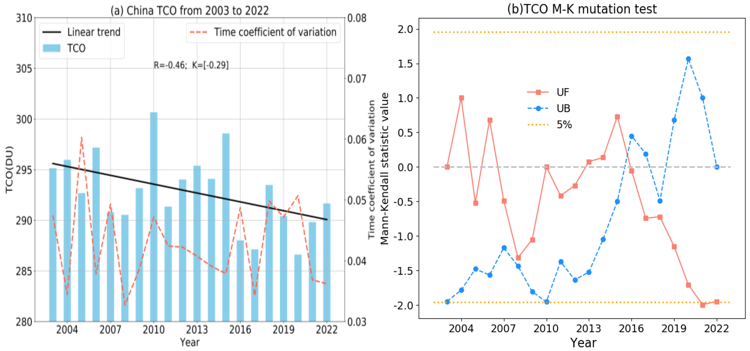
The annual mean analysis of the TCO data obtained by AIRS yielded Figure 2a, which shows the interannual variation characteristics of total ozone in the Chinese region during 2003–2022. First, a linear regression model was used to fit the trend in total ozone over these 20 years, and the fitted regression model equation was Y = [−0.29] X + 879, which meant that the regression coefficient was −0.29 and the intercept was 879. That is, the linear regression analysis yielded an overall slope K value of −0.29 from 2003 to 2022, which meant that the annual decrease in total ozone was 0.29 (DU), meaning that the overall trend over the last 20 years has been decreasing, though the trend is small. From a TCO of 295.1 DU in 2003 with a time variation coefficient of 0.047 at the beginning, it finally reached 291.7 DU in 2022, with the time variation coefficient decreasing to 0.036. This means that the average total ozone has decreased by 3.4 DU in 20 years, and fluctuations within the year have also been reduced. From the results of the analysis of the temporal coefficient of variation for each year, the intra-year fluctuation was the smallest in 2008, with a coefficient of variation of 0.033, and it was the largest in 2005, with a coefficient of variation of 0.06. That is, the degree of fluctuation in 2005 was 1.8 times greater than that in 2008. The mean time coefficient of variation from 2003 to 2022 was 0.043.
Then, we used the M–K mutation test method to test the annual average data of these 20 years. The UF curve is the forward time series curve of the total annual average ozone in China and the UB is the reverse time series curve; the inside of the two dashed lines is the 95% significance test range. Observing Figure 2b, UF > 0 in 2004 and 2006 and from 2014 to 2016, indicating an upward trend in the TCO during this period; UF < 0 from 2016 to 2022, indicating a decrease in the TCO during this period. In general, the value of the UF curve from 2003 to 2022 was less than 0 most of the time, indicating that the results of the previous analysis of the downward trend of TCO in China from 2003 to 2022 are reliable. There was an intersection point between the UF and UB curves around 2016, and the intersection point was within the significance test range; thus, it was determined that TCO experienced a mutation around 2016.

3.1.2. Analysis of Monthly Variation of TCO in China

As Figure 3a shows the time series of monthly data of the TCO in the Chinese region from September 2002 to February 2023, it can be observed that the periodic characteristics of the TCO are still very clear and that the cycle was a cycle of approximately 12 months. Figure 3b shows the multi-year monthly average variation of TCO in China (September 2002~February 2023), where the coefficient of temporal variation is the ratio of the standard deviation of the multi-year monthly scale mean total ozone in the Chinese region from September 2002 to February 2023 to the multi-year monthly scale mean, which was used to describe the data fluctuation in multi-year monthly mean TCO.
From the results of the analysis, it is clear that there is indeed a significant time-domain variation in the multi-year monthly average TCO in the Chinese region, and the monthly average TCO shows a characteristic like a “sine curve” with the variation of the monthly scale. Figure 3b shows that the peak of the annual ozone column occurred in April with a peak value of 307.3 DU and the trough occurred in November with a trough value of 276.7 DU, which is a difference of 30.6 DU. Observing Figure 3b, the low-value area lasted from October to December. The TCO increased significantly from January onwards and the TCO remained at a relatively high-value domain from January onwards. TCO in moderate latitudes is strongly dependent on meridional Brewer–Dobson circulation [26] because ozone is mainly produced in the tropics and transported through the atmospheric circulation to the middle and high latitudes [27,28]. The pattern of changes in total ozone reflects the depletion of ozone from April to November due to the dominant role of photochemical losses when solar radiation is strong; the rest of the time, it was in a state of accumulation [29]. This can be observed starting in November and then in January, February, and March when TCO was in a growth phase.
Second, this paper introduces the time variation coefficient to analyze the fluctuation of the monthly mean TCO data over many years. Judging from the time variation coefficient analysis results, the fluctuation in the TCO in February was the greatest, with a time variation coefficient of 0.03, and the fluctuation in the July data was the smallest, with a time variation coefficient of 0.018. That is, the degree of volatility in July was only approximately 60% of that in February. The fluctuation in monthly average ozone values varied considerably from month to month. From a seasonal perspective, it can be observed that the fluctuation in TCO change was the smallest in autumn and the greatest in winter, and the fluctuation degree in TCO changes over the four seasons was ranked as follows: winter > spring > summer > autumn.

3.1.3. Seasonal Variation Analysis of TCO in China

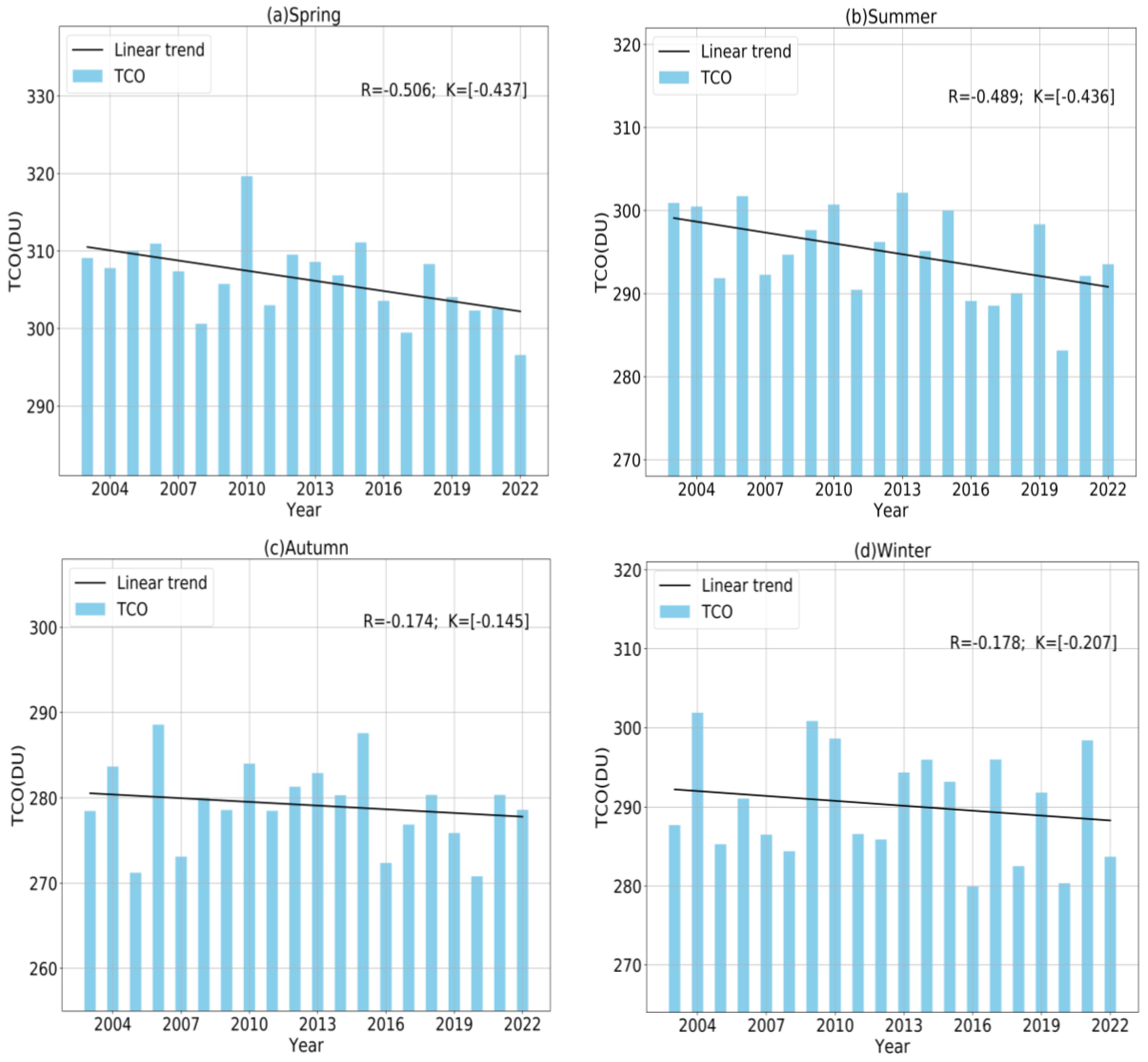
In order to better analyze the changes in the total regional ozone column in China, this paper separately analyzes the changes in the seasonal annual averages for the four seasons from 2003 to 2022. In this paper, March, April, and May of each year are designated as spring; June, July, and August are designated as summer; September, October, and November are designated as autumn; and December and January and February of the following year are designated as winter of the previous year. As shown in Figure 4, the interannual variation of ozone column content in the Chinese region was analyzed for the four seasons. The overall ozone column content in spring was the highest among the four seasons over the last 20 years in terms of the total amount, with a mean value of 306 DU; the annual average ozone column concentration in autumn was relatively the lowest, reaching 279 DU. The order of TCO size in four seasons was spring > summer > winter > autumn. This paper used linear regression to analyze the trend of TCO in each season during this period. R refers to the correlation coefficient and K represents the average annual variation of ozone column content under that season. When K > 0, it means that the trend increased with time and if K < 0, it menas that it decreased with time. The TCO in the four seasons over the past 20 years had a slight downward trend as a whole, but the rate of change varied greatly. The TCO in spring experienced the fastest decline among the four seasons (K = −0.437), that is, the annual seasonal mean of the spring TCO in China decreased at a rate of −0.437 DU per year; in autumn, the TCO experienced the slowest decline (K = −0.145). The order of the overall decline rate of the four seasons was spring > summer > winter > autumn.

3.1.4. Frequency Domain Analysis of TCO in China

While the above analysis examined the variation pattern of the regional TCO in China from a time domain perspective, this section further explores the cyclical pattern behind the hidden time domain variation phenomenon. Therefore, a better research tool is to introduce frequency domain analysis algorithms to solve such problems. In this paper, wavelet analysis algorithms in the field of information and signal processing were used to study the periodicity of TCO data.
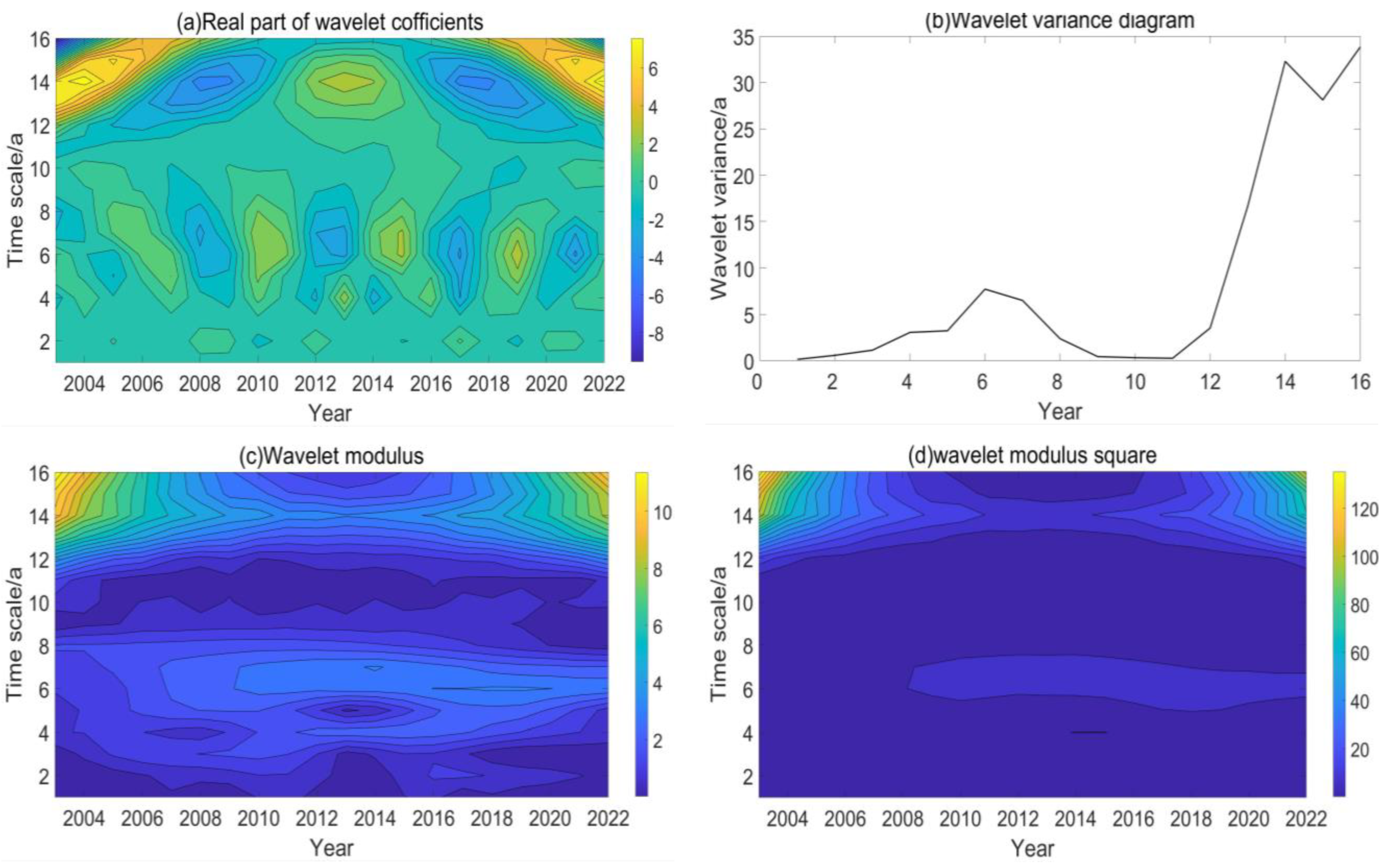
Figure 5 shows the wavelet transform analysis of the TCO in China from 2003 to 2022, from which it can be observed that the variation of the TCO in China was characterized by the phenomenon of nested cycles at different time scales. The implication is that there was not only a cycle in the variation of the TCO in some specific time periods but that the cycle itself also had a cyclic variation. It can be observed from Figure 5a that the TCO in China did have main cycles of 4~6 and 14~16 years. The distribution of the fluctuation energy of the TCO time series with the time scale reflected by the variance diagram of the wavelet analysis in Figure 5b more accurately reflects the main cycle that existed in the change process of the TCO. As shown in Figure 5b, there were two more distinct peaks in the wavelet square difference curve of the TCO, which corresponded to the 14- and 6-year time scales, in turn. As can be observed from Figure 5b, the largest peak corresponded to the 14-year time scale, which reflected the strongest fluctuation in the cycle change of 14 years as the first main cycle of the total regional ozone column change in China. The 6-year time scale corresponded to the second peak, which was the second main cycle of the total regional ozone column variation in China. Combined with the above analysis, it can also be observed from the wavelet modulus value diagram in Figure 5c and wavelet modulus square diagram in Figure 5d that the energy spectrum was more clear at the time scales of 14 and 6 years; thus, the previous analysis verified the correctness of the main cycle situation.
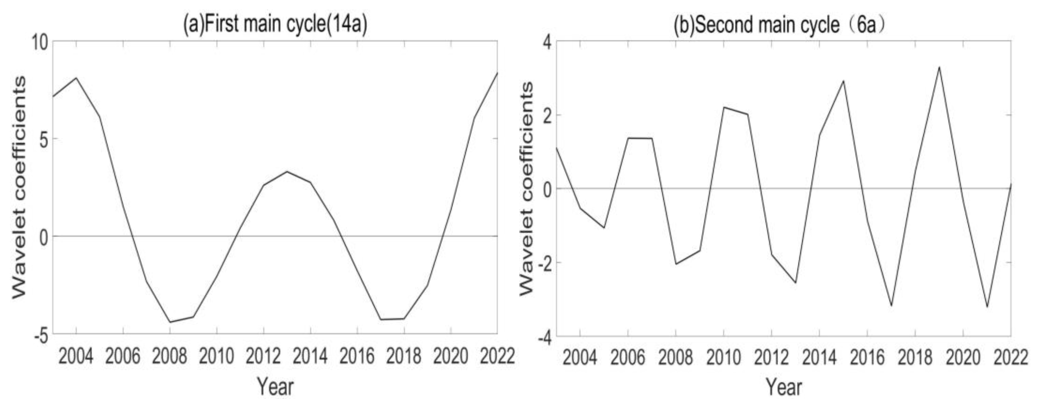
The so-called main cycle was the time scale selected before the cycle change was observed because different cycle changes may be characterized at different time scales. Therefore, according to the results of the main cycles analyzed above, the time scales of the first and second main cycles were selected in turn, and the wavelet coefficient maps corresponding to the multi-scale features were drawn. As shown in Figure 6, it is clear that there were different periodic changes under different time scales.
Figure 6a shows that the change cycle of the TCO in China amounted to approximately 10 years, corresponding to 14 years as the first main cycle, and approximately two cycles were experienced from 2003 to 2022. Figure 6b shows that when 6 years accounted for the second main cycle scale, the corresponding change cycle of the TCO in China was approximately 4 years, and approximately five cycles were experienced from 2003 to 2022.

3.2. Spatial Distribution of TCO in China

3.2.1. Spatial Distribution Characteristics of Annual Mean TCO in China

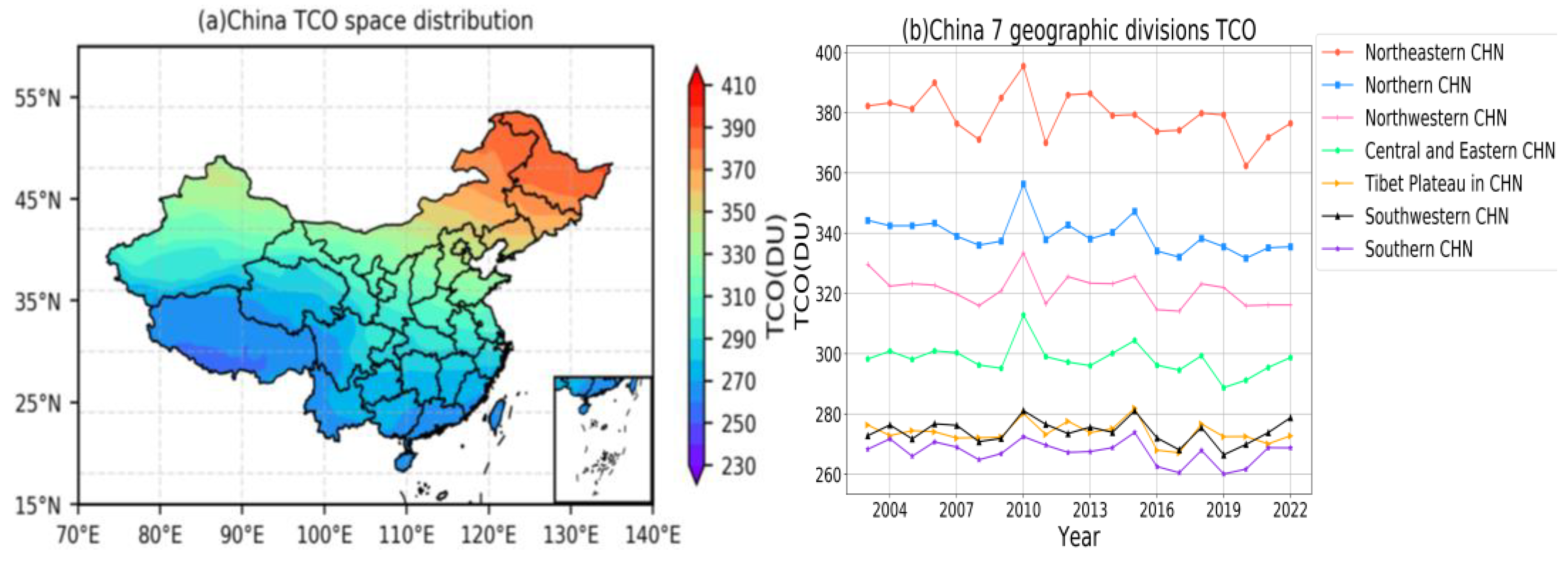
The TCO dataset of the Chinese region from September 2002 to February 2023 provided by AIRS was selected, and this dataset was processed by multi-year averaging and data gridding using a Python program to plot the spatial distribution of the TCO in the Chinese region for the past 20 years (see Figure 7a). The figure shows clear differences in the characteristics of the TCO in different regions of China, with higher TCO in the northeastern region and lower TCO in the Qinghai-Tibet Plateau region and Southern China, with the maximum value occurring in the northeastern region at approximately 385 DU and the minimum value occurring in the southwest of Qinghai-Tibet region at approximately 260 DU.
After conducting the above-mentioned spatial analysis of the TCO in China, the spatial distribution characteristics of the average value of the TCO in China in the past 20 years could be roughly clarified. In order to more clearly observe the long-term characteristics of the spatial distribution of each division, China was divided into Northeastern China (118° E~135° E, 41° N~53.55° N), Northern China (110° E~120° E, 35° N~45° N), Central and Eastern China (113° E~125° E, 27° N~37° N), Qinghai-Tibet Plateau (73° E~104° E, 28° N~38° N), Southwestern China (97° E~110° E, 21° N~33° N), Northwestern China (73°E~110° E, 35° N~50° N), and Southern China (104.5° E~117° E, 18° N~27° N) to conduct a long-term comparative analysis of the above partitions.
As shown in Figure 7b, China was divided into seven regions, and the interannual variation of the TCO in the seven regions was analyzed. The general trend of the rise and fall in the seven regions was similar over the period 2003 to 2022. Among them, from 2001 to 2008, the overall trend in Northeastern China, Northern China, Northwestern China, and Central and Eastern China declined, while the trend in the Qinghai-Tibet Plateau region, Southwestern China, and Southern China was relatively stable. The trend was on the rise from 2008 to 2010, and all the above seven regions reached their maximum in 2010. After 2010, the seven major regions all experienced a relatively clear decline in 2011, and then from 2012 to 2022, the seven regions generally returned to relatively stable trends, and some regions showed a weak downward trend. This is consistent with the previous conclusions in the time series analysis of China as a whole.
Analyzing the change in the TCO over many years, the TCO has been higher in Northeastern China and Northern China in the past 20 years, while the Qinghai-Tibet Plateau region and Southern China have been in the lower value area.

3.2.2. Seasonal Spatial Distribution Characteristics of TCO in China

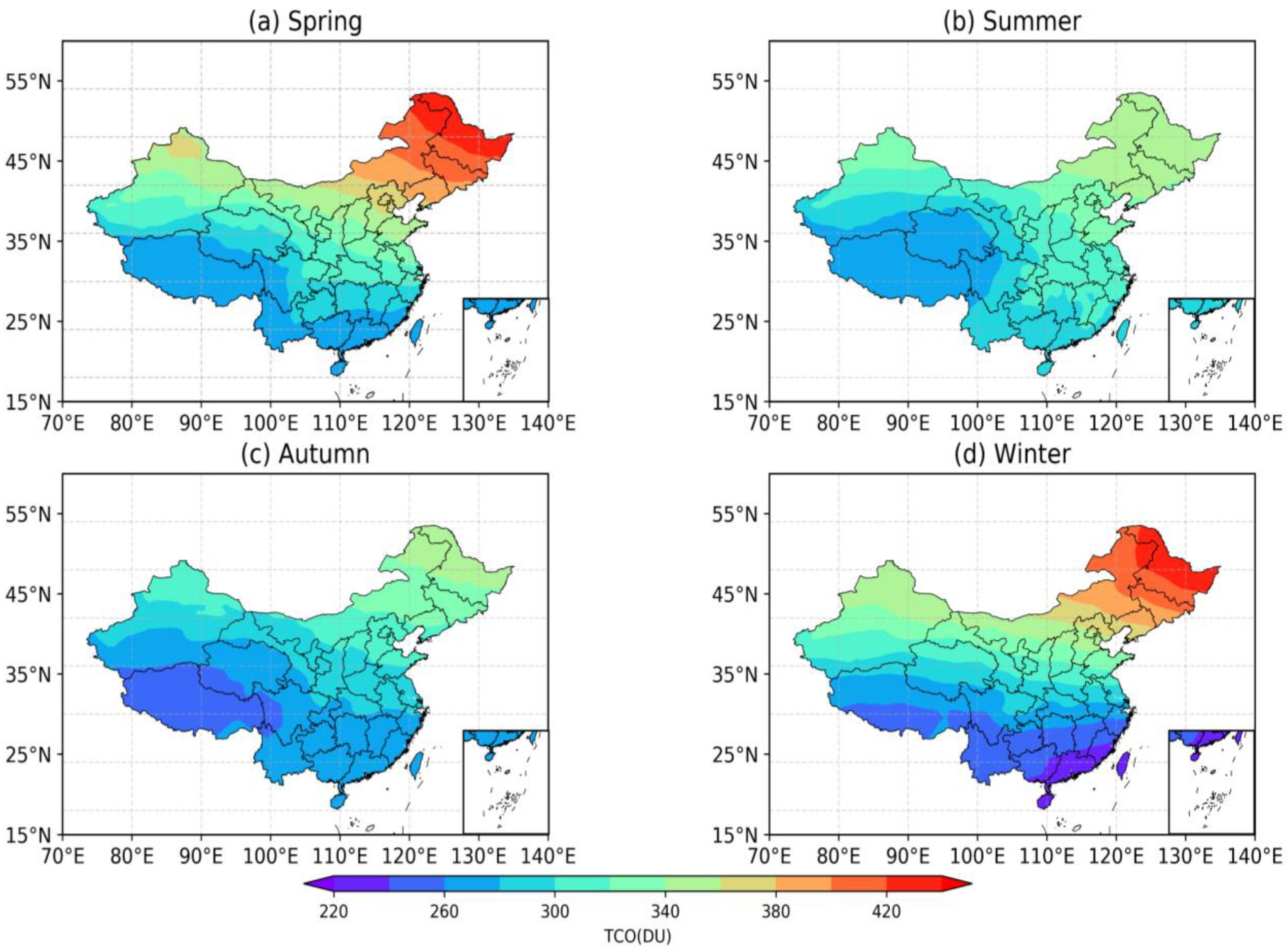
We selected the average spatial and temporal data of ozone column content from March to May for each year for data analysis and visual display to obtain the multi-year spring average spatial distribution of China’s TCO. Similarly, the average spatiotemporal data of TCO from June to August were selected as the spatial distribution of TCO in summer. The average spatiotemporal data of TCO in China from September to November were selected as the spatial distribution in autumn. The average time and space data of TCO in China from December to February of the next year were selected as the spatial distribution map of TCO in winter.
As shown in Figure 8, the seasonal differences in the TCO in China were clear. The overall distribution of the TCO in autumn was the lowest among the four seasons of the year, while the TCO in spring was the highest, which is consistent with the previous findings from the analysis of the total ozone in the multi-year mean change of the four seasons from the time domain perspective. The seasonal cycle characteristics of TCO were mainly affected by photochemical reactions and power transportation, in which solar radiation was one of the components of photochemical reactions, which directly affected the consumption and production of ozone [27,28,29,30].
It was also found that the TCO in Northeast China had the highest value in the whole Chinese region in all four seasons, and the lowest values were observed in Southern China and the Qinghai-Tibet Plateau region. The latitudinal difference in TCO distribution in winter was the most clear, while the latitudinal difference in the overall distribution of TCO in summer was relatively unclear. Over the four overall seasonal distribution maps, it was also found that the TCO in the northeastern region was higher overall, while the TCO in the Qinghai-Tibet Plateau region was lower almost all year round; thus, the issue of low ozone values in the Qinghai-Tibet Plateau region is always a hot topic. A review of relevant data revealed that the problem of low ozone values in the Qinghai-Tibet Plateau region may be related to its unique topography and the shortening of the ozone column due to high altitude. Examining the distribution of the TCO in the whole of China, from northeast to southwest, as the latitude decreases, the total ozone also shows a decreasing trend.
In order to further analyze the relationship between TCO and latitude and longitude, the distribution of the ozone column versus latitude and longitude was plotted. As shown in Figure 9a, the TCO in China increased with increasing latitude, especially after 30° N. The increasing trend was more clear.
Finally, examining the plot of TCO versus longitude in Figure 9b, we can observe that the curve is similar to a “V” shape, with a clear difference in the trend between the two sides of longitude 90° E. In the longitude range from approximately 70° E to 90° E, the TCO decreases with increasing longitude and then generally shows an increasing trend between approximately longitude 90° E and 130° E.

3.2.3. EOF Analysis of Temporal and Spatial Characteristics of TCO in China

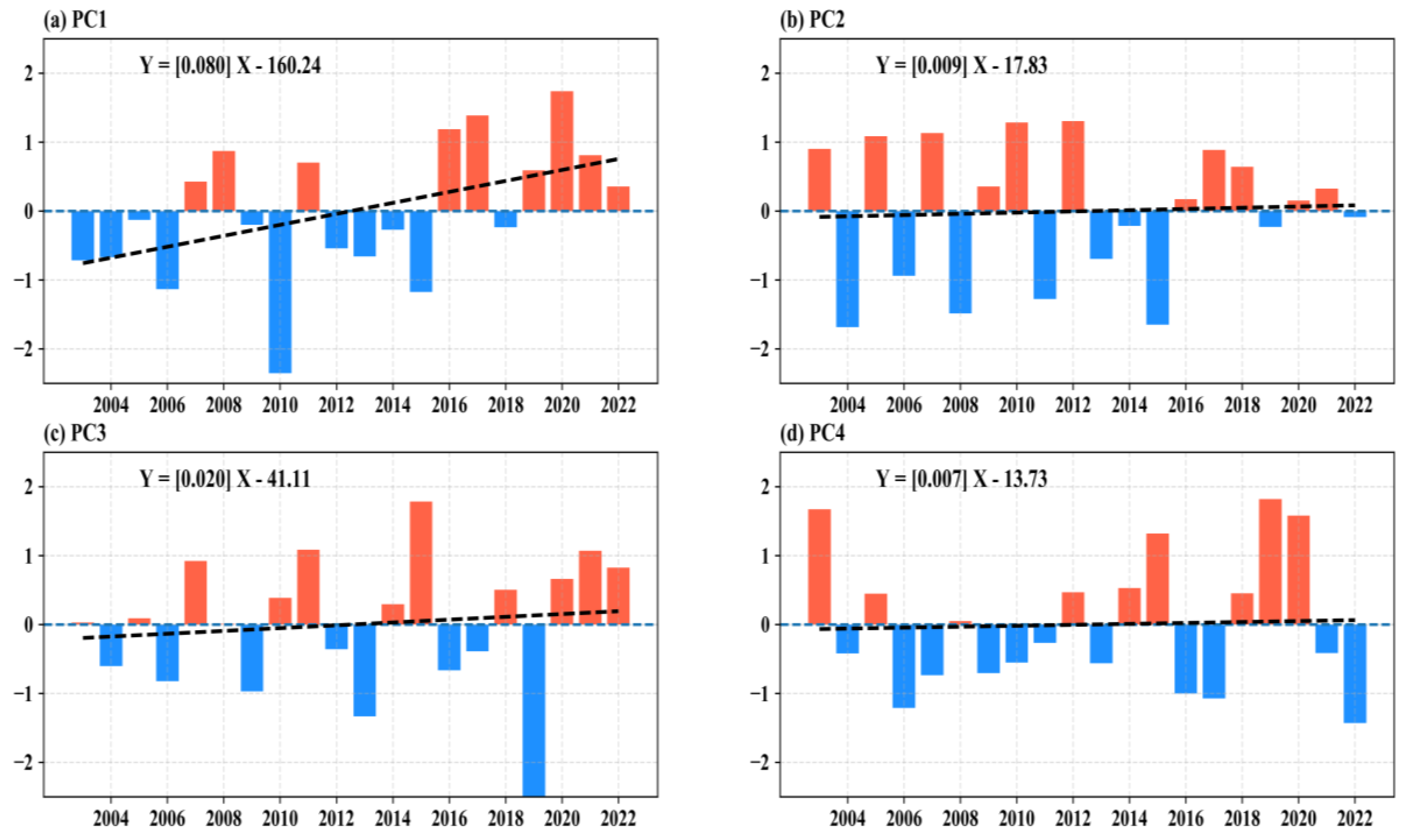
Firstly, anomaly processing was performed on China’s regional TCO data from 2003 to 2022, and then EOF analysis was performed on the TCO dataset to obtain eigenvectors and time coefficients. The larger the variance contribution rate of the eigenvector obtained from EOF decomposition, the better the mode could reflect the characteristics of the data in the space–time distribution. According to the characteristics of the EOF analysis method, generally, the variance contribution rate of the first few modes will be relatively high. As shown in Table 2 below, the variance contribution rates of the first four modes were 52.85%, 15.93%, 10.71%, and 6.05%; that is, the cumulative variance contribution rate of the first four modes was as high as 85.54%, indicating that the analysis results of the first four models using EOF in this paper were able to reflect the spatial and temporal distribution characteristics of the TCO in China to a considerable extent. At the same time, the decomposed time coefficient was used as the weight of the eigenvector, and its physical meaning contributed to the spatial features at different times. A positive value of the time coefficient represented the same trend as the spatial mode; a negative value represented the opposite trend. The results of the EOF analysis are presented in the eigenvector distribution and time coefficient graphs, where the eigenvectors have two states: “+” and “−”. The “±” distribution of the eigenvectors combined with the positive and negative values of the time coefficients for the corresponding years can be used to analyze the trend changes of the total ozone column. The specific decomposition principle of the EOF method is very complex and will not be discussed specifically here; for details, refer to reference [31].
It can be observed from Table 2 that the variance contribution rate of the first mode of EOF decomposition was the highest, as high as 52.85%, indicating that the TCO in China had good convergence. As shown in Figure 10a, the spatial distribution of the first-mode eigenvectors presented “-”, indicating that the changes in the TCO in the entire Chinese region over the past 20 years had very high consistency, and the absolute value of the change in the northeastern region was relatively large, indicating that this region belongs to a region with large fluctuations. The PC values in Figure 11a showed an increasing trend after using linear regression analysis for the period 2003 to 2022. Combined with the modal characteristics in Figure 10a, it can be shown that the overall trend of the TCO in China in recent years has been declining.
Observing Figure 10b, the second mode of the EOF decomposition, the variance contribution reaches 15.93%. The spatial distribution of eigenvectors has two different distributions in China. The total amount of ozone column in China has two opposite modes, showing a “-” distribution in parts of Northern Heilongjiang, Southern Shaanxi, Southeastern Qinghai Province, Southeastern Tibetan Province, the Yunnan and Guizhou regions, the Sichuan and Chongqing regions, and Southern China and a “+” distribution in other regions. Observing Figure 11b, the time coefficient also shows an upward trend in a slower manner over the past 20 years as a whole, and, combined with Figure 10b, we can observe that the TCO in Northern Heilongjiang, Southern Shaanxi, Southeastern Qinghai Province, Southeastern Tibetan Province, the Yunnan and Guizhou regions, the Sichuan and Chongqing regions, and Southern China shows a decreasing trend over the past 20 years, while the rest of the regions show an increasing trend.
Next, examining the third mode of EOF decomposition, observing Figure 10c, we can observe that Northeastern China and the Northwestern Xinjiang region show a “-” distribution, and the rest of the regions show a “+” distribution. Combined with Figure 11c, the time coefficient graph, the time coefficient over the last 20 years shows an overall increasing trend; thus, the overall trend of Northeastern China and the Northwestern Xinjiang region is decreasing and that for the rest of the regions is growing. The contribution rate of the fourth mode was only 6.05%, which theoretically is a low reference value, and will not be elaborated upon here.

3.3. Analysis of Factors Influencing the Change in TCO in China

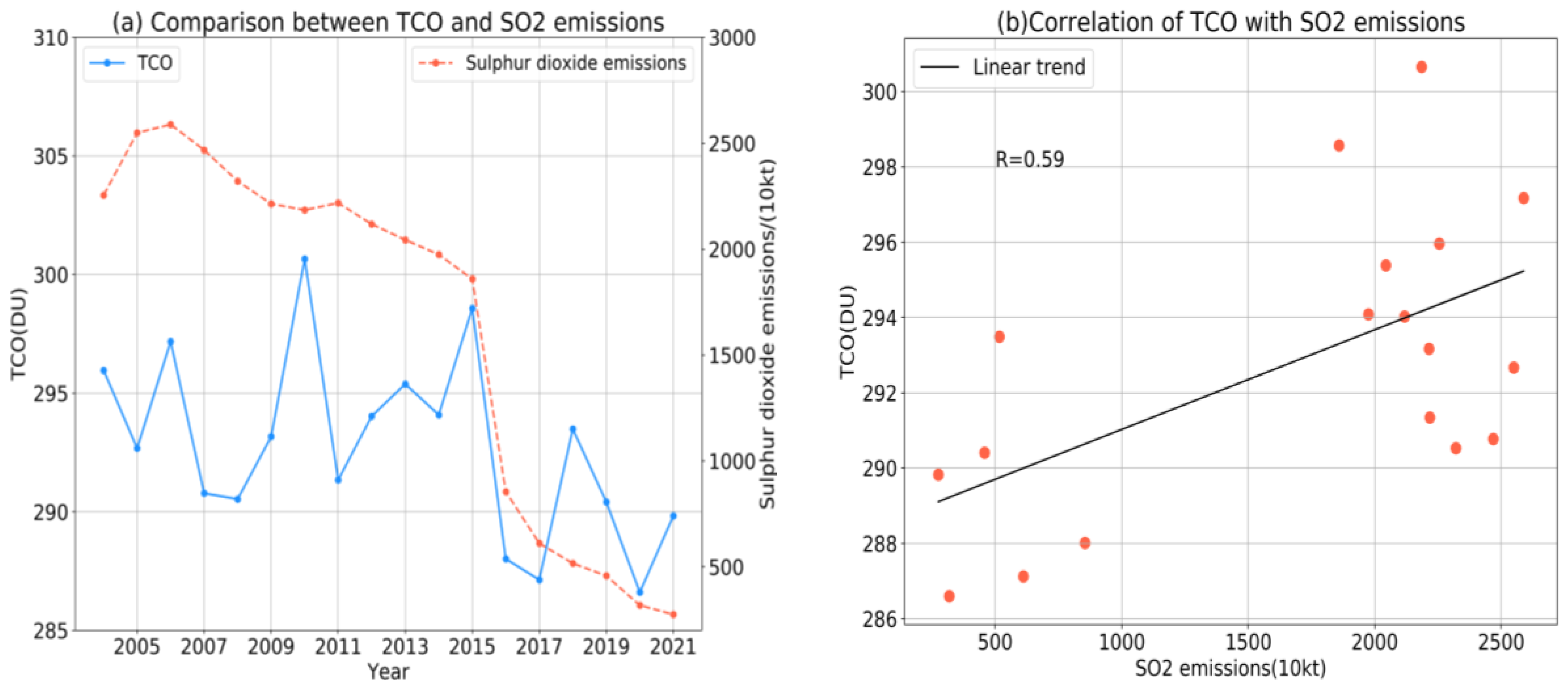
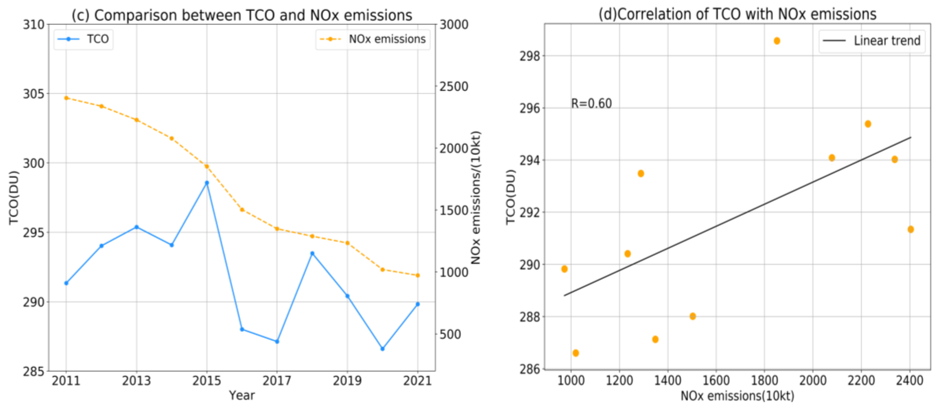
In this study, the year-by-year comparison and correlation analysis of the annual average of the TCO in China and the annual average emissions of SO2 and NOx from exhaust emissions were used. As shown in Figure 12, the correlation coefficient for the TCO and sulfur dioxide emissions reached 0.59, and the correlation coefficient for nitrogen oxide emissions reached 0.60.
NOx is one of the precursors of ozone, producing ozone after certain photochemical reactions, thereby increasing ozone levels. Increases in tropospheric ozone are likely due to increases in ozone precursors [32]. As for the possible reasons for the effect of SO2 on ozone, a review of relevant information shows that SO2 reacts chemically with oxygen atoms to produce sulfur trioxide, which leads to the oxidation of NO into precursors that are useful for ozone accumulation.

3.4. Prediction of TCO in China Based on the SARIMA Model

Firstly, the TCO data for the time series (September 2002–February 2023) of the Chinese region are visualized in this paper. In the first step, this paper tested the stationarity of the data because the SARIMA model requires that the input data must be stationary data. In this paper, the ADF test was used to test the stationarity of the data. We found that p-value = 0.00148 < 0.05 after the test; that is, the null hypothesis of the existence of a unit root was rejected, indicating that the data were already stationary. Therefore, it was only necessary to remove seasonality from the data in the next step. Therefore, seasonal differencing was used in this paper (the lag time sequence of seasonal differencing was 12 because the length of the seasonal characteristic period of the data in this paper was 12 months).
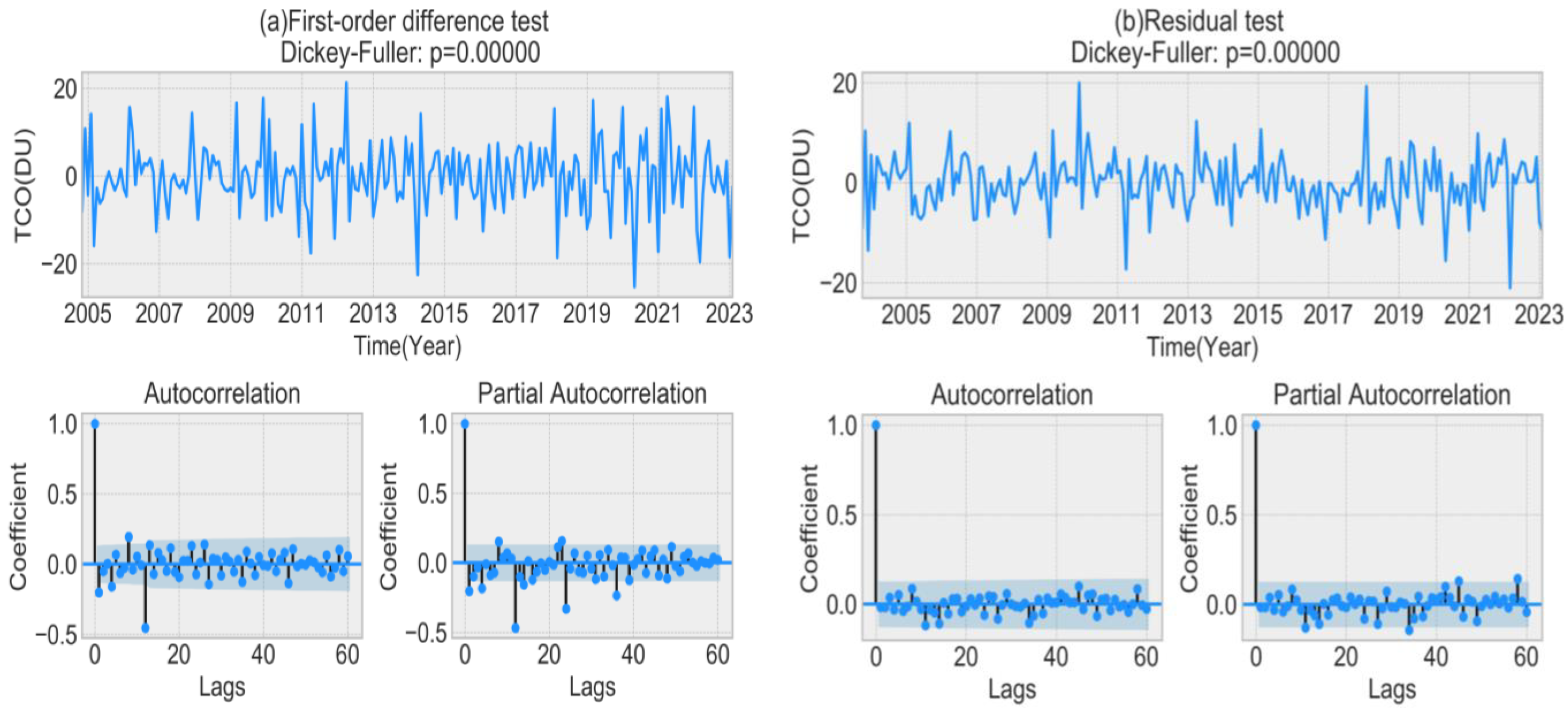
Observing the timing diagram after seasonal differencing in Figure 13b, we found that the seasonality of the data had been eliminated, but there were still a considerable number of ACF and PACF values outside the shaded area in the autocorrelation and the partial autocorrelation graphs. In this paper, this was eliminated by first-order differencing.
Examining Figure 14a, the ACF and PACF values are almost all in the shaded area. Thus, the data could be used for modeling. First of all, the seven parameters of the SARIMA model needed to be determined before training. The parameters were divided into two parts, including non-seasonal (p,d,q) and seasonal (P,D,Q,s) parameters. p is the maximum lag value of the autoregression model (AR), q is the lag value in the moving average model (MA), d refers to the non-seasonal difference number required for data processing in the model, and s refers to the seasonal cycle length of the sequence. D refers to the seasonal difference order, which can be 1 or 0, where 1 indicates whether seasonal difference processing was adopted for the data and 0 indicates that no seasonal difference was adopted.
First, s = 12, because the seasonal cycle is a 12-month cycle. D = 1 because a seasonal difference was observed, and d = 1 because a first-order difference was observed. The next step was to determine the parameters of p, q, P, and Q. This paper determined the non-seasonal parameters p and q by observing the autocorrelation function (ACF) and partial autocorrelation function (PACF) graphs of Figure 14a. ACF is a complete autocorrelation function that provides us with the autocorrelation value of any series with lagged values. In simple terms, it describes the degree of correlation between the current value of the series and its past values. PACF is a partial autocorrelation function. Instead of finding the correlation between a lag such as the ACF and the current one, it finds the correlation between the residuals (which remain after removing the effects already explained by the previous lag) and the next lag value. q may be 1 because it can be observed from the ACF graph of Figure 14a that it is a first-order truncation because, after the first-order lag, almost 95% of the autocorrelation coefficients fall within the range of two standard deviations. p may be 1 because it is also after the first order that the partial correlation coefficient graph appears to be trailing. For the seasonal parameters P and Q, the method was similar, except that the peak corresponding to the lag point at the position of the multiple of the seasonal period is observed. First, it is possible that Q is 1 because the peak at the 12th lag point in the ACF diagram of Figure 14a is relatively clear. P may be 1 because the 12th lag point is also clear in the PACF diagram of Figure 14a. However, in the final analysis, determining parameters by examining auto- and partial correlation graphs is still somewhat subjective, but that is not to say that they are meaningless because the ranges of p, q, P, and Q could be roughly determined by observation; on this basis, iterating the values around these parameters through Python programs reduced part of the computation. Finally, each group of parameters was compared using AIC information criterion to determine the best parameter.
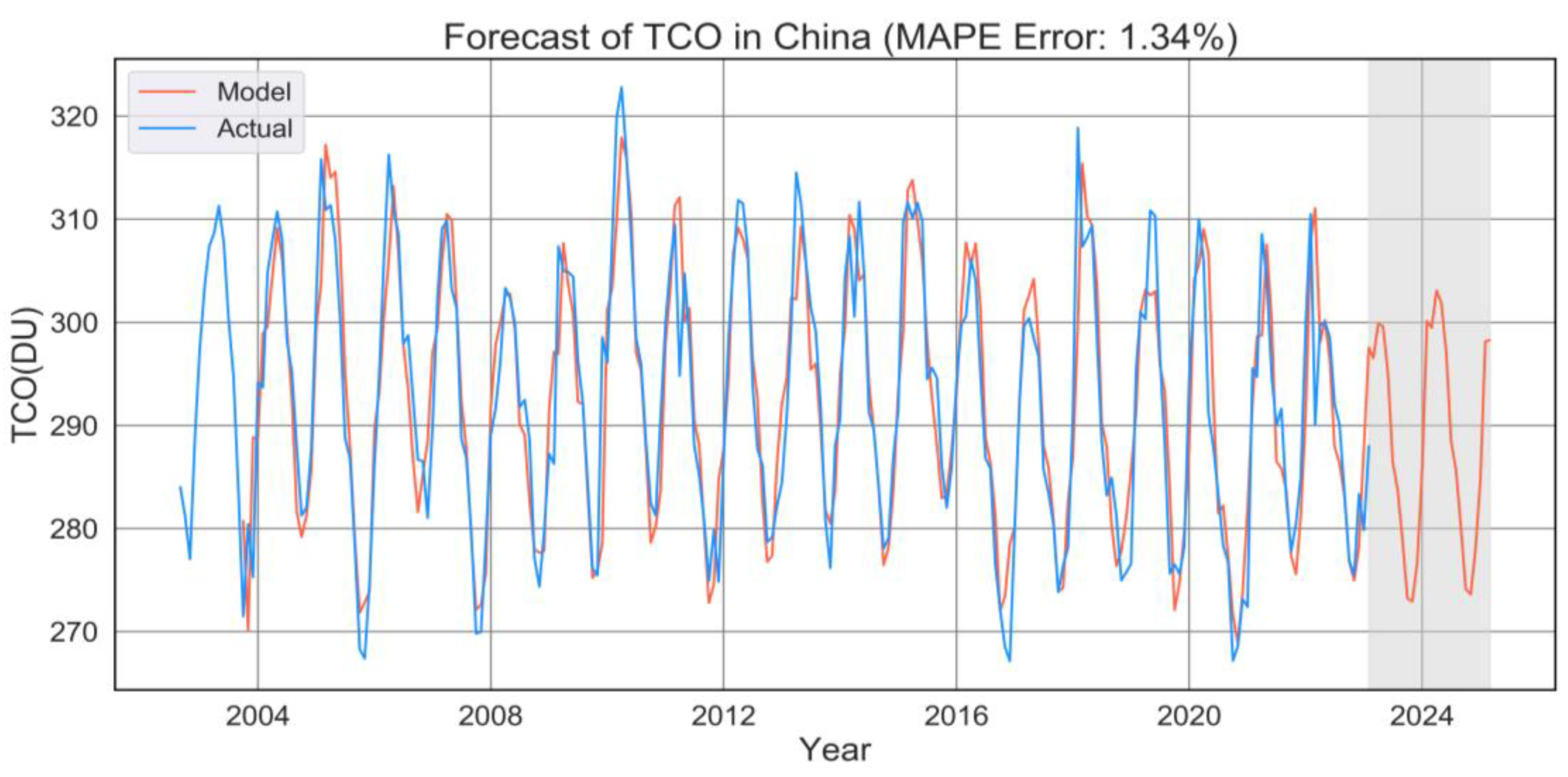
After comparing multiple sets of values of AIC information criterion, the parameters finally determined were SARIMA (1, 1, 2) × (0, 1, 2, 12). After model fitting, this paper conducted a residual test on the SARIMA model, as shown in Figure 14b. Through auto- and partial correlation graphs, it was found that almost all correlation coefficients fell within a 95% confidence interval, which indicated that the model had a very good degree of fitting. Finally, after the parameters had been determined, they were inputted to train the SARIMA model, and the trained model was used for prediction. As shown in Figure 15, the TCO in China was predicted by the SARIMA model. The blue curve is the time series curve drawn from the real value of the TCO, while the red curve is drawn from the predicted value obtained using the SARIMA model.
By comparing the red and blue curves in Figure 15, it can be observed that the fitted curve value within the existing time data had a relatively high coincidence degree with the actual value curve, which also illustrates that the model trained in this paper, from an intuitive point of view, had good precision. However, it is still a little subjective to simply observe that two curves fit well. Therefore, in order to verify the accuracy of the previous judgment, MAPE (mean absolute percentage error), one of the evaluation indexes of the model, was introduced in this paper to determine fitting errors and measure the accuracy of the model. According to the calculation of the MAPE evaluation index, the MAPE value of this algorithm model was as low as 1.34%, which indicated that the accuracy of this algorithm model fitting was very high.

4. Discussion

Based on data collected by AIRS (September 2002 to February 2023), the temporal, frequency, and spatial distribution of TCO over China in the last 22 years was studied by linear regression and coefficient of variation methods. After data processing and analysis, it was found that the variation curve of multi-year monthly average TCO was similar to a “sine” curve, which is consistent with the research conclusions of Zhang, J.Q. et al. [7] on the monthly mean of TCO in North China. It was found that the TCO in spring was the highest in all four seasons, and its annual average rate of decline was also the highest in spring. Traditionally, research in the field of meteorology tends to focus on the analysis of spatial and temporal variability characteristics; however, in recent years, Fourier transform, wavelet transform, and other frequency domain analysis tools have been introduced into the field of meteorological research. Szolgayova, E. et al. [33] studied the long-term variability of the Danube River flow and its relation to precipitation and air temperature using wavelet transforms, cross wavelets, and other methods. Ma, L.H. et al. [34] used continuous wavelet and cross wavelet transform to investigate the influence of the 11-year solar cycle on precipitation in Huashan Mountain, China, over the last 300 years. As there are few studies on the frequency domain characteristic changes of the TCO in China in recent years, that is, the analysis of the periodic characteristics of the TCO in China in the last 22 years, this study introduced wavelet analysis to analyze the TCO in the frequency domain and found that there is indeed a phenomenon of multiple groups of cycles nested, with main cycles of 14 and 6 years. It was also found that the corresponding periods under the two main cycles were different, thus illustrating the advantages of wavelet analysis in the field of time-frequency analysis.
The spatial distribution of annual TCO in China was also studied in this paper. We found that the TCO in Northeast China was the highest from 2003 to 2022, while the total ozone in South China, Qinghai-Tibet Plateau, and Southwest China was lower. In this study, EOF analysis was also used to study the mode of TCO in China and it was found that the contribution rate of the first mode was as high as 52.85%. Some studies that also used EOF for spatiotemporal analysis were also referred to. For example, Gao, W. et al. [35] used EOF analysis to study the spring SST anomalies in the South China Sea and its adjacent waters. The first mode contribution rate was as high as 45.15%. Generally speaking, when the contribution rate of the first mode in EOF analysis is relatively large, the mode has a high reference value.

5. Conclusions

Based on the dataset of the TCO in China (September 2002 to February 2023), this paper analyzed and studied the TCO in China over the last 22 years. Combined with the analysis of the full text, we come to the following conclusions:
(1)
Firstly, the monthly average data of AIRS were selected for correlation analysis with the data of the BLD, BRW, and OHP stations in the same period, and the Pearson correlation coefficients were 0.9509, 0.9771, and 0.9403, respectively. The above verification showed that the AIRS data used in this study were reliable.
(2)
The annual mean data of the TCO in China from 2003 to 2022 were analyzed. The TCO in 2010 was the highest of that in the past 20 years, reaching 300.7 DU. In 2020, the TCO reached 286.6 DU, the lowest level in nearly 20 years. The overall trend from 2003 to 2022 was found to be a slow decline by linear regression analysis, with a change rate of K = −0.29 DU/a. From the results of the coefficient of variation, the annual fluctuation of the TCO in 2005 was the greatest and that in 2008 was the smallest. Analysis using an M-K mutation test found that TCO experienced a mutation around 2016.
(3)
The multi-year monthly mean TCO from 2003 to 2022 was analyzed. In these 20 years, the average TCO was highest in April and lowest in November each year. At the same time, using the coefficient of variation to analyze the fluctuation of the multi-year monthly mean TCO, it was found that the month with the largest fluctuation in the total ozone column was February and the most stable month was July. From a seasonal perspective, the fluctuation in TCO change was the smallest in autumn and the largest in winter. The order of the fluctuation degree of TCO change in the four seasons was winter > spring > summer > autumn.
(4)
The multi-annual mean value of the four seasons in 2003 to 2022 was analyzed. In terms of quantity, TCO levels in spring were the highest, while TCO levels in autumn were the lowest. The order of total column ozone size in the four seasons was spring > summer > winter > autumn. From the perspective of change rate, the decline rate was the fastest in summer and the slowest in winter. The order of decline rate in the four seasons was spring > summer > winter > autumn.
(5)
Wavelet transform was used to analyze the frequency domain characteristics of TCO over China from 2003 to 2022. The study revealed that there were two major time scales, known as major cycles. Among them, 14 years was the first main cycle corresponding to the change cycle of the TCO in China for approximately 10 years, with 2003~2022 experiencing two cycles; 6 years was the change cycle corresponding to the second main cycle for approximately 4 years, with 2003~2022 experiencing approximately five cycles. The above analysis results fully demonstrate that the cyclical characteristics of the TCO in China are very complex and various.
(6)
The spatial distribution characteristics of China’s TCO are extremely clear, with clear latitude and longitude distribution characteristics. First, as the latitude increased, the TCO also increased. Generally speaking, the TCO in Northeast China and Northern China was relatively high; the TCO in Southwestern China, Qinghai-Tibet Plateau, and Southern China was relatively low. The multi-year average time series comparison of the TCO in China divided into seven major regions found that in the 20 years from 2003 to 2022, their order of size was as follows: Northeastern China > Northern China > Northwestern China > Central and Eastern China > Qinghai-Tibet Plateau > Southwestern China > Southern China. Using EOF analysis to decompose the space–time mode of the TCO in China, the variance contribution rate of the first mode was as high as 52.85%, which had the highest reference value among many modes. The cumulative contribution rate of the first four modes reached 85.54%. Among them, the spatial distribution of the first mode presented “-”, indicating that the changes in the TCO in the entire Chinese region in the past 20 years had a very high consistency.
(7)
Using the correlation analysis of the TCO and SO2 emissions and NOx emissions, it was found that changes in the total amount of ozone are related to these factors. The correlation coefficient for the TCO and sulfur dioxide emissions reached 0.59 and the correlation coefficient for nitrogen oxide emission reached 0.60.
(8)
This study used the SARIMA model to predict the TCO of China. Considering the seasonality and other characteristics of the data, the data were pre-processed and then trained with the AIC information criterion to find the best model parameters. The best prediction model of monthly average TCO in China was determined to be SARIMA (1, 1, 2) × (0, 1, 2, 12); we used this model to forecast the TCO over China for the next 24 months. In order to objectively measure the accuracy of the prediction results, MAPE was introduced to calculate the error rate, and the error rate of the model prediction was as low as 1.34%, which shows that the model fitted in this study had good accuracy. This result indicates that the predicted TCO trend of China was also relatively accurate.
This study was a systematic study and elaboration of the change characteristics of the TCO in China from multiple perspectives; we hope that these results can provide a certain reference for future research related to TCO. Finally, due to the complex and diverse characteristics of China’s terrain, landform, and climatic conditions and limited data, this study only engaged in a preliminary elaboration and discussion of the characteristics and causes of change; further in-depth research is needed in the future.

Author Contributions

C.T.: methodology, writing—review and editing. F.Z. (Fangzheng Zhu): methodology and writing—original draft. Y.W.: Software, investigation, and resources. X.T.: investigation and resources. J.Y.: investigation and validation. F.Z. (Fengmei Zhao): investigation and validation. All authors have read and agreed to the published version of the manuscript.

Funding

This study was supported by the Graduate Innovation Foundation of Anhui University of Science and Technology (no. 2022CX2087), the Graduate Student Academic Innovation Project of Anhui Province of China (no. 2022xscx076), and the University Natural Science Research Project of Anhui Province of China (no. 2022AH050083K; J2019A0103).

Institutional Review Board Statement

Not applicable.

Informed Consent Statement

Not applicable.

Data Availability Statement

We would like to thank the AQUA-AIRS team for providing the necessary datasets used in this study. The version 6.0 level 3 dataset of AIRS was downloaded from https://disc.gsfc.nasa.gov/datasets (accessed on 8 April 2023). We would also like to thank the NOAA team for providing the meteorological station datasets used in this study, downloaded from https://www.esrl.noaa.gov/gmd/dv/data/index.php?category=Ozone (accessed on 11 April 2023). We are also very grateful to the National Bureau of Statistics of China for providing the datasets for the correlation analysis in this study, downloaded from http://www.stats.gov.cn/ (accessed on 10 April 2023).

Acknowledgments

We sincerely thank the NASA Goddard Space Flight Center for providing the AIRS total ozone column dataset for this study, NOAA for providing the atmospheric background station total ozone column dataset, and the National Bureau of Statistics of China for providing the annual datasets of SO2 and NOx in exhaust emissions. We are grateful to the Project Supported by the Specialized Research Fund for State Key Laboratories.

Conflicts of Interest

The authors declare that there are no conflict of interest regarding the publication of this paper.

References

  1. Chen, L.; Yu, B.; Chen, Z.; Li, B.; Wu, J. Investigating the temporal and spatial variability of total ozone column in the Yangtze River Delta using satellite data: 1978–2013. Remote. Sens. 2014, 6, 12527–12543. [Google Scholar] [CrossRef]
  2. Midya, S.K.; Goswami, S. Seasonal variation of daily total column ozone (TCO) and its depletion and formation role on surface temperature over Ahmedabad (23°01′ N, 72°39′ E). Indian J. Phys. 2013, 87, 953–961. [Google Scholar] [CrossRef]
  3. Staehelin, J.; Harris, N.R.P.; Appenzeller, C.; Eberhard, J. Ozone trends: A review. Rev. Geophys. 2001, 39, 231–290. [Google Scholar] [CrossRef]
  4. Jana, P.K.; Bhattacharyya, S.; Banerjee, A. Effect of some climatic parameters on tropospheric and total ozone column over Alipore (22.52° N, 88.33° E), India. J. Earth Syst. Sci. 2014, 123, 1653–1669. [Google Scholar] [CrossRef]
  5. Shin, D.; Oh, Y.-S.; Seo, W.; Chung, C.-Y.; Koo, J.-H. Total Ozone Trends in East Asia from Long-Term Satellite and Ground Observations. Atmosphere 2021, 12, 982. [Google Scholar] [CrossRef]
  6. Wang, W.; Cheng, T.; van der A, R.J.; de Laat, J.; Williams, J.E. Verification of the Atmospheric Infrared Sounder (AIRS) and the Microwave Limb Sounder (MLS) ozone algorithms based on retrieved daytime and night-time ozone. Atmos. Meas. Tech. 2021, 14, 1673–1687. [Google Scholar] [CrossRef]
  7. Zhang, J.; Li, D.; Bian, J.; Xuan, Y.; Chen, H.; Bai, Z.; Wan, X.; Zheng, X.; Xia, X.; Lü, D. Long-term ozone variability in the vertical structure and integrated column over the North China Plain: Results based on ozonesonde and Dobson measurements during 2001–2019. Environ. Res. Lett. 2021, 16, 074053. [Google Scholar] [CrossRef]
  8. Zhou, P.; Wen, Y.; Yang, J.; Yang, L.; Liang, M.; Wen, T.; Cai, S. Spatiotemporal Variation, Driving Mechanism and Predictive Study of Total Column Ozone: A Case Study in the Yangtze River Delta Urban Agglomerations. Remote. Sens. 2022, 14, 4576. [Google Scholar] [CrossRef]
  9. Bian, J.; Yan, R.; Chen, H.; Lu, D.; Massie, S.T. Formation of the summertime ozone valley over the Tibetan Plateau: The Asian summer monsoon and air column variations. Adv. Atmos. Sci. 2011, 28, 1318–1325. [Google Scholar] [CrossRef]
  10. Zhang, J.; Tian, W.; Xie, F.; Tian, H.; Luo, J.; Zhang, J.; Liu, W.; Dhomse, S. Climate warming and decreasing total column ozone over the Tibetan Plateau during winter and spring. Tellus B Chem. Phys. Meteorol. 2014, 66, 23415. [Google Scholar] [CrossRef]
  11. Chidinma, O.E.; Yan, Y.-H.; Yin, Z.; Kingsley, O.U.; Nneka, O.F. Impact of solar and geomagnetic activities on total column ozone in China. J. Atmospheric Solar-Terrestrial Phys. 2021, 223, 105738. [Google Scholar] [CrossRef]
  12. Okoro, E.C.; Yan, Y.-H.; Bisoi, S.K.; Zhang, Y. Response and periodic variation of total atmospheric ozone to solar activity over Mountain Waliguan. Adv. Space Res. 2021, 68, 2257–2271. [Google Scholar] [CrossRef]
  13. Wang, S.; Huo, Y.; Mu, X.; Jiang, P.; Xun, S.; He, B.; Wu, W.; Liu, L.; Wang, Y. A High-Performance Convolutional Neural Network for Ground-Level Ozone Estimation in Eastern China. Remote. Sens. 2022, 14, 1640. [Google Scholar] [CrossRef]
  14. Zou, M.; Xiong, X.; Wu, Z.; Yu, C. Ozone Trends during 1979–2019 over Tibetan Plateau Derived from Satellite Observations. Front. Earth Sci. 2020, 8, 579624. [Google Scholar] [CrossRef]
  15. Valipour, M. Long-term runoff study using SARIMA and ARIMA models in the United States. Meteorol. Appl. 2015, 22, 592–598. [Google Scholar] [CrossRef]
  16. Wang, H.; Wang, Y.; Cai, K.; Zhu, S.; Zhang, X.; Chen, L. Evaluating the Performance of Ozone Products Derived from CrIS/NOAA20, AIRS/Aqua and ERA5 Reanalysis in the Polar Regions in 2020 Using Ground-Based Observations. Remote. Sens. 2021, 13, 4375. [Google Scholar] [CrossRef]
  17. Liu, J.; Hagan, D.F.T.; Liu, Y. Global Land Surface Temperature Change (2003–2017) and Its Relationship with Climate Drivers: AIRS, MODIS, and ERA5-Land Based Analysis. Remote. Sens. 2020, 13, 44. [Google Scholar] [CrossRef]
  18. Wu, J.; Chen, X.; Chang, T.-J. Correlations between hydrological drought and climate indices with respect to the impact of a large reservoir. Theor. Appl. Clim. 2019, 139, 727–739. [Google Scholar] [CrossRef]
  19. Kamau-Muthoni, F.; Omondi-Odongo, V.; Ochieng, J.; Mugalavai, E.M.; Kjumula-Mourice, S.; Hoesche-Zeledon, I.; Mwila, M.; Bekunda, M. Long-term spatial-temporal trends and variability of rainfall over eastern and Southern Africa. Theor. Appl. Climatol. 2019, 137, 1869–1882. [Google Scholar] [CrossRef]
  20. Gargour, C.; Gabrea, M.; Ramachandran, V.; Lina, J.-M. A short introduction to wavelets and their applications. IEEE Circuits Syst. Mag. 2009, 9, 57–68. [Google Scholar] [CrossRef]
  21. Tuo, W.; Zhang, X.; Song, C.; Hu, D.; Liang, T. Annual precipitation analysis and Forecasting—Taking Zhengzhou as an example. Water Supply 2020, 20, 1604–1616. [Google Scholar] [CrossRef]
  22. Zhang, M.-L.; Liu, C.; Wan, W.; Liu, L.; Ning, B. A global model of the ionospheric F2 peak height based on EOF analysis. Ann. Geophys. 2009, 27, 3203–3212. [Google Scholar] [CrossRef]
  23. Yu, Y.; Wan, W.; Xiong, B.; Ren, Z.; Zhao, B.; Zhang, Y.; Ning, B.; Liu, L. Modeling Chinese ionospheric layer parameters based on EOF analysis. Space Weather. 2015, 13, 339–355. [Google Scholar] [CrossRef]
  24. Mushtaq, R. Augmented dickey fuller test. SSRN J. 2011. [CrossRef]
  25. Portet, S. A primer on model selection using the Akaike Information Criterion. Infect. Dis. Model. 2020, 5, 111–128. [Google Scholar] [CrossRef] [PubMed]
  26. Butchart, N. The Brewer-Dobson circulation. Rev. Geophys. 2014, 52, 157–184. [Google Scholar] [CrossRef]
  27. Chen, D.; Nunez, M. Temporal and spatial variability of total ozone in Southwest Sweden revealed by two ground-based instruments. Int. J. Climatol. A J. R. Meteorol. Soc. 1998, 18, 1237–1246. [Google Scholar] [CrossRef]
  28. Tung, K.K.; Yang, H. Dynamic variability of column ozone. J. Geophys. Res. Atmos. 1988, 93, 11123. [Google Scholar] [CrossRef]
  29. Antón, M.; Bortoli, D.; Costa, M.J.; Kulkarni, P.; Domingues, A.; Barriopedro, D.; Serrano, A.; Silva, A.M. Temporal and spatial variabilities of total ozone column over Portugal. Remote. Sens. Environ. 2011, 115, 855–863. [Google Scholar] [CrossRef]
  30. Aesawy, A.M.; Mayhoub, A.B.; Sharobim, W.M. Seasonal variation of photochemical and dynamical components of ozone in subtropical regions. Theor. Appl. Clim. 1994, 49, 241–247. [Google Scholar] [CrossRef]
  31. Tian, X.; Tang, C.; Wu, X.; Yang, J.; Zhao, F.; Liu, D. The global spatial-temporal distribution and EOF analysis of AOD based on MODIS data during 2003–2021. Atmos. Environ. 2023, 302, 119722. [Google Scholar] [CrossRef]
  32. Liu, J.; Strode, S.A.; Liang, Q.; Oman, L.D.; Colarco, P.R.; Fleming, E.L.; Manyin, M.E.; Douglass, A.R.; Ziemke, J.R.; Lamsal, L.N.; et al. Change in Tropospheric Ozone in the Recent Decades and Its Contribution to Global Total Ozone. J. Geophys. Res. Atmos. 2022, 127, e2022JD037170. [Google Scholar] [CrossRef]
  33. Szolgayova, E.; Parajka, J.; Blöschl, G.; Bucher, C. Long term variability of the Danube River flow and its relation to precipitation and air temperature. J. Hydrol. 2014, 519, 871–880. [Google Scholar] [CrossRef]
  34. Ma, L.H.; Han, Y.B.; Yin, Z.Q. Possible Influence of the 11-year Solar Cycle on Precipitation in Huashan Mountain of China over the Last 300 Years. Earth Moon Planets 2010, 107, 219–224. [Google Scholar] [CrossRef]
  35. Gao, W.; Yang, S.; Hu, X.; Wei, W.; Xiao, Y. Characteristics and Formation Mechanisms of Spring SST Anomalies in the South China Sea and Its Adjacent Regions. Atmosphere 2019, 10, 649. [Google Scholar] [CrossRef]
Figure 1. Month-to-month comparison and correlation analysis between AIRS data and atmospheric background station data. (a,d) BLD. (b,e) BRW. (c,f) OHP.
Atmosphere 14 00941 g001aAtmosphere 14 00941 g001b
Figure 2. Interannual variation trend. (a) Analysis of the annual mean change in the TCO over China. (b) Annual mean map of M-K mutation test.
Atmosphere 14 00941 g002
Figure 3. (a) Monthly time series analysis of TCO over China. (b) Comparison of multi-year monthly mean TCO over China.
Atmosphere 14 00941 g003
Figure 4. Analysis of different seasonal averages of TCO over China from 2003 to 2022. (a) Spring. (b) Summer. (c) Autumn. (d) Winter.
Atmosphere 14 00941 g004
Figure 5. Wavelet analysis of TCO over China from 2003 to 2022. (a) Wavelet real part. (b) Wavelet square difference curve. (c) Wavelet modulus. (d) Wavelet modulus square.
Atmosphere 14 00941 g005
Figure 6. Main cycles analysis. (a) The first main cycle. (b) The second main cycle.
Atmosphere 14 00941 g006
Figure 7. (a) Spatial distribution of TCO in China. (b) Comparative analysis of seven regional time series.
Atmosphere 14 00941 g007
Figure 8. Spatial distribution of annual four-season mean TCO over China. (a) Spring. (b) Summer. (c) Autumn. (d) Winter.
Atmosphere 14 00941 g008
Figure 9. Latitude and longitude distribution of TCO in China. (a) Latitude. (b) Longitude.
Atmosphere 14 00941 g009
Figure 10. Spatial distribution of EOF of the TCO over China. (a) First mode. (b) Second mode. (c) Third mode. (d) Fourth mode.
Atmosphere 14 00941 g010
Figure 11. PC values corresponding to the four modes of EOF decomposition. (a) PC values of the first mode. (b) PC values of the second mode. (c) PC values of the third mode. (d) PC values of the fourth mode.
Atmosphere 14 00941 g011
Figure 12. (a) Comparison of TCO and SO2 emissions. (b) Correlation analysis of TCO and SO2 emissions. (c) Comparison of TCO and NOx emissions. (d) Correlation analysis of TCO and NOx emissions.
Atmosphere 14 00941 g012aAtmosphere 14 00941 g012b
Figure 13. (a) Time series and auto- and bias correlation graphs. (b) Seasonal difference and auto- and bias correlation graphs.
Atmosphere 14 00941 g013
Figure 14. (a) First-order difference and auto- and bias correlation graphs. (b) Residual test and auto-and bias correlation graphs.
Atmosphere 14 00941 g014
Figure 15. Prediction of TCO over China based on the SARIMA model.
Atmosphere 14 00941 g015
Table 1. Site information.
SiteNationLatitudeLongitude
BLDUnited States39.9° N105.3° W
BRWUnited States71.3° N156.6° W
OHPFrance43.9° N6.8° E
Table 2. The variance contribution rate of EOF.
Mode1234
Variance contribution rate52.85%15.93%10.71%6.05%
Cumulative variance contribution rate52.85%68.78%79.49%85.54%
Disclaimer/Publisher’s Note: The statements, opinions and data contained in all publications are solely those of the individual author(s) and contributor(s) and not of MDPI and/or the editor(s). MDPI and/or the editor(s) disclaim responsibility for any injury to people or property resulting from any ideas, methods, instructions or products referred to in the content.