Article

Examining the Effectiveness of Doppler Lidar-Based Observation Nudging in WRF Simulation for Wind Field: A Case Study over Osaka, Japan

Research and Development Center, Japan Meteorological Corporation, Osaka 530-0011, Japan
*
Author to whom correspondence should be addressed.
Atmosphere 2023, 14(6), 972; https://doi.org/10.3390/atmos14060972
Submission received: 3 May 2023 / Revised: 19 May 2023 / Accepted: 30 May 2023 / Published: 2 June 2023
(This article belongs to the Section Atmospheric Techniques, Instruments, and Modeling)

Abstract

:
This study attempts to improve the accuracy of wind field simulations in the Weather Research and Forecasting (WRF) model by incorporating Doppler lidar-based wind observations over the Osaka region of Japan. To achieve this, a Doppler lidar was deployed in Osaka city, and multi-layer wind measurements were obtained for one month (August 2022). These measurements were then assimilated into the WRF model using the observation nudging technique. Two simulations were conducted: one with nudging disabled, and the other with nudging enabled with data assimilation, while keeping all other configurations constant. The results were evaluated by comparing the simulations with the lidar observation at the lidar location where the wind data were nudged during the simulation, as well as with the AMeDAS station observations at other locations far from the lidar. The results indicated that not only the wind field, but other weather variables such as temperature, were better captured in the simulation using lidar-based nudging compared to the simulation without nudging.

1. Introduction

The Weather Research and Forecasting (WRF) model is a state-of-the-art atmospheric modeling system that is widely used for atmospheric research and operational forecasting applications. It is a mesoscale numerical weather prediction model that can simulate various meteorological phenomena such as wind, temperature, precipitation and other atmospheric variables with high spatial and temporal resolutions [1]. WRF has been used in various atmospheric research studies, including the analysis of severe weather events, air quality modeling, climate change projections, and renewable energy assessments [2,3,4,5,6,7,8,9,10,11,12].
WRF offers multiple options for simulating atmospheric processes at high spatial and temporal resolutions by selecting the appropriate domain, input, physics, and dynamics. However, due to the complexity of the atmosphere, choosing the appropriate model configuration for a specific region or application is crucial in order to obtain accurate results. Therefore, many studies have been conducted to evaluate the sensitivity of the WRF model to different model configurations over the target region to find a suitable model setup with a higher accuracy [13,14,15,16,17,18].
Li et al. [19] recently conducted a sensitivity study using the WRF model to investigate the offshore wind profile over the Baltic Sea. The study examined the impact of different forcing datasets on the model’s ability to reproduce accurate wind profiles. The results showed that the selection of the forcing data played a critical role in improving the model’s accuracy in reproducing the wind profile. This finding suggests that improving the initial and boundary conditions can lead to better model performance in reproducing atmospheric processes. The importance of choosing appropriate initial and boundary conditions for the WRF model has been emphasized in several studies [14,20,21,22].
Considering the improvements in the model inputs, four-dimensional data assimilation techniques, such as variational methods [23,24,25,26,27] and nudging methods [28,29,30,31,32,33], are commonly used in the WRF simulation. The nudging method involves merging the model simulations toward some observations continuously, which ensures that the simulations do not deviate from the observed data [34,35]. One of the advantages of nudging methods is that they can incorporate various observations, including in situ and remote sensing measurements. Observation nudging has been widely used in atmospheric modeling for different purposes, such as modeling the path of tropical cyclones [23,36], the early warning of extreme weather events [31,32,37], improving air quality modeling [38], and wind energy-related studies [39].
The observations used in the assimilation process mainly come from satellites, radiosondes, and Doppler lidar measurements [14,23,39,40]. However, satellite observations lack data on the multilayer wind profile when a Doppler lidar is not available, and radiosondes launched at different times do not provide sufficiently time-resolved data for the wind profile. In contrast, the Doppler lidar emits laser light into the sky and receives scattered light from aerosols, such as invisible dust and fine particles. By measuring the dynamic velocity of the aerosols from the Doppler frequency shift of the scattered light, the Doppler lidar can calculate the wind direction and speed every few seconds. Therefore, Doppler lidar-based wind measurements are expected to provide an accurate time-resolved wind profile.
In this study, we examined the accuracy of the wind profile in the WRF model simulation over Osaka, Japan. The study involved the installation of a Doppler lidar in Osaka city, data collection for about a month (August, 2022) as a case study, and the use of the Doppler lidar-based observation nudging method over the region. The primary objective of the study was to determine whether assimilating the lidar-based observed data into the model input could produce a more accurate wind profile. By analyzing the wind profile accuracy in the WRF model simulation over the Osaka region of Japan, the study aimed to provide valuable insights into the potential use of Doppler lidar and ways to improve the accuracy of wind profile predictions for future applications.

2. Methods and Data

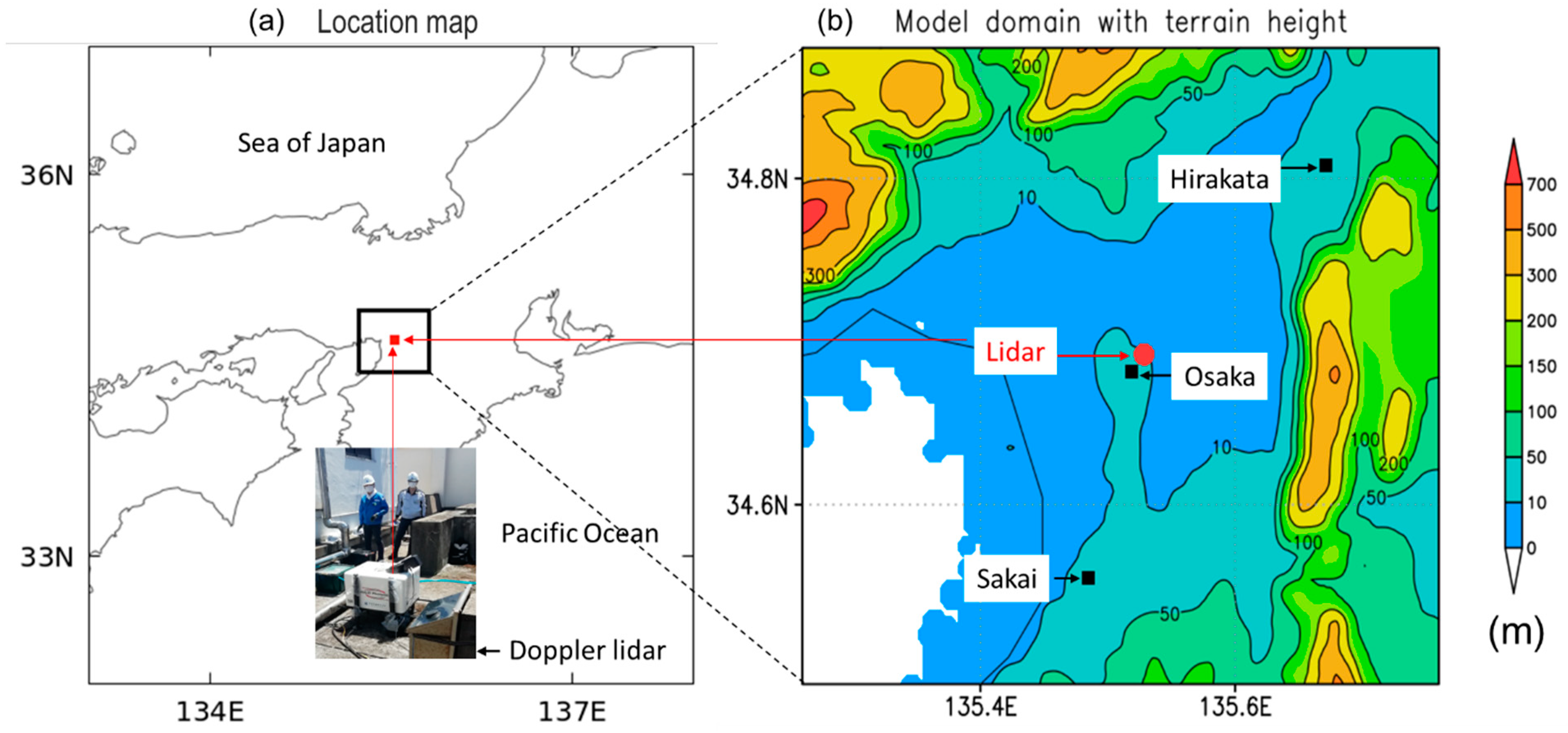
2.1. Study Region and the Doppler Lidar Setup

The present study focuses on the Osaka region (Figure 1), a city situated along the Pacific coast in western Japan. The coastal areas in and around Osaka are predominantly flat and overlook the Seto Inland Sea. The reason behind selecting this particular region for the study is that Osaka and the Seto Inland Sea are enclosed by mountains, resulting in weaker winds in comparison to regions facing expansive oceans such as the Japan Sea and the Pacific. Additionally, the surface conditions in Osaka are complex due to the mixture of urban–rural areas and land–water interfaces, requiring vertical wind profiling.
However, the paucity of observation data over water bodies, combined with the inaccuracy and low resolution of heat conditions over urban areas, make numerical simulations unreliable. To address this, we installed a Doppler lidar (StreamLine PRO, HALO Photonics, Worcestershire, UK) in Osaka city at a specific location, 34.6631 N, 135.5287 E (marked in red square in Figure 1), to obtain horizontal and vertical wind speeds and wind directions from the laser beams directed skyward in different directions. We collected the instantaneous wind profiles at 100 different heights above the ground level ranging from 14 m to 2839 m at approximately 30 s intervals for about one month (August 2022) using the Vertical Profiling Lidar device (VL) mounted in the Velocity Azimuth Display (VAD) mode of the Doppler lidar. The data availability of the Doppler lidar can vary depending on the specific instrument used and the atmospheric conditions. It is worth noting that the data availability may decrease in certain weather conditions, such as rain, fog, or low clouds. These atmospheric conditions can affect the lidar’s ability to accurately measure wind velocity and direction due to signal attenuation, scattering, and other factors. Typically, most modern Doppler lidar systems can provide reliable wind measurements with a high accuracy of about 0.1 m s–1 at a 1000 m altitude range. To ensure the quality of the data, we processed the data by taking the mean at 10 min intervals.

2.2. Model Configuration and Experimental Design

The Advanced Research WRF model version 3.9.1.1 [1] was set up over the designated area of interest (135.23–135.82 E and 34.45–34.93 N) with a 500 m horizontal grid resolution. The center of the model domain was placed at the location of the Doppler lidar, as shown in Figure 1. The model configuration consisted of 40 vertical levels and a 100 × 100 horizontal grid points. The physics schemes incorporated into the model included the Mellor–Yamada–Janjic (MYJ) planetary boundary layer (PBL) scheme [41], the Eta (Ferrier) microphysics scheme [42,43], the Rapid Radiative Transfer Model for General Circulation Models for longwave radiation (RRTMG) scheme [44], the Dudhia shortwave scheme [45], and the Unified Noah land-surface model [46]. These details are outlined in Table 1. To simulate PBL, numerical weather prediction models utilize various PBL schemes. These schemes are developed based on different assumptions and formulations, and their performance may differ based on the atmospheric conditions and the intended application. We used the MYJ PBL scheme because the MYJ PBL scheme has been employed in numerous prior investigations, and the comparison findings have indicated that the MYJ PBL scheme outperforms other PBL schemes [47,48].
Two numerical simulations were conducted for approximately one month each, starting at 00:00 UTC on 3 August 2022, and running until 23:00 UTC on 31 August 2022. One simulation was performed without enabling the nudging option, referred to as no-nudging, and the other simulation was performed by enabling the nudging option with data assimilation, referred to as Nudging. We used the data assimilation technique of observation nudging, which is elaborated separately in the next session (Section 2.3). No other variational methods, such as 3D-Var, 4D-Var or other filtering techniques, were utilized during our data assimilation process. All other configurations were kept the same for both simulations. The initial and boundary conditions for the meteorological fields were obtained from the Japan Meteorological Agency’s 2 km grid hourly Local Forecast Model (LFM) data. To supply the model with terrain and land use data, we utilized the ASTER Global Digital Elevation Model Version 3 (ASTGTM) from the Terra Advanced Spaceborne Thermal Emission and Reflection Radiometer, which is available at a horizontal resolution of approximately 30 m, as well as land use data at a resolution of 100 m from the Geospatial Information Authority of Japan [49,50]. The soil and ground information were obtained from the 1-degree grid, 6-hourly final operational global analysis data from the Global Forecasting System of National Centers for Environmental Prediction (NCEP-FNL). The sea surface temperature was provided to the model using the 0.054-degree grid daily Operational Sea Surface Temperature and Sea Ice Analysis (OSTIA) data. For the nudging simulation, the wind speed and direction were provided to the model at three different heights (43, 128, and 214 m) at 10- min intervals for the entire simulation period at the location of the Doppler lidar.

2.3. Observation Nudging

Observation nudging is a type of four-dimensional data assimilation (FDDA) that involves assimilating data continuously at each time step [34,35]. It works by incorporating the weighted average difference between the model and observed data into the model tendency equations, nudging each grid point within a specific radius of influence and time window towards the observations, e.g., [30,31,32,33,34,35,36,37,38,39]. In our nudging simulation, we applied this method to wind speed and direction, nudging them at every grid point within a 100 km radius of influence and a 6.67 min time window towards the lidar-observed wind speed and direction with the nudging coefficients for wind, temperature and moisture as 6.0 × 10⁻⁴ s–1. The nudging was achieved using the prognostic equation given below:
q μ t   ( x , y , z , t ) = F q ( x , y , z , t ) + μ G q i = 0 N W q 2   ( i , x , y , z , t ) [ q 0 ( i ) q m ( x i , y i , z i , t ) ] i = 1 N W q ( i , x , y , z , t )    
where q represents the nudged quantity, μ denotes the dry hydrostatic pressure, and Fq and Gq are the physical tendency term and the nudging strength of q, respectively. N represents the total number of assimilated observations, while i is the index assigned to the current observation. The spatiotemporal weighting function, Wq, is based on the distance between the grid points and observations. A more comprehensive explanation of the observation nudging method is described in the Observation Nudging Guide (https://www2.mmm.ucar.edu/wrf/users/docs/ObsNudgingGuide.pdf (accessed on 15 December 2022).

2.4. Analysis Method

The study performed both spatial and temporal analyses of temperature and wind fields for the entire simulation period. Hourly temporal analyses were conducted at various Automated Meteorological Data Acquisition System (AMeDAS) stations, which are marked with black squares in Figure 1. The analyses included the time series, correlation of determination (R2), root mean square error (RMSE), mean bias, and standard deviation for each simulation.
To validate the results, the surface temperature and 10 m wind were compared against the observations obtained from three different AMeDAS stations, namely Hirakata, Osaka, and Sakai, located at altitudes of 26, 23, and 20 m, respectively. The study also validated the model-simulated wind speed and direction at different heights using the lidar observations at the lidar location, marked with a red square in Figure 1. In addition, the vertical wind profile between the 10 m and 160 m height level was analyzed at each hour of the simulation period for each observation location. The wind rose diagrams of wind at 10 m and 100 m at each observation location were also analyzed in each simulation.

3. Results

Our study has two main focuses. First, we assessed the performance of the WRF model in reproducing the temperature and wind field, both with and without the use of nudging. Second, we compared the results from the two simulations to determine the efficacy of Doppler lidar-based observation nudging.

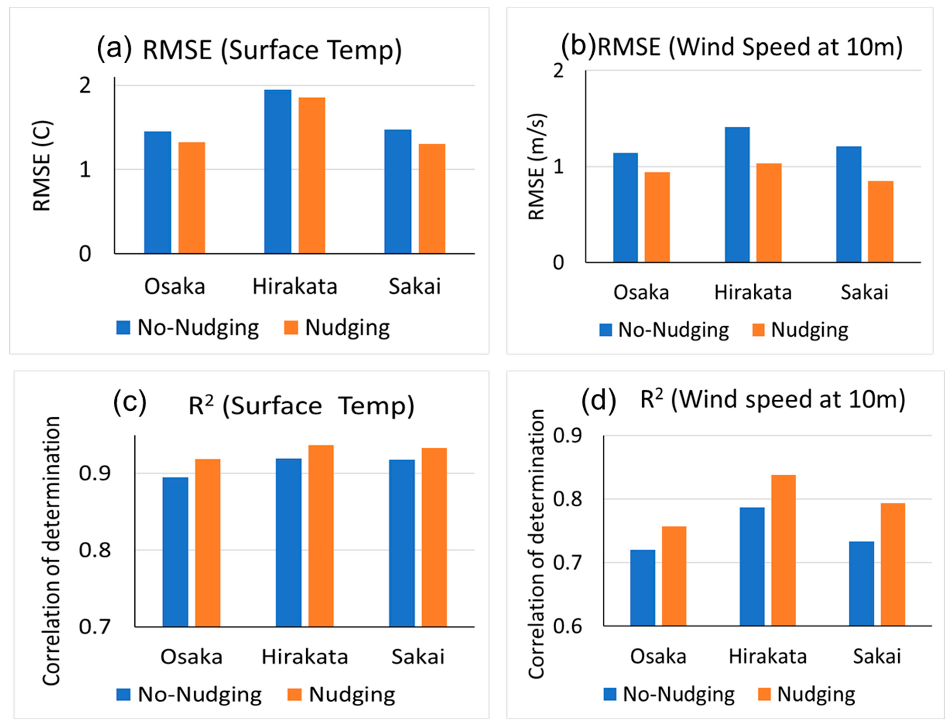
3.1. Performance Evaluation

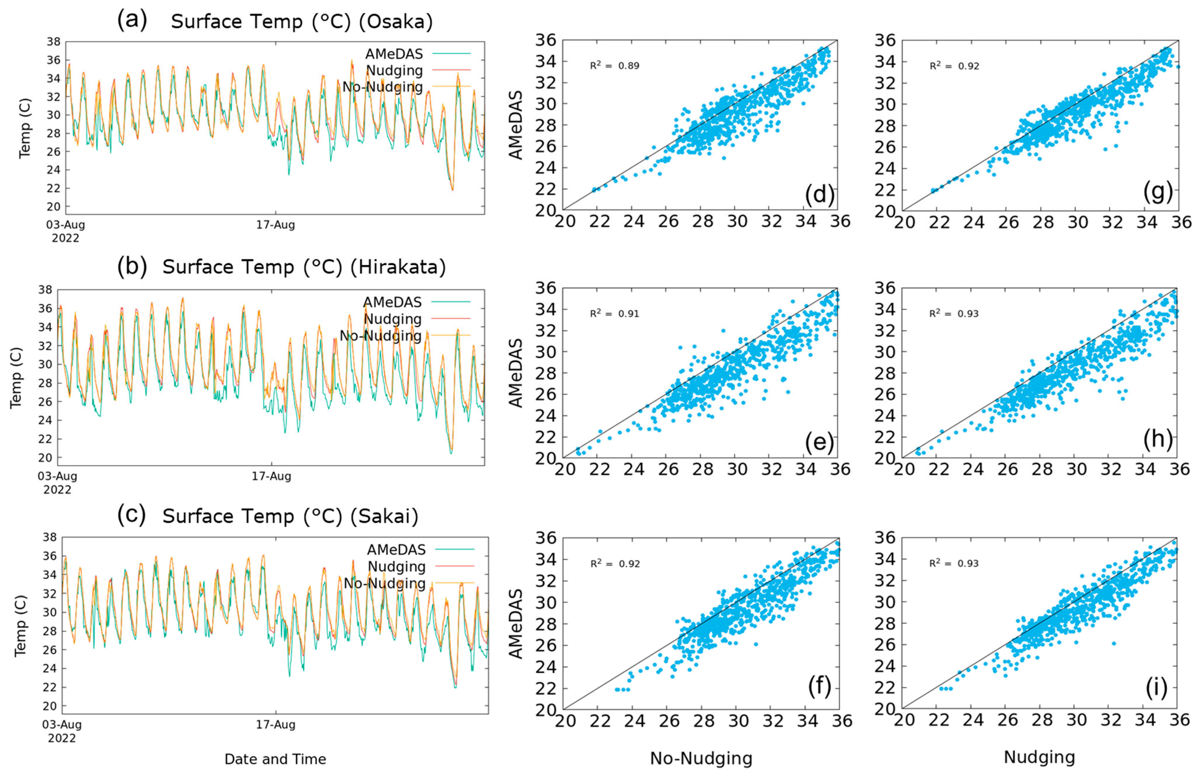
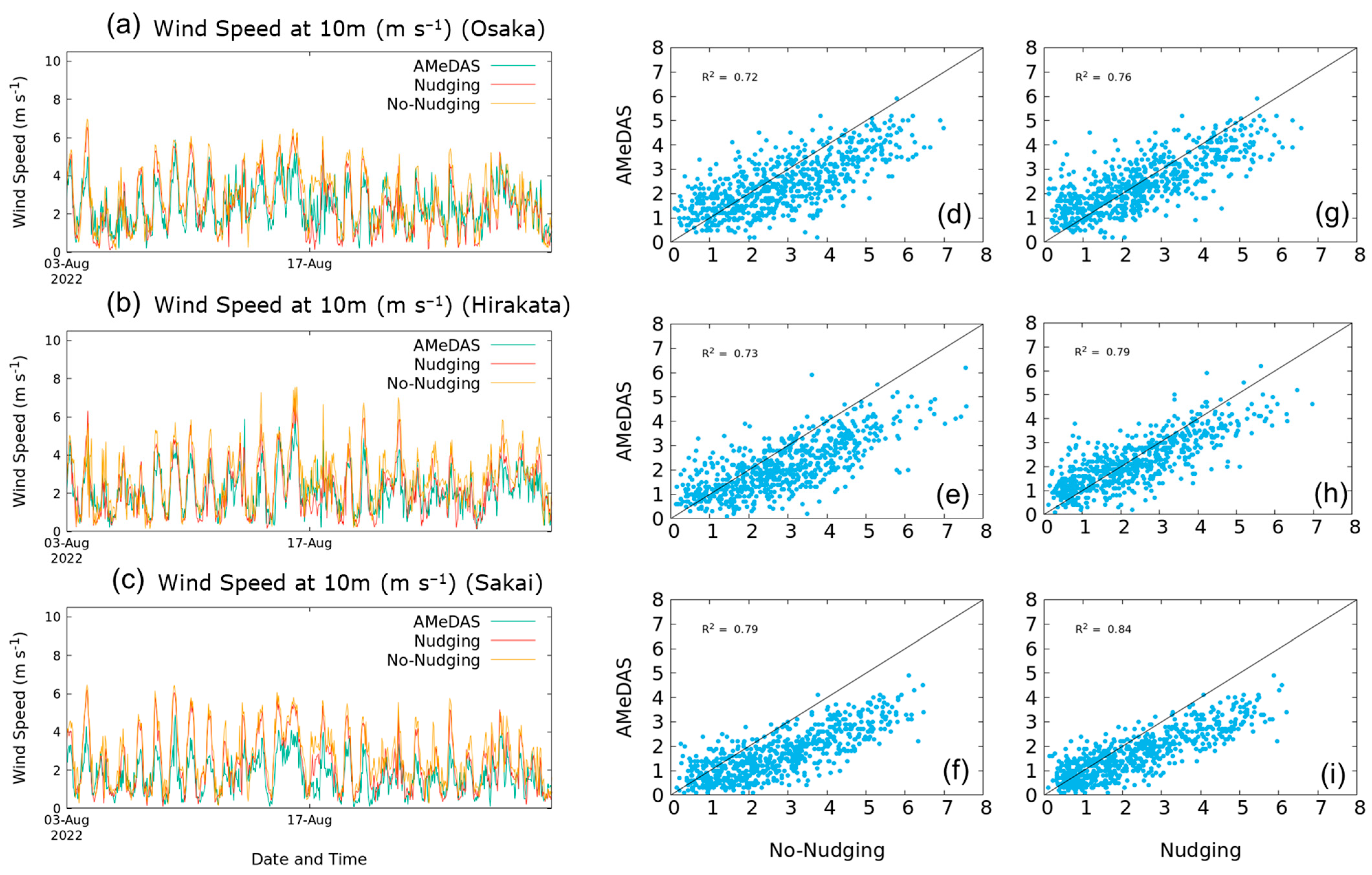
3.1.1. Comparison with AMeDAS Observation

The two simulations of the surface temperature were compared at different AMeDAS stations with and without the nudging method. The time series of the surface temperature in both simulations exhibited close agreement with slightly higher magnitudes (Figure 2), and no significant differences were found between the two simulations. However, upon closer examination, it was observed that the nudging simulation performed better than the no-nudging simulation (Figure 2a–c). These results suggest that the nudging simulation more accurately represented the temperature compared to the no-nudging simulation. Furthermore, the nudging method was found to improve the correlation between the simulated and observed temperature, with correlations improving up to 3% after using lidar-based observation nudging (Figure 2d–i).
The time series of wind speed at three AMeDAS stations were compared between the simulated and observed data (Figure 3). The results indicated that both simulations closely matched the observed wind speed, suggesting that the WRF model accurately simulated the wind speed (Figure 3a–c). However, the nudging simulation outperformed the no-nudging simulation in terms of the correlation between the simulated wind speed and the observed wind speed. Lidar-based observation nudging led to an improvement in the wind speed correlation of up to 8% (Figure 3d–i). This improvement was greater than that observed in the temperature field, which only showed an improvement of up to 3% after using nudging. These findings suggest that incorporating lidar-based observations in the WRF model through nudging may be effective in improving the accuracy of wind speed predictions for wind-related applications.
To assess the performance of the simulations, we calculated RMSE and the correlation between the hourly datasets from the simulations and the AMeDAS observations. The nudging simulation exhibited an improvement in the RMSE for hourly temperature, with reductions of up to 0.2 °C observed at all locations (Figure 4a). Furthermore, we observed an enhancement in the correlation between the observed and nudging-simulated temperature, with increases of up to 3% for hourly data (Figure 2d–i and Figure 4c). Similarly, the nudging simulation demonstrated a decrease in the RMSE for hourly wind speeds by up to 0.4 m s–1 (Figure 4b). Additionally, the correlation of the hourly wind speed increased by up to 8% after incorporating lidar-based observation nudging into the simulations (Figure 3d–i and Figure 4d). These results suggest that the nudging method is effective in enhancing the accuracy of both temperature and wind speed simulations, thus demonstrating its potential for improving the performance of WRF model simulations.

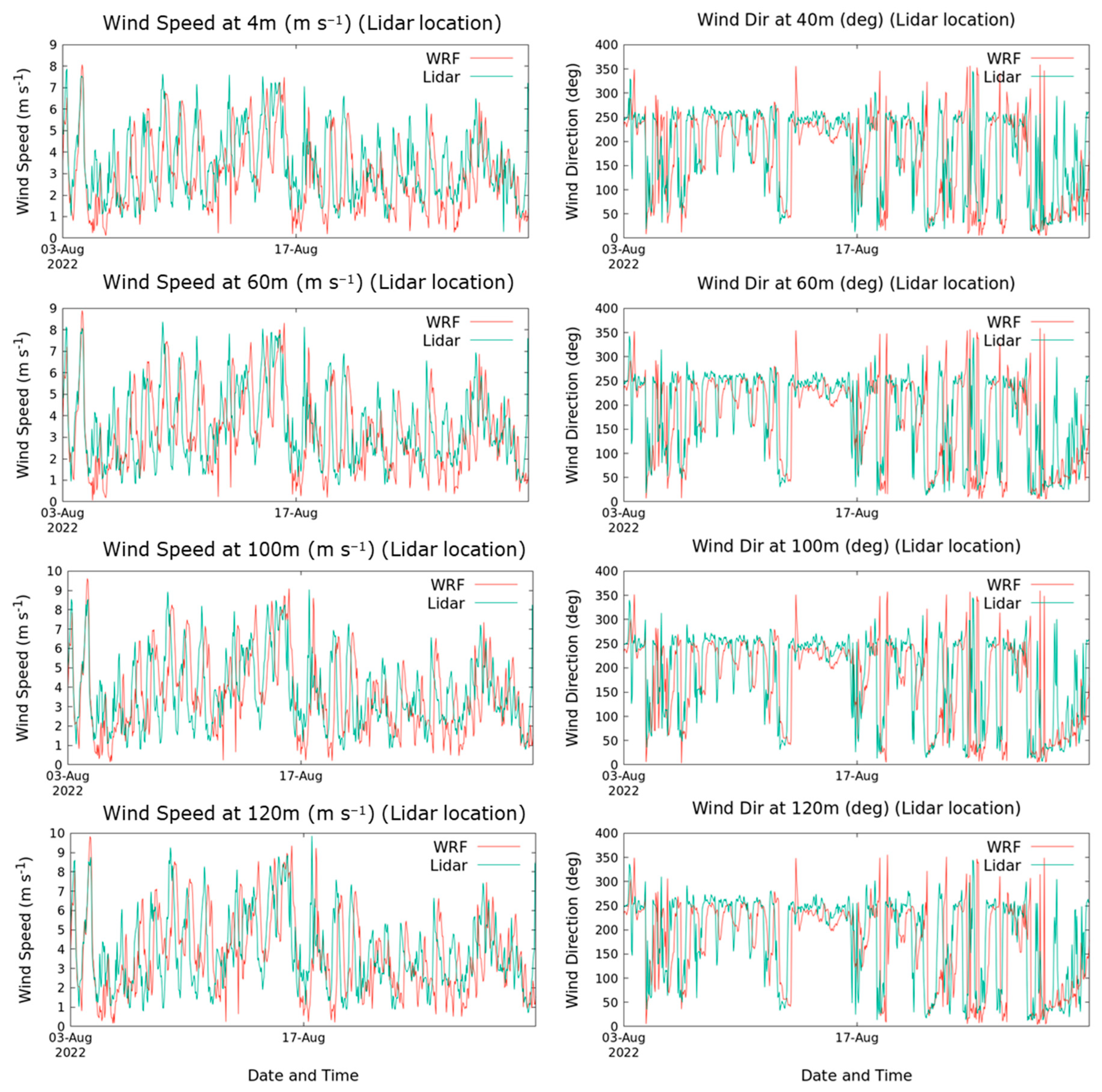
3.1.2. Comparison with Lidar Observation

The results shown in Figure 5 depict the time series of the wind speed and direction at different heights between 40 and 120 m, as observed through both the lidar and the model simulation with nudging. The results reveal that the model was able to capture the wind speed and direction closely at all heights compared to the lidar observations. However, during the end week of August, some differences were noticed in the magnitudes of the wind direction. Specifically, the model underestimated the observed magnitude of the wind direction during that period. Nevertheless, the pattern of the wind direction in the WRF model was consistent with the observations, suggesting that while the magnitudes may not have been precisely accurate, the overall pattern of the wind direction was consistent with the observations.

3.2. Analysis on the Simulated Results

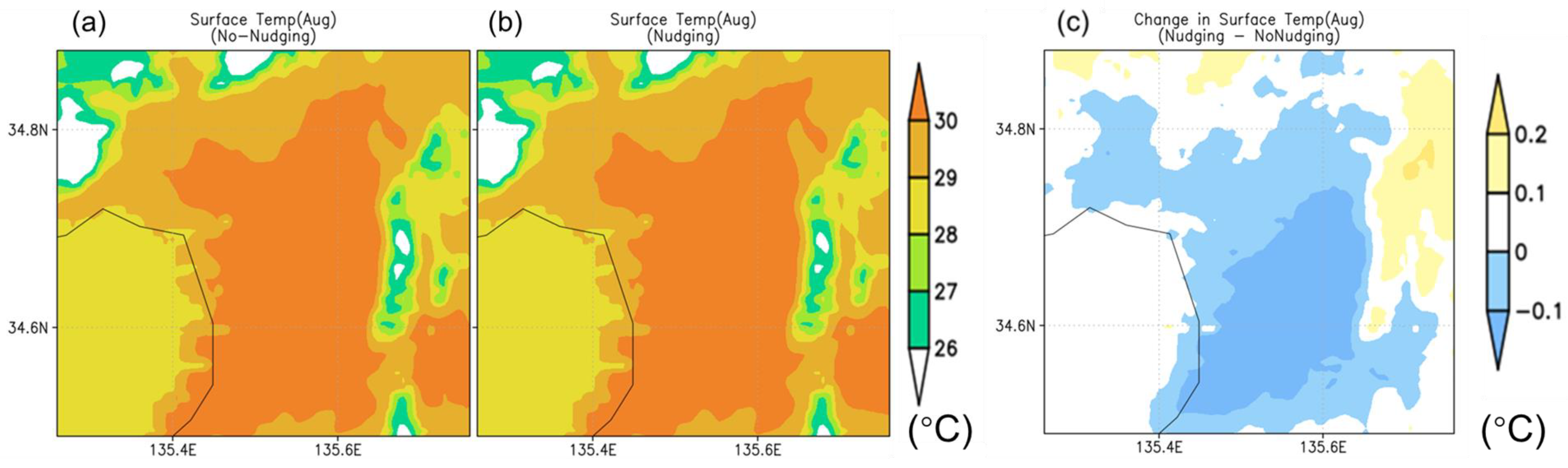
3.2.1. Surface Temperature
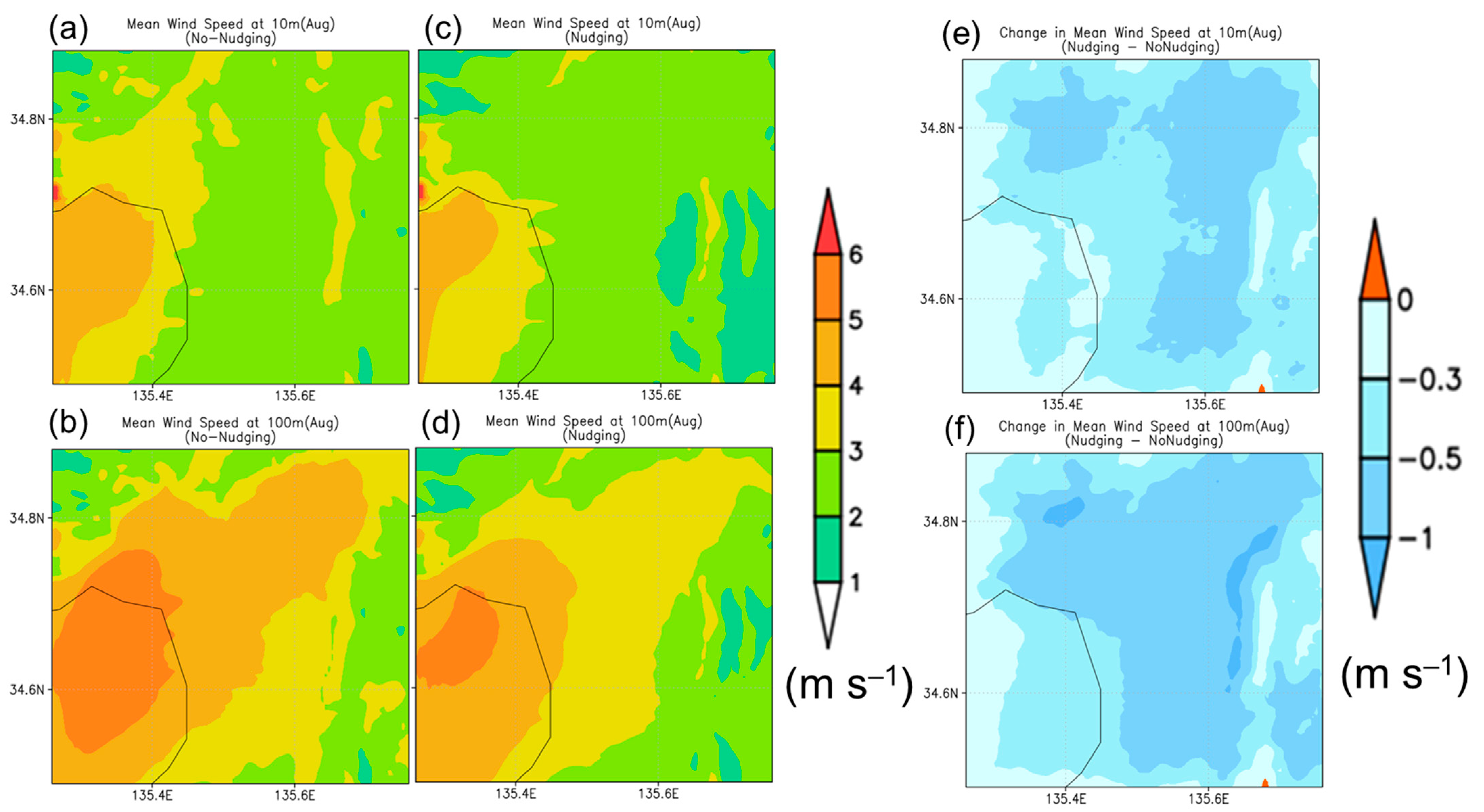
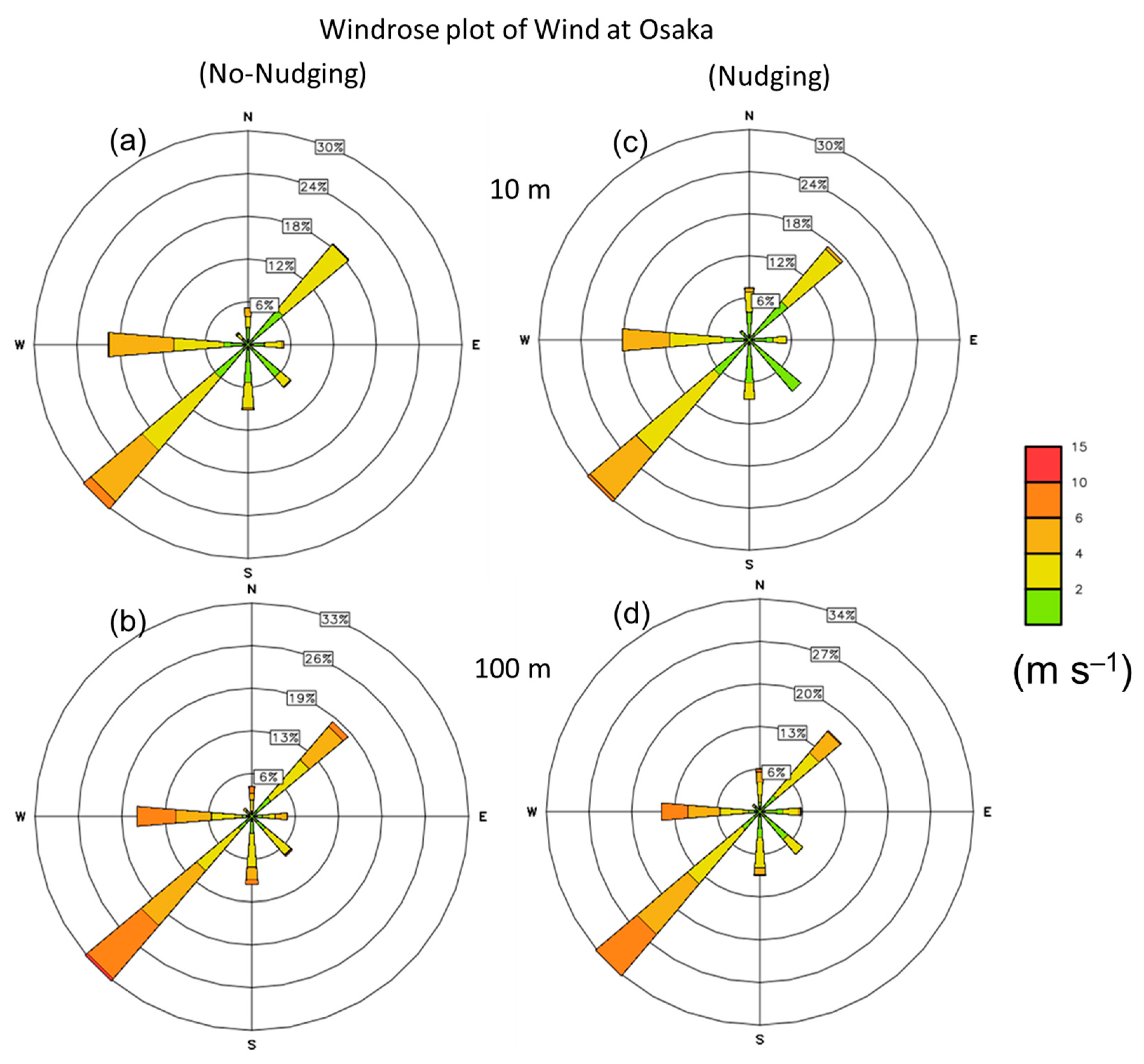
In August, the mean temperature in the Osaka region is consistently high, with temperatures in the Osaka plain region even warmer and up to 1–2 °C higher than other parts of the study area (Figure 6). The comparison of the nudging simulation with the no-nudging simulation showed that temperatures were higher in the nudging simulation over land areas over 300 m above sea level. Conversely, in lower altitude regions, the nudging simulation generally showed lower temperatures compared to the no-nudging simulation, with a few exceptions. By incorporating observation nudging, the temperature increased by 0.2 °C or more in many high-altitude regions, while it decreased by 0.1 °C or more in some coastal areas (Figure 6c). These results suggest that the use of observation nudging improved the temperature predictions in certain regions, particularly at higher altitudes.
Table 2 shows the mean biases and standard deviations in temperature at each observation location. Both simulations showed warm bias, indicating that they consistently overestimated the temperature in comparison to the observed values. However, the nudging simulation had a colder temperature than the no-nudging simulation, indicating an improvement. This suggests that the use of lidar-based observation nudging resulted in a reduction in the warm bias in the simulations. At all observation stations, the nudging simulation showed an improvement of up to 0.2 °C in the mean temperature, bringing it closer to the observed temperature than the no-nudging simulation. Furthermore, the standard deviations of temperature in the nudging simulation were generally lower than in the no-nudging simulation, with a reduction of up to 0.1 °C, approaching that in the AMeDAS observation.

3.2.2. Wind

Figure 7 shows the wind speed distribution for August 2022 at the 10 m and 100 m height levels for the simulations with and without nudging, along with the difference between them. The average wind speed over the Seto Inland Sea was approximately 4 m s–1 or higher at the 10 m height level and around 6 m s–1 or higher at the 100 m height level (Figure 7a–d). Comparing the two simulations showed that the average wind speed in the nudging simulation was lower throughout the Osaka region compared to the no-nudging simulation, indicating that observation nudging reduced the wind speed (Figure 7e–f). The mean biases and standard deviations for the wind speed were calculated for each observation location (Table 3), indicating that the WRF simulation generated stronger winds than the actual observations, with negative wind speed biases of 0.4 m s–1 at Osaka, 1.1 m s–1 at Hirakata, and 0.7 m s–1 at Sakai for all observation locations in the no-nudging simulation. However, the nudging simulation showed a nearly 0.1 m s–1 bias at the Osaka and Sakai stations and a 0.6 m s–1 bias at Hirakata. This indicates that observation nudging improved the wind speed in the simulation, resulting in weaker wind speeds than the no-nudging simulation at all observation stations. The mean improvement in wind speed was up to 0.6 m s–1.
In addition, the nudging simulation demonstrated reduced variations in the wind speed at the 10 m height level and better agreement with the AMeDAS observations at all observation stations in comparison to the no-nudging simulation. The lower standard deviation in the nudging simulation indicates that the wind speed in this case is more consistent and closer to the observed values. Notably, the standard deviation of the wind speed showed an improvement of up to 0.08 m s–1 in the nudging simulation. The Nudging simulation showed a maximum wind speed of 6 m s–1 over coastal areas at a height of 100 m, which was 1 m s–1 higher than the no-nudging simulation. These differences in wind speed at higher altitudes are crucial for applications such as aviation and wind power generation. Overall, the results, based on the surface comparison, suggest that using lidar-based observation nudging in the WRF model can improve the accuracy of wind speed predictions, which is important for planning and operating the wind related applications.

3.2.3. Vertical Profile of Wind

Figure 8 shows the vertical profiles of wind at all three AMeDAS stations. It is observed that both simulations show stronger winds, with wind speeds above 10 m s–1 at heights ranging from 10 m to 160 m in August 2022. However, the nudging simulation demonstrates relatively fewer days with winds speeds of 10 m s–1 or greater. To further investigate the impact of nudging, wind rose diagrams were plotted at all observation stations. The results indicate that the frequency of westerly and southwesterly winds with wind speeds of 10 m s–1 or higher at the 100 m height level was lower in the nudging simulation compared to the no-nudging simulation. Specifically, the frequency of westerly and southwesterly winds decreased by approximately 4% at the 10 m height level and 3% at the 100 m height level in the nudging simulation compared to the no-nudging simulation (Figure 9, Figure 10 and Figure 11). These results suggest that observation nudging can influence the frequency of strong westerly and southwesterly winds in certain regions at specific heights.
These findings suggest that the nudging simulation may result in an underestimation of the frequency of westerly and southwesterly winds, with wind speeds of 4 m s–1 for 10 m and 6 m s–1 for 100 m, when compared to the no-nudging simulation. However, the nudging simulation showed better agreement with observations at the 10 m height level (Figure 3 and Figure 7). The vertical profile and wind rose diagrams at the 10 m height level also indicated a decrease in the frequency of westerly and southwesterly winds at all stations. Based on the better performance of the nudging simulation in representing surface wind compared to the no-nudging simulation, it is reasonable to assume that the decrease in the frequency of westerly and southwesterly winds in the nudging simulation at the 100 m height level is more accurate than in the no-nudging simulation. However, to confirm this, further observation data, such as Sonde data at the 100 m height level, are required.

4. Discussion

It was observed that the simulations conducted using the WRF model displayed a warm bias in temperature and a negative bias in wind speed over the Osaka region. This means that the temperature in the WRF simulation was warmer than the actual observed temperature, and the wind speed in the WRF simulation was weaker than what was actually observed. However, after using the lidar-based observation nudging method, these biases in the temperature and wind speed were reduced. Our study found that the use of observation nudging led to a reduction in the mean bias in wind speed of up to 0.6 m s–1 and an increase in the correlation of up to 8%. This improvement is consistent with findings from previous studies conducted in other regions [28,32,39], which have also reported improvements in simulations after using observation nudging. One possible reason for the improved simulation results is that the nudging method helps to maintain the large-scale circulation features that drive weather patterns, resulting in more accurate simulations. Another reason may be the influence of observation innovations at different vertical layers within the atmosphere [35,51]. Our nudging simulation specifically utilized lidar-based upper air observations, which allowed for weighted averaged differences between the model and observation not only at the lowest model level, but also extended vertically. Overall, the use of observation nudging appears to be a valuable tool in improving the accuracy of WRF simulations.
We also conducted an analysis of atmospheric stability using the Bulk Richardson number (RiB) in both simulations in order to determine whether there were any changes in the stability. The RiB at a height (z) was calculated using the equation given by Xue et al. in [52]:
R i B = g z ( θ v θ s ) θ s ( u 2 + v 2 )
where g is the gravity, θs is the virtual potential temperature on the surface, θv is the virtual potential temperature at height z, u is the u-wind at height z, and v is the v-wind at height z. The critical value used was 0.25.
Figure 12 illustrates the RiB at a height of 10 m for both simulations with and without nudging. The nudging simulation shows positive RiB values over many of the areas, indicating statically stable flows over those regions. On the other hand, the difference between the two simulations resulted in a combination of positive and negative values over the entire domain. Further investigation and comparison with wind speed (Figure 7b) revealed that the positive RiB values were mainly observed over many areas of land where the nudging simulation showed a weaker wind speed. These positive RiB values indicate an overall decrease in statically unstable flows or an increase in statically stable flows, which is consistent with the reduced mean wind speed in the nudging simulation and a decreased negative bias in the wind speed.
Overall, our analysis indicates that the use of Doppler lidar-based observation nudging results in an improved representation of wind profile information over the Osaka region in western Japan. This improvement is reflected in a reduction in negative wind speed bias in the simulation. Although the mean bias in the wind profile over Osaka and Sakai is reduced to almost 0.1 m s–1 after observation nudging, a bias still remains over the Hirakata region, although it has been reduced to a greater extent (Table 3). One possible reason for the bias could be due to the relatively coarse grid resolution of 500 m used in our simulations. We hypothesize that simulations with higher resolutions (e.g., 100 m) could potentially further improve the wind information by capturing more detailed and localized features of the atmospheric flow. This could help to better resolve the spatial variability in the wind speed and direction.
It is worth mentioning that the results presented in this study are based on data collected for only one month during summer in a particular region. While the findings indicate that Doppler lidar-based observation nudging has some level of effectiveness in this particular month, it may not be enough to conclude whether the observed effectiveness is consistent over an extended period. Its effects may vary in different locations also. To establish the effectiveness of Doppler lidar-based observation nudging more comprehensively, it is essential to conduct further research using data from other months, seasons and locations.

5. Conclusions

This study aimed to improve the accuracy of wind profiles in the WRF model over the Osaka region of western Japan. To achieve this, a Doppler lidar was deployed and lidar-based observation nudging was used. Two simulations were conducted, one with nudging and one without nudging, and the results were compared. Both simulations produced a cold bias in temperature and a negative bias in wind speed. However, after using lidar-based observation nudging, the mean bias in temperature was reduced by up to 0.2 °C, with an improvement in correlation of up to 3%. In addition the mean bias in wind speed was reduced by up to 0.6 m s–1, with an improvement in correlation of up to 8%. The nudging simulation also showed a relatively lower RMSE and standard deviation compared to the no-nudging simulation. The overall analysis indicated that employing Doppler lidar-based observation nudging in the WRF simulation improved the wind information over the regions of Osaka and would be useful in wind-related applications and operations.

Author Contributions

S.N. proposed the topic, designed the study, analyzed the data, and drafted the manuscript. I.K. helped in the interpretation and the construction of the manuscript. All authors have read and agreed to the published version of the manuscript.

Funding

This study is supported and funded by Japan Meteorological Corporation, Japan.

Institutional Review Board Statement

Not applicable.

Informed Consent Statement

Not applicable.

Data Availability Statement

The dataset supporting the conclusions of this article are obtained from the Japan Meteorological Agency (JMA, www.jmbsc.or.jp (accessed on 15 December 2022)), Japan Meteorological Corporation (JMC, https://ods.n-kishou.co.jp/ (accessed on 15 December 2022)), National Center for Atmospheric Research (NCAR, https://rda.ucar.edu/ (accessed on 15 December 2022)), and Earthdata NASA, https://www.earthdata.nasa.gov/ (accessed on 15 December 2022)).

Acknowledgments

We acknowledge the four anonymous reviewers for their insightful suggestions to improve the quality of the manuscript. The Japan Meteorological Agency, National Center for Atmospheric Research, UK’s Met Office and NASA are acknowledged for providing the necessary datasets for this study. Yasuyuki Itano of Osaka City Research Center of Environmental Science is acknowledged for providing necessary facilities in installing the Doppler Lidar.

Conflicts of Interest

The authors declare no conflict of interest.

References

  1. Skamarock, W.C.; Klemp, J.B.; Dudhia, J.; Gill, D.O.; Barker, D.M.; Wang, W.; Powers, J.G. A Description of the Advanced Research WRF Version 3; NCAR Technical note-475+ STR; National Center for Atmospheric Research: Boulder, CO, USA, 2008. [Google Scholar]
  2. Maity, S.; Nayak, S.; Nayak, H.P.; Bhatla, R. Comprehensive assessment of RegCM4 towards interannual variability of Indian Summer Monsoon using multi-year simulations. Theor. Appl. Climatol. 2022, 148, 491–516. [Google Scholar] [CrossRef]
  3. Morimoto, J.; Aiba, M.; Furukawa, F.; Mishima, Y.; Yoshimura, N.; Nayak, S.; Takemi, T.; Haga, C.; Matsui, T.; Nakamura, F. Risk assessment of forest disturbance by typhoons with heavy precipitation in northern Japan. For. Ecol. Manag. 2021, 479, 118521. [Google Scholar] [CrossRef]
  4. Nayak, S.; Takemi, T. Robust responses of typhoon hazards in northern Japan to global warming climate: Cases of landfalling typhoons in 2016. Meteorol. Appl. 2020, 27, e1954. [Google Scholar] [CrossRef]
  5. Zhang, Q.; Tong, P.; Liu, M.; Lin, H.; Yun, X.; Zhang, H.; Wang, X. A WRF-Chem model-based future vehicle emission control policy simulation and assessment for the Beijing-Tianjin-Hebei region, China. J. Environ. Manag. 2020, 253, 109751. [Google Scholar] [CrossRef]
  6. Nayak, S.; Takemi, T. Atmospheric driving mechanisms of extreme precipitation events in July of 2017 and 2018 in western Japan. Dyn. Atmos. Ocean. 2021, 93, 101186. [Google Scholar] [CrossRef]
  7. Singh, K.S.; Nayak, S.; Maity, S.; Nayak, H.P.; Dutta, S. Prediction of Extremely Severe Cyclonic Storm “Fani” Using Moving Nested Domain. Atmosphere 2023, 14, 637. [Google Scholar] [CrossRef]
  8. Nayak, S.; Takemi, T. Dynamical downscaling of Typhoon Lionrock (2016) for assessing the resulting hazards under global warming. J. Meteorol. Soc. Jpn. Ser. II 2019, 97, 69–88. [Google Scholar] [CrossRef] [Green Version]
  9. Li, J.; Yu, S.; Chen, X.; Zhang, Y.; Li, M.; Li, Z.; Song, Z.; Liu, W.; Li, P.; Xie, M.; et al. Evaluation of the WRF-CMAQ Model Performances on Air Quality in China with the Impacts of the Observation Nudging on Meteorology. Aerosol Air Qual. Res. 2022, 22, 220023. [Google Scholar] [CrossRef]
  10. Nayak, S.; Takemi, T. Quantitative estimations of hazards resulting from Typhoon Chanthu (2016) for assessing the impact in current and future climate. Hydrol. Res. Lett. 2019, 13, 20–27. [Google Scholar] [CrossRef] [Green Version]
  11. Nayak, S.; Dairaku, K.; Takayabu, I.; Suzuki-Parker, A.; Ishizaki, N.N. Extreme precipitation linked to temperature over Japan: Current evaluation and projected changes with multi-model ensemble downscaling. Clim. Dyn. 2018, 51, 4385–4401. [Google Scholar] [CrossRef] [Green Version]
  12. Nayak, S.; Dairaku, K. Future changes in extreme precipitation intensities associated with temperature under SRES A1B scenario. Hydrol. Res. Lett. 2016, 10, 139–144. [Google Scholar] [CrossRef] [Green Version]
  13. Maity, S.; Satyanarayana, A.N.V.; Mandal, M.; Nayak, S. Performance evaluation of land surface models and cumulus convection schemes in the simulation of Indian summer monsoon using a regional climate model. Atmos. Res. 2017, 197, 21–41. [Google Scholar] [CrossRef]
  14. Tuy, S.; Lee, H.S.; Chreng, K. Integrated assessment of offshore wind power potential using Weather Research and Forecast (WRF) downscaling with Sentinel-1 satellite imagery, optimal sites, annual energy production and equivalent CO2 reduction. Renew. Sustain. Energy Rev. 2022, 163, 112501. [Google Scholar] [CrossRef]
  15. Maity, S.; Mandal, M.; Nayak, S.; Bhatla, R. Performance of cumulus parameterization schemes in the simulation of Indian Summer Monsoon using RegCM4. Atmósfera 2017, 30, 287–309. [Google Scholar] [CrossRef] [Green Version]
  16. Nayak, S.; Mandal, M.; Maity, S. Customization of regional climate model (RegCM4) over Indian region. Theor. Appl. Climatol. 2017, 127, 153–168. [Google Scholar] [CrossRef]
  17. Chen, W.; Castruccio, S.; Genton, M.G.; Crippa, P. Current and future estimates of wind energy potential over Saudi Arabia. J. Geophys. Res. Atmos. 2018, 123, 6443–6459. [Google Scholar] [CrossRef] [Green Version]
  18. Nayak, S.; Mandal, M.; Maity, S. RegCM4 simulation with AVHRR land use data towards temperature and precipitation climatology over Indian region. Atmos. Res. 2018, 214, 163–173. [Google Scholar] [CrossRef]
  19. Li, H.; Claremar, B.; Wu, L.; Hallgren, C.; Körnich, H.; Ivanell, S.; Sahlée, E. A sensitivity study of the WRF model in offshore wind modeling over the Baltic Sea. Geosci. Front. 2021, 12, 101229. [Google Scholar] [CrossRef]
  20. Mohanty, U.C.; Osuri, K.K.; Routray, A.; Mohapatra, M.; Pattanayak, S. Simulation of Bay of Bengal tropical cyclones with WRF model: Impact of initial and boundary conditions. Mar. Geod. 2010, 33, 294–314. [Google Scholar] [CrossRef]
  21. Liu, L.; Ma, Y.; Menenti, M.; Zhang, X.; Ma, W. Evaluation of WRF modeling in relation to different land surface schemes and initial and boundary conditions: A snow event simulation over the Tibetan Plateau. J. Geophys. Res. Atmos. 2019, 124, 209–226. [Google Scholar] [CrossRef] [Green Version]
  22. Gholami, S.; Ghader, S.; Khaleghi-Zavareh, H.; Ghafarian, P. Sensitivity of WRF-simulated 10 m wind over the Persian Gulf to different boundary conditions and PBL parameterization schemes. Atmos. Res. 2021, 247, 105147. [Google Scholar] [CrossRef]
  23. Srinivas, C.V.; Yesubabu, V.; Venkatesan, R.; Ramakrishna, S.S. Impact of assimilation of conventional and satellite meteorological observations on the numerical simulation of a Bay of Bengal tropical cyclone of November 2008 near Tamilnadu using WRF model. Meteorol. Atmos. Phys. 2010, 110, 19–44. [Google Scholar] [CrossRef]
  24. Shimada, S.; Ohsawa, T. Accuracy and characteristics of offshore wind speeds simulated by WRF. Sola 2011, 7, 21–24. [Google Scholar] [CrossRef] [Green Version]
  25. Singh, K.S.; Bhaskaran, P.K. Impact of lateral boundary and initial conditions in the prediction of Bay of Bengal cyclones using WRF model and its 3D-VAR data assimilation system. J. Atmos. Sol.-Terr. Phys. 2018, 175, 64–75. [Google Scholar] [CrossRef]
  26. Osuri, K.K.; Mohanty, U.C.; Routray, A.; Mohapatra, M. The impact of satellite-derived wind data assimilation on track, intensity and structure of tropical cyclones over the North Indian Ocean. Int. J. Remote Sens. 2012, 33, 1627–1652. [Google Scholar] [CrossRef]
  27. Nadimpalli, R.; Srivastava, A.; Prasad, V.S.; Osuri, K.K.; Das, A.K.; Mohanty, U.C.; Niyogi, D. Impact of INSAT-3D/3DR radiance data assimilation in predicting tropical cyclone Titli over the Bay of Bengal. IEEE Trans. Geosci. Remote Sens. 2020, 58, 6945–6957. [Google Scholar] [CrossRef]
  28. Bullock, O.R.; Alapaty, K.; Herwehe, J.A.; Mallard, M.S.; Otte, T.L.; Gilliam, R.C.; Nolte, C.G. An observation-based investigation of nudging in WRF for downscaling surface climate information to 12-km grid spacing. J. Appl. Meteorol. Climatol. 2014, 53, 20–33. [Google Scholar] [CrossRef]
  29. Mylonas, M.P.; Barbouchi, S.; Herrmann, H.; Nastos, P.T. Sensitivity analysis of observational nudging methodology to reduce error in wind resource assessment (WRA) in the North Sea. Renew. Energy 2018, 120, 446–456. [Google Scholar] [CrossRef]
  30. Ren, H.; Laima, S.; Chen, W.L.; Guo, A.; Li, H. Spatial correlation-based WRF observation-nudging approach in simulating regional wind field. Wind. Struct. 2019, 28, 129–140. [Google Scholar]
  31. Xiao, X.; Sun, J.; Ji, L.; Zhang, L.; Ying, Z.; Chen, Z.; Chen, M.; Xu, C. A Study on Local-Scale Thermal and Dynamical Mechanisms in the Initiation of a Squall Line Under Weak Forcing. J. Geophys. Res. Atmos. 2022, 127, e2021JD035561. [Google Scholar] [CrossRef]
  32. Yi, X.; Li, D.; Zhao, C.; Shen, L.; Zhou, X. Impact of a dense surface network on high-resolution dynamical downscaling via observation nudging. J. Appl. Meteorol. Climatol. 2020, 59, 1655–1670. [Google Scholar] [CrossRef]
  33. Tsujino, S.; Tsuboki, K. Intensity change of Typhoon Nancy (1961) during landfall in a moist environment over Japan: A numerical simulation with spectral nudging. J. Atmos. Sci. 2020, 77, 1429–1454. [Google Scholar] [CrossRef]
  34. Stauffer, D.R.; Seaman, N.L. Multiscale Four-Dimensional Data Assimilation. J. Appl. Meteor. 1994, 33, 416–434. [Google Scholar] [CrossRef]
  35. Deng, A.; Stauffer, D.; Gaudet, B.; Dudhia, J.; Wu, C.B.W.; Vandenberghe, F.; Liu, Y.; Bourgeoi, A. 2009: Update on WRF-ARW End-to-End Multi-Scale FDDA System. In Proceedings of the 10th WRF Users’ Workshop, NCAR, Boulder, CO, USA, 23–26 June 2009; Chapter 1.9. Available online: http://www2.mmm.ucar.edu/wrf/users/workshops/WS2009/WorkshopPapers.php (accessed on 12 April 2022).
  36. Ren, H.; Dudhia, J.; Ke, S.; Li, H. The basic wind characteristics of idealized hurricanes of different intensity levels. J. Wind Eng. Ind. Aerodyn. 2022, 225, 104980. [Google Scholar] [CrossRef]
  37. Wang, H.; Liu, Y.; Cheng, W.Y.; Zhao, T.; Xu, M.; Liu, Y.; Shen, S.; Calhoun, K.M.; Fierro, A.O. Improving lightning and precipitation prediction of severe convection using lightning data assimilation with NCAR WRF-RTFDDA. J. Geophys. Res. Atmos. 2017, 122, 12–296. [Google Scholar] [CrossRef]
  38. Li, X.; Choi, Y.; Czader, B.; Roy, A.; Kim, H.; Lefer, B.; Pan, S. The impact of observation nudging on simulated meteorology and ozone concentrations during DISCOVER-AQ 2013 Texas campaign. Atmos. Chem. Phys. 2016, 16, 3127–3144. [Google Scholar] [CrossRef] [Green Version]
  39. Sommerfeld, M.; Dörenkämper, M.; Steinfeld, G.; Crawford, C. Improving mesoscale wind speed forecasts using lidar-based observation nudging for airborne wind energy systems. Wind Energy Sci. 2019, 4, 563–580. [Google Scholar] [CrossRef] [Green Version]
  40. Lorenz, T.; Barstad, I. A dynamical downscaling of ERA-Interim in the North Sea using WRF with a 3 km grid-for wind resource applications. Wind Energy 2016, 19, 1945–1959. [Google Scholar] [CrossRef]
  41. Janjić, Z.I. The step-mountain eta coordinate model: Further developments of the convection, viscous sublayer, and turbulence closure schemes. Mon. Weather Rev. 1994, 122, 927–945. [Google Scholar] [CrossRef]
  42. Rogers, E.; Black, T.; Ferrier, B.; Lin, Y.; Parrish, D.; DiMego, G. Changes to the NCEP Meso Eta Analysis and Forecast System: Increase in resolution, new cloud microphysics, modified precipitation assimilation, modified 3DVAR analysis. NWS Tech. Proced. Bull. 2001, 488, 15. [Google Scholar]
  43. Ferrier, B.S. J4. 2 Modifications of Two Convective Schemes Used In The Ncep Eta Model. In Proceedings of the 20th Conference on Weather Analysis and Forecasting/16th Conference on Numerical Weather Prediction, Seattle, WA, USA, 10–15 January 2004. [Google Scholar]
  44. Iacono, M.J.; Delamere, J.S.; Mlawer, E.J.; Shephard, M.W.; Clough, S.A.; Collins, W.D. Radiative forcing by long-lived greenhouse gases: Calculations with the AER radiative transfer models. J. Geophys. Res. Atmos. 2008, 113, D13103. [Google Scholar] [CrossRef]
  45. Dudhia, J. Numerical study of convection observed during the winter monsoon experiment using a mesoscale two-dimensional model. J. Atmos. Sci. 1989, 46, 3077–3107. [Google Scholar] [CrossRef]
  46. Chen, F.; Dudhia, J. Coupling an advanced land surface hydrology model with the Penn State NCAR MM5 modeling system. Part I: Model implementation and sensitivity. Mon. Weather Rev. 2001, 129, 569–585. [Google Scholar] [CrossRef]
  47. Ma, H.; Cao, X.; Ma, X.; Su, H.; Jing, Y.; Zhu, K. Improving the Wind Power Density Forecast in the Middle- and High-Latitude Regions of China by Selecting the Relatively Optimal Planetary Boundary Layer Schemes. Atmosphere 2022, 13, 2034. [Google Scholar] [CrossRef]
  48. Shikhovtsev, A.Y.; Kovadlo, P.G.; Lezhenin, A.A.; Korobov, O.A.; Kiselev, A.V.; Russkikh, I.V.; Kolobov, D.Y.; Shikhovtsev, M.Y. Influence of Atmospheric Flow Structure on Optical Turbulence Characteristics. Appl. Sci. 2023, 13, 1282. [Google Scholar] [CrossRef]
  49. NASA/METI/AIST/Japan Space Systems and U.S./Japan ASTER Science Team, 2019. ASTER Global Digital Elevation Model V003 [ASTGTMv003]. NASA EOSDIS Land Processes DAAC. Available online: https://lpdaac.usgs.gov/products/astgtmv003/ (accessed on 1 April 2022).
  50. Geospatial Information Authority of Japan, GSI Web Site. Available online: https://www.gsi.go.jp/ENGLISH/page_e30233.html (accessed on 1 April 2022).
  51. Pattantyus, A. Optimizing Strategies for an Observation-Nudging-Based Four-Dimensional Data Assimilation Forecast Approach with WRF-ARW. U.S. Army Research Laboratory. Summer Research Technical Report. 2011. Available online: https://apps.dtic.mil/sti/pdfs/ADA558426.pdf (accessed on 25 August 2022).
  52. Xue, Y.; Sellers, P.J.; Kinter, J.L.; Shukla, J. A simplified biosphere model for global climate studies. J. Clim. 1991, 4, 345–364. [Google Scholar] [CrossRef]
Figure 1. Model domain with terrain height (unit: m) and the location of the Doppler lidar (red square) and the AMeDAS observation stations (black squares) (a) location map; (b) model domain with terrain height.
Atmosphere 14 00972 g001
Figure 2. Comparison of (ac) the time series of temperature for August 2022 from the model simulations with AMeDAS observation at three different stations; and (di) the correlation between them.
Atmosphere 14 00972 g002
Figure 3. Same as Figure 2, but with wind speed.
Atmosphere 14 00972 g003
Figure 4. (ab) RMSE and (cd) correlation between the model simulation and the observation from the hourly temperature (left panel) and wind speed (right panel) datasets for August 2022 at three AMeDAS observation stations.
Atmosphere 14 00972 g004
Figure 5. Comparison of the time series of wind speed (left panel) and wind direction (right panel) for August 2022 from the model simulations with lidar observation at different heights between 40 and 120 m.
Atmosphere 14 00972 g005
Figure 6. Spatial distribution of mean surface temperature for August 2022 from the simulations with (a) no nudging and (b) nudging; (c) the difference between the two simulations.
Atmosphere 14 00972 g006
Figure 7. Mean wind speed for August 2022 distribution from the simulations with (ab) no nudging and (cd) nudging at 10 m height level (upper panel) and 100 m height level (lower panel); (ef) the difference between the two simulations.
Atmosphere 14 00972 g007
Figure 8. Time series of the vertical profile of the wind speed for August 2022 from the simulations with (ac) no nudging and (df) nudging at three AMeDAS station points; (gi) the difference between the two simulations.
Atmosphere 14 00972 g008
Figure 9. Wind rose diagrams of the wind for August 2022 from the simulations with (ab) no nudging and (cd) nudging at the 10 m height level (upper panel) and 100 m height level (lower panel) at the Osaka AMeDAS station point.
Atmosphere 14 00972 g009
Figure 10. Same as Figure 8, but at the Hirakata AMeDAS station point with (ab) no nudging and (cd) nudging at the 10 m height level (upper panel) and 100 m height level (lower panel).
Atmosphere 14 00972 g010
Figure 11. Same as Figure 8, but at the Sakai AMeDAS station point with (a,b) no nudging and (c,d) nudging at the 10 m height level (upper panel) and 100 m height level (lower panel).
Atmosphere 14 00972 g011
Figure 12. Monthly mean Bulk Richardson number (RiB) distribution for August 2022 from the simulations with (a) no nudging and (b) nudging; (c) the difference between the two simulations.
Atmosphere 14 00972 g012
Table 1. Configuration of WRF.
Version3.9.1.1
Integration timeStart: 00:00 UTC 03 Aug 2022
End: 00:00 UTC 31 Aug 2022
Forcing DataLFM surface and pressure data
NCEP-FNL soil and ground data
OSTIA SST
Domain size100 × 100 (500 m horizontal grid spacing)
Vertical layer40
Model PhysicsMYJ PBL scheme [41]
Eta (Ferrier) microphysics scheme [42,43]
RRTMG longwave radiation scheme [44]
Dudhia shortwave sheme [45]
Unified Noah land-surface model [46]
FDDA optionObservation nudging was enabled in one simulation
Observation nudging was disabled in one simulation
Table 2. Mean and standard deviation of the surface temperature for August 2022 at three AMeDAS station points.
Mean (°C)
No NudgingNudgingObservationBias with
No Nudging
Bias with
Nudging
Osaka30.2730.1929.39−0.88−0.80
Hirakta30.0330.0128.50−1.53−1.50
Sakai30.5030.3529.47−1.03−0.88
Standard deviation (°C)
No NudgingNudgingObservationBias with
No Nudging
Bias with
Nudging
Osaka2.562.512.680.120.17
Hirakta3.043.082.97−0.07−0.12
Sakai2.532.662.650.11−0.01
Table 3. Mean and standard deviation of the wind speed for August 2022 at three AMeDAS station points.
Mean (m s−1)
No NudgingNudgingObservationBias with No NudgingBias with
Nudging
Osaka2.862.462.39−0.47−0.07
Hirakta2.732.291.67−1.06−0.62
Sakai2.822.262.12−0.70−0.14
Standard deviation (m s−1)
No NudgingNudgingObservationBias with No
Nudging
Bias with
Nudging
Osaka1.501.441.10−0.40−0.33
Hirakta1.471.430.94−0.53−0.49
Sakai1.461.381.06−0.39−0.31
Disclaimer/Publisher’s Note: The statements, opinions and data contained in all publications are solely those of the individual author(s) and contributor(s) and not of MDPI and/or the editor(s). MDPI and/or the editor(s) disclaim responsibility for any injury to people or property resulting from any ideas, methods, instructions or products referred to in the content.

