Abstract
On the basis of interferometry measurement made with the Chung-Li VHF radar, we investigated the effects of upward propagating gravity waves on the spatial structures and dynamic behavior of the 3 m field-aligned irregularities (FAIs) of the sporadic E (Es) layer. The results demonstrate that the quasi-periodic gravity waves oscillating at a dominant wave period of about 46.3 min propagating from east-southeast to west-northwest not only modulated the Es layer but also significantly disturbed the Es layer. Interferometry analysis indicates that the plasma structures associated with gravity wave propagation were in clumpy or plume-like structures, while those not disturbed by the gravity waves were in a thin layer structure that descended over time at a rate of about 2.17 km/h. Observation reveals that the height of a thin Es layer with a thickness of about 2–4 km can be severely modulated by the gravity wave with a height as large as 10 km or more. Moreover, sharply inclined plume-like plasma irregularities with a tilted angle of about 55° or more with respect to the zonal direction were observed. In addition, concave and convex shapes of the Es layer caused by the gravity wave modulations were also found. Some of the wave-generated electric fields were so intense that the corresponding E × B drift velocities of the 3 m Es FAIs approximated 90 m s−1. Most interestingly, sharp Doppler velocity shear as large as 68 m/s/km of the Es FAIs at a height of around 108 km, which bore a strong association with the result of the gravity wave propagation, was provided. The plausible mechanisms responsible for this tremendously large Doppler velocity shear are discussed.
1. Introduction
The sporadic E (Es) layer is a thin layer that is composed of long, live metallic ions (such as Fe+, Ca+, and Na+) of meteoric origin and it is usually found in the altitude ranges of about 90–130 km. Recently, Es and sporadic metal layers have been studied simultaneously to understand their relationships [,,,]. The ionospheric sporadic E (Es) layer and irregularities have been investigated extensively, both theoretically and experimentally. Different observational techniques, such as ionosondes, coherent scatter radars, incoherent scatter radars, satellite, and in situ sounding rockets, have been widely used to investigate ionospheric electron density irregularities [,,,,,,]. Because of its highly magnetized property and quasi-equal potential line approximation to the magnetic field line in the ionosphere [], free electrons can move almost freely along the magnetic field line, and the electron densities have a nearly uniform distribution along the magnetic field line. However, because of the plasma turbulence cascade process [], the electron density distributions across the local magnetic field line highly fluctuate. As a result, the radar backscatter from the spatial variations of electron densities at the Bragg scale can only be detected in the direction nearly perpendicular to the local magnetic field line [,,]. The electron density irregularities with this property are called field-aligned irregularities (FAIs). The angular span of the radar returns distributed with respect to the radar wave vector normal to the local magnetic field line is called the aspect angle of the FAI backscatter, which is usually smaller than 0.2° [].
The physical processes that are responsible for the generations of the sporadic E (Es) irregularities or Es layers vary with geomagnetic latitudes. For example, the wind shear theory accounting for the formation of the Es layer can only apply to those at low and mid-latitudes [,,]; the plasma instabilities (e.g., gradient-drift instability and two-stream instability) are the major drivers for the excitations of the Es irregularities at the geomagnetic equator and in the auroral oval zone [,,,]; the Es irregularities caused by particle bombardment can only occur at a high latitude, where the magnetic field lines are characterized by very large dip angle to facilitate particle precipitations from the magnetosphere and plasmasphere [,]. No matter what the physical process is, the meter-scale Es irregularities at different latitudes are essentially field-aligned irregularities (FAIs) and can only be observed by using a ground-based VHF coherent scatter radar in the direction of nearly normal to the local magnetic field line with aspect angles generally less than 0.5° [,]. This universal property of the Es FAIs signifies the importance of estimating the expected echoing region in the determination of the true location of the Es FAIs in the echoing region to mitigate the radar system phase bias effect on the observed radar echoes when the interferometry technique is employed [,].
Coherent and incoherent scatter radars have been widely used to study the gravity wave effect on the ionospheric Es layer. For example, Van Eyken et al. [] employed Malvern incoherent scatter radar to study the response of the Es layer to an upward propagating gravity wave group event. Bourdillon et al. [] employed a 9 MHz HF coherent scatter radar to observe quasi-period oscillations of Doppler velocity and echoing region to investigate the gravity wave modulation effect on the Es layer. Patra et al. [] observed quasi-periodic (QP) Es echoes with a period of about 2–4 min in the low E region (below 93 km) and surmised that the QP echoes were associated with Kelvin–Helmholtz (KH) instability. Chu et al. [] analyzed range-extended Es echoes measured by a 30 MHz radar and found gravity wave-induced downward phase progression of the Doppler velocities of the FAI echoes with salient wave-induced zonal displacement and indistinct modulation in height. It is noteworthy that, although the gravity wave modulation effect has been employed to account for the quasi-periodic (QP) echoes of the Es layer [,], theoretical simulations and experimental results have shown that the patchy plasma structures moving horizontally and quasi-periodically through the echoing region are very likely the major cause of the QP echoes [,,].
In order to position the FAIs in the echoing region, the use of interferometry technique to analyze and estimate the angle of arrival of the radar returns from FAIs is required. It is noteworthy that because of the radar system phase bias effect, the estimated locations of the FAIs may deviate from their true locations in the echoing region. Chu and Wang [] compared the observed FAI echoing region to the expected FAI echoing region to estimate the plausible effect of the system phase bias on the observed FAIs locations. Many researchers have applied interferometry techniques to the coherent scatter radars for the investigation of spatial structures of field-aligned Es irregularities [,,,,,,,,,]. It has been shown that the spatial structures of the Es 3 m FAI echoing region can be categorized into three types, namely, a thin horizontal layer [,,], a well-organized blob (or clump) shape [,,], and a loose cluster []. Although it has been confirmed that the layer-type Es plasma structure is the result of ion convergence caused by neutral wind shear (e.g., Chu et al. []), the physical process of generating clump-type Es structures has not been documented and well understood. In this study, employing the Chung-Li VHF radar, the observational evidence is provided to associate the Es plasma structure categorized into clump type and loose cluster type with the effects of the gravity wave breaking. In addition, an attempt is made in this article to investigate the responses of the Es layer structures to the modulation of an upward propagating inertial gravity wave in the Es region, in which the drift velocity of the Es 3 m FAIs and the three-dimensional spatial structure of the Es layer are especially concentrated.
It is generally believed that a vertically propagating gravity wave could modulate the Es layer not only in height but also in its electron density. In addition, the polarized electric field inside the Es layer, which is generated by the gravity wave-associated neutral wind through a differential collision between ion and electron, is also subject to a quasi-periodic oscillation. As a result, a quasi-periodic oscillation in the E B drift is produced, and that is responsible for the Doppler velocity of the 3 m FAIs. Nevertheless, the wave-induced horizontal modulation of the Es layer has not been well documented. An attempt is made in this article to investigate the quasi-periodic oscillations of the three-dimensional drift velocities of the 3 m FAIs of a thin Es layer observed by the Chung-Li VHF radar with interferometry measurement, which are believed to be associated with an upward and northward propagating inertial gravity wave. The observational evidence of the wave-modulating drift velocity components is presented, and their phase relations are examined in accordance with the theoretical polarization relation of the gravity wave. This paper is organized as follows. A background of interferometry measurement and experimental setup are introduced in Section 2. The observational results are presented in Section 3. Discussion and conclusion are provided in Section 4.
2. Experimental Setup
The operational frequency of the Chung-Li VHF radar is 52 MHz (corresponding to a wavelength of 5.77 m). The antenna array used exclusively for interferometry measurements of ionospheric irregularities in the Chung-Li VHF radar antenna field consists of three rectangular antenna subarrays arranged as an isosceles triangle in shape, and each subarray is composed of 32 (4 × 8) linearly polarized 4-element Yagi antennas. The side lengths of the triangle are d12 = d13 = 37.1 m and d23 = 18 m, respectively. The boresight of the antenna beam of each antenna subarray is pointed in the direction of 19.16° west of geographic north in azimuth and 50.2° in elevation. The 3 dB beam width of the two-way antenna pattern of each subarray is 7.8° in elevation and 18° in azimuth []. The configuration of the ionospheric antenna array of the Chung-Li VHF radar is shown in Figure 1.
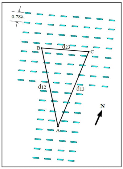
Figure 1.
Configuration of ionospheric antenna array of the Chung-Li VHF radar.
In order to perform an interferometry experiment, the phase differences of the radar returns between a pair of adjacent antenna subarrays is measured in accordance with the following expression []:
where Vp() and Vq() are the Fourier transforms of the echo signal for pth and qth receiving channels, respectively, ∗ is the complex conjugate, is the Doppler frequency, < > is the ensemble average, |Spq()| is the coherence, and ∆φpq is the phase difference between the pth and qth receiving channels (i.e., ∆φpq = φq − φp). For the Chung-Li VHF radar, from the phase differences ∆φ21 and ∆φ32 for antenna pairs (2,1) and (3,2), the elevation angle θ and azimuth angle of the target with respect to geographic north can be obtained as follows []:
where k is the radar wave number (2π/λ); λ is the radar wavelength; and represent the system phase biases for antenna pairs (2,1) and (3,2), respectively, β = 14.04°; m and l are the interferometry lobe numbers in azimuth and vertical directions, respectively, which resulted from the phase ambiguity of the radar returns received by the ionospheric array with a relatively large ratio of baseline distance and radar wavelength []. For the ionospheric antenna array of the Chung-Li VHF radar, m = 0 and l = 4. The use of the International Geomagnetic Reference Field (IGRF) model in combination with the physical antenna beam pattern can determine the expected echoing region of the field-aligned irregularities, in which the aspect angle and the height range of the FAIs are provided. By comparing the observed echoing region and the expected echoing region, we can acquire and . Details on the calibration of the system phase biases refer to Wang and Chu [].
Because of the field-aligned property of the ionospheric electron density irregularities at meter scale, the backscatter from the 3 m FAIs can only be detected and analyzed by a VHF radar within a specific echoing region that is determined by the physical antenna beam pattern and the aspect angle. This region is referred to as the expected echoing region thereafter that designates the potential echoing region of the ionospheric FAIs, which can be acquired from the International Geomagnetic Reference Field (IGRF) model combined with the geographic coordinate of the radar station [,,]. In other words, the expected echoing region is determined by the effective antenna beam pattern that is defined as the product of the transmitted (physical) radar beam pattern and aspect sensitivity of the FAI backscatter. Every coherent scatter radar has its own unique expected echoing region that stipulates a specific region where the ionospheric FAI echoes can be detected by the radar. In light of the fact that the aspect angle is usually very small (usually less than 0.2°) [], the expected echoing region is anticipated to be relatively broad in the geomagnetic zonal direction and very narrow in the geomagnetic meridional direction. Figure 2 shows the expected echoing region of the ionospheric antenna array of the Chung-Li VHF radar, in which the aspect angle of 0.2° is set and the height range of 90–130 km for the presence of FAIs is assumed. As anticipated, the configuration of the expected echoing region of the Chung-Li VHF radar is a concave down region extending in a geomagnetic zonal (azimuth) direction and restricted in the geomagnetic meridional (elevation) direction. Therefore, it is expected that the interferometry-resolved FAI echoes for the Chung-Li VHF radar should be within this highly anisotropic echoing region.
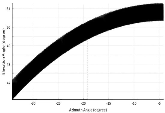
Figure 2.
Expected echoing region of the field-aligned irregularities of the Es layer in height range of 90–130 km for the ionospheric antenna array of the Chung-Li VHF radar. The aspect angle of 0.2° and azimuthal angle range from −4.8° to −40° are employed to calculate the expected echoing region from IGRF model, where negative sign of the azimuth angle signifies west to due north. The dashed vertical line at azimuth angle of −19.16° is the pointing direction of the boresight of antenna beam.
The data used for this study were taken by the Chung-Li VHF radar on 3 July 2018. To reconstruct the three dimensional spatial structures of Es irregularities with interferometry measurement, the three rectangular antenna subarrays were operated simultaneously. The radar parameters were set as follows. The transmitted peak power was 40 kW, the inter-pulse period was 5 ms, the pulse length was 8 µs, 13-bit Barker code was used for the radar pulse transmission, coherent integration was performed twice, and the probing range was set from 110.4 km to 156 km with a range resolution of 1.2 km, in which 39 range gates were sampled. A 256-point Fast Fourier Transform (FFT) algorithm was used to compute the Doppler spectra of the received signals. Five successive raw spectra were employed for performing ensemble averages of the normalized complex cross-spectrum in accordance with Equation (1) to obtain the phase difference of the Es FAI echoes between each pair of the receiving channels with a time resolution of 12.8 s. The azimuth and elevation angles of the Es irregularities were computed from the phase differences in accordance with Equations (2) and (3), in which the data were selected if the coherences |Spq()| ≥ 0.8 and |∆φ12 + ∆φ32 − ∆φ31| ≤ 3°. After the determination of the arrival angles of the Es FAI echoes, the position of the Es plasma structures in the expected echoing region can be constructed in corporation with the range.
3. Observational Results
Figure 3 shows that the range-time-intensity contour plot of the Es layer echoes observed by the Chung-Li VHF radar echoes on 3 July 2018, from 19:10 to 23:58 LT. The main body of the Es echoes descended from 148 km to 132 km at a mean range rate of 3.2 km/h. It is important to note that a 13-bit Barker code was employed to observe the Es FAI echoes in the radar experiment. As a result, unnatural echoes induced by the side lobe of the autocorrelation function of the Barker code were present symmetrically on the upper and lower sides of the main echo regions, which are 22.3 dB weaker than the main echoes. These artificial echoes should be carefully identified and removed from the raw data such that the true Es layer echoes can be correctly analyzed and the Es FAIs can be positioned in the expected echoing region using the interferometry technique. As shown in Figure 3, the whole sequence of the Es FAI echoes consists of four individual segments, in which evident quasi-periodic oscillations not only in FAI echo intensity but also in range extent can be clearly seen. The oscillation periods of the first and second segments are, respectively, about 20 min and 9.5–17.5 min with large oscillation amplitudes, while those of the third and fourth segments with minor oscillation amplitudes are short (less than 9 min) and varied. These features seem to suggest that the causes of the quasi-periodic oscillations of the Es FAI echoes are very likely the results of propagating gravity waves with different periods. In the following, using the interferometry technique mentioned in Section 2, three-dimensional spatial structures of the FAIs echo regions are reconstructed to investigate the responses of the Es layer to the propagations of the gravity waves effect, including modulation of the Es layer, change in the shape of the Es FAI echoing patterns, and the dynamic behavior of the FAIs caused by the gravity-wave-induced polarized electric field and propagation.
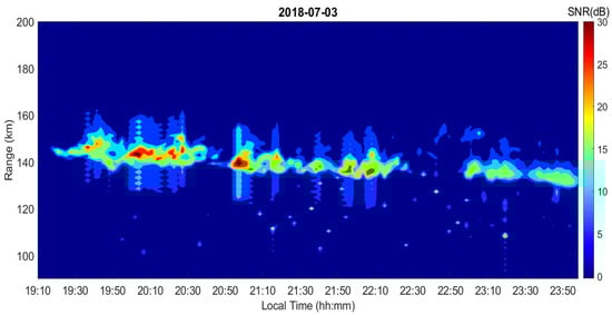
Figure 3.
Range-time-intensity contour plot of the Es FAI echoes observed by Chung-Li VHF radar on 3 July 2018. The artificial echoes caused by the sidelobe of the autocorrelation function of the Barker code, which symmetrically distribute in range above and below the main echo regions, are clearly seen.
Figure 4 displays the time sequences of interferometry-resolved echoing regions projected on vertical (top), azimuth (or zonal) (middle), and meridional (bottom) planes, respectively, in which the Doppler velocities are superimposed on the echoing regions to indicate the dynamic property of the 3 m Es FAIs. In the top panel of Figure 4, there is a trend for the main body of the Es layer to descend at a lapse rate of about 2.17 km/h, which is basically in line with the downward phase velocity of semi-diurnal tide [,,]. In addition to the steadily descending Es echoes, the observed Doppler velocities of Es FAI echoes show prominent quasi-periodical variations. Moreover, height-extended echo bulges occurred quasi-periodically during the period from 19:30 to 22:20 LT, which are consistent with those present in Figure 3. All of these features, combined with the quasi-periodic oscillations in the echo intensities present in Figure 3, strongly suggest that the Es FAIs were subjected to a forcing of external wave-like events to move alternately away and towards the radar quasi-periodically. The major causes of these quasi-periodical oscillations in the Es FAI echoes are very likely the atmospheric gravity waves propagating through the Es layer, which will be shown in a later section.
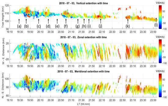
Figure 4.
Time sequences of spatial distributions of the interferometry-resolved Es FAI echoes projected on vertical (top panel), azimuth (middle panel), and horizontal (bottom panel) planes, in which Doppler velocity of the echoes are displayed in color. Positive (negative) sign on ordinate of azimuth plane indicates east (west) of the boresight of radar beam, and the numbers labeled on the ordinate of horizontal plane represent the distances of the FAI echoes north of the radar site.
In Figure 4, the Es FAI echo structures for the first segment during 19:15–20:50 LT were very complicated and disorganized. During this period, vigorous fluctuations can be found not only in Doppler velocity but also in echo intensity and spectral width, as shown in Figure 5. From the displacements of the FAI echoes on azimuth and horizontal planes over time presented in the middle and bottom panels of Figure 4, it is clear to see that the FAIs for the first half (19:15–20:10 LT) of the first segment were moving predominantly from northwest to southeast, and the FAIs for the second half (20:10–20:50 LT) of the segment were mostly moving from southeast to northwest. These two waves propagating in opposite directions interacted together during the period 19:50–20:10 LT to result in severe perturbations of the Es FAIs. At the beginning of the second segment at around 20:50 LT, another gravity wave propagation event emerged, which propagated predominantly northwest as well. Examination shows that this wave event consisted of 20 or more salient wave fronts in the trails behind the first one, which was passing through and intercepted by the expected echoing region to form striation-like echoing regions. From the displacement of the FAI echoes over time, we obtain the zonal and meridional velocity components of the FAI echoes are 55.8 m/s and 16.7 m/s, respectively, which correspond to a wave vector with a velocity of about 16 m/s and propagation direction of about 16.5° with respect to the westward direction. After 22:50 LT, the third and fourth gravity wave events can be seen. However, the FAI echo patterns of these two wave fronts were different from those in the first and second wave events, i.e., no echo bulge was found, and the separations between echo striations were indistinctive.
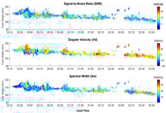
Figure 5.
Height-time distributions of the intensity (top), Doppler velocity (middle), and spectral width (bottom) for the echoes presented in Figure 4.
These echo bulges shown in Figure 3 and Figure 4 are characterized by intense echo intensities, large height extents, strong Doppler velocity, and broad spectral width, which can be seen in Figure 5. Some of them are marked with arrows and labels (b), (d), (f), (h), (j), and (k) in Figure 4 for further comparisons. Besides the echo bulges, quasi-periodic modulations of the Es echoes in height can also be discerned, although they are minor and weak. The middle and bottom panels of Figure 4 exhibit zonal and meridional movements of the Es FAI echoes over time, in which 0 km labeled on the ordinate of the azimuth plane indicates the boresight of the radar beam and positive (negative) values represent the distances of the FAI echoes away from the boresight toward east (west). The numbers labeled on the ordinate of the meridional plane represent the distances of the FAI echoes north of the radar site. It has been shown that the plasma structures responsible for the striation-like Es FAI echo patterns on the zonal or meridional planes should be a moving thin Es layer intercepted by the expected echoing region, and those in a blob shape are the result of a moving plasma structure in a clump type intercepted by the expected echoing region []. Therefore, the plasma structures responsible for the Es FAI echoes for the present study are varied and diverse.
Figure 6 demonstrates 12 selected examples of the spatial distributions of the Es FAI echoes projected on two mutually perpendicular planes, namely, vertical (top) and zonal (bottom) planes. The times that the Es FAI echoes are selected are indicated by the arrows shown in Figure 4, which cover four segments of FAI echoes shown in Figure 3 and include the echo bulges and the FAI echoes without echo bulges for comparison. Two slant lines on vertical planes are the radar wave vectors pointing toward magnetic north with elevation angles of 49° and 52°, respectively. As shown, the Es layer structures responsible for the FAI echoes that occurred between the echo bulges are horizontally stratified thin layers with thicknesses of 1.5–4 km, which are marked with the symbol ①. This feature suggests these Es layers are very quiet and steady without noticeable disturbances, which are believed to originate from the plasma convergence caused by neutral wind shear of the background semi-diurnal tide. However, the plasma structures responsible for the echo bulges are diverse, including appreciably inclined layers against horizontal plane (cases (b) and (f)), clump-type (cases (h)), and plume-type FAIs (cases (b), (d), and (f)). It is important to note that the clump-type irregularities are characterized by a quasi-isotropic blob in shape with similar dimensions in vertical and horizontal directions, while the plume-type irregularities are characterized by an anisotropic shape with a distinctive major axis. These two types of FAI echo structures are, respectively, marked with ② and ③ in Figure 6. It is noteworthy that the FAI echo structures ① and ② for case (b) at time 19:42:04 LT are appreciably tilted, making angles of 55° relative to the west for the anisotropic structures ② and 16° relative to the east for the thin Es layer ①. The detailed evolution of the echo structures for case (b) that bears a strong association with the propagation of gravity wave will be presented later. All of these features suggest that highly irregular Es FAI plasma structures in shape and severely disturbed plasma irregularities are responsible for the formation of the echo bulges, which are closely associated with external wave-like forcing to deform and perturb the Es layers.
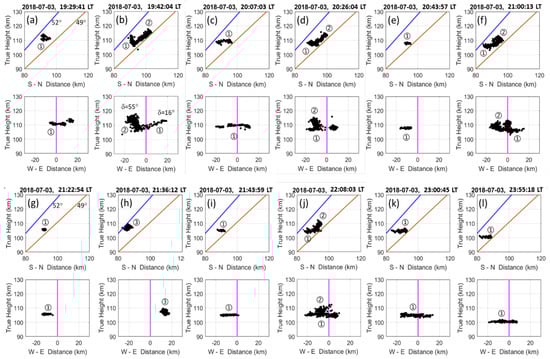
Figure 6.
Examples of interferometer-resolved Es FAI echo regions projected on vertical (with vertical and S-N coordinates) and zonal (with vertical and W-E coordinates) planes at selected times. Two straight lines inclined from upper right to lower left on the vertical planes represent radar wave vectors with elevation angles of 49° and 52°, respectively. The vertical line on the zonal plane represents the projection of the boresight of the radar beam. The symbols ①, ②, and ③ represent background Es layers formed by semi-diurnal tide, plume-like and clump-type FAIs associated with the propagations of active gravity waves, respectively.
In order to realize the wave property of the quasi-periodical oscillations in height and Doppler velocity of the Es FAI echoes, the relations between the drifting velocity components of the Es FAI echoes in different directions should be examined. On the basis of the displacements of the FAI echoes over time, as shown in Figure 4, the vertical, zonal, and meridional components of the drift velocities can be estimated. It is noteworthy that although the Doppler velocity of the FAI echoes is determined by the polarized electric field through the E × B drift effect, the bulk movements of the FAI echoes in the expected echoing region across the magnetic field lines are dominated by neutral wind through the collisions between ion and neutral particles []. Figure 7 presents the time series of the drift velocity components in zonal (blue curve), meridional (black curve), and vertical (red curve) directions. As shown, irrespective of the presence of a trend in the zonal drift velocity, there is a 90° phase difference between zonal and meridional drift velocities, while out of phase between vertical and meridional drift velocities. The primary periods of the oscillations in the drift velocity components are very consistent and around 46.3 min. This property suggests that the major cause of the quasi-periodic oscillations of the wave-like Es FAI echoes can be attributed to the vertically upward propagating gravity waves [,].
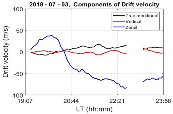
Figure 7.
Time series of the drift velocity components of FAI echoes in zonal (blue curve), meridional (black curve), and vertical (red curve) directions, which are estimated from the movements of the echoes in respective directions over time, as shown in Figure 4.
Figure 8 shows the sequential evolution of three-dimensional spatial structures of the Es layer perturbed by gravity waves in increments of about 3.5 min, in which δ is the tilt angle of the wave-deformed Es layer or plume-like plasma irregularities with respect to westward or eastward directions. Dashed lines in the zonal and horizontal planes represent projections of a horizontally stratified thin Es layer intercepted by the expected echoing region on respective planes. Therefore, the Es FAI echoes distributed along the dashed lines can be regarded as the echoes from the 3 m FAIs embedded in the horizontal thin Es layer, and those with other patterns should be caused by either deformed layers or large-scale plasma irregularities in various shapes, such as isotropic or anisotropic structures. The FAI echo regions marked with ①, ②, and ③ denote the echoes associated with the horizontal thin Es layer and the anisotropic plasma irregularities, respectively. Symbol ① signifies the background Es layer formed by the semi-diurnal tide, and ② and ③ represent plume-like or clump-type FAIs with negative and positive Doppler velocities, respectively. From their Doppler velocity distributions at time 19:38:10 LT shown in Figure 4, the FAIs marked with ② showed a downward and southeastward drift with negative Doppler velocity of about −20 m/s, while those marked with ① and ③ were moving southeastward, associated with negative and positive Doppler velocities of −55 and 10 m/s, respectively. However, just 3 min later, at 19:41:24 LT, the Doppler velocity of ③ increased dramatically from 10 m/s to 50 m/s or more and extended upward from 113 km to 117 km. At this time, irrespective of their opposite Doppler velocities, the irregularities ② and ③ merged together to form a long and slanted anisotropic irregularity with dimensions of about 12 km in zonal, 8 km in meridional, and 10 km in vertical directions, which was inclined toward the east at an angle of about 36° relative to the westward direction. In Figure 8, it is clear to see that the merged irregularity marked with ② and ③ moved southeastward, and its tilted angle varied over time from about 20° at 19:38:10 LT to 50° at 19:48:01 LT to 22° at 19:54:27 LT. In addition, Figure 8 shows that at time 19:54:27 LT, the irregularities marked with ① started to reorganize to form a concave layer structure with different Doppler velocities in it, namely, positive at west end and negative at boresight, which are opposite to those just 3 min earlier. This type of quasi-periodic change in Doppler velocities signifies the result of gravity wave propagation.
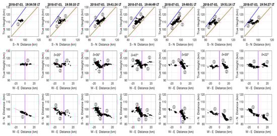
Figure 8.
Sequential evolution of three-dimensional spatial structures of Es FAIs perturbed by gravity waves in increment of about 3.5 min, in which δ is tilt angle of the wave-deformed Es FAIs with respect to westward direction. The dashed lines are the projections of a horizontally thin Es layer intercepted by the expected echoing region on respective planes. Symbol ① signifies background Es layer formed by semi-diurnal tide, and ② and ③ represent plume-like or clump-type FAI irregularities with negative and positive Doppler velocities, respectively. For detailed descriptions of the evolutions of the plasma irregularities responsible for the FAI echoes, see the text.
In addition to the gravity wave-associated plume-like or clumpy plasma irregularities, the thin Es layers that are modulated and deformed in concave or convex shape patterns were observed. Figure 9 presents four examples of the spatial structures of the Es layers severely modulated and deformed by the gravity waves. As shown, concave (cases (a) and (b)) and convex (cases (c) and (d)) modulations are clearly seen. The height amplitudes of the wave modulations are about 5 km, 5.5 km, 3 km, and 4 km for cases (a), (b), (c), and (d), respectively. A comparison between Figure 9 and Figure 10 indicates that these gravity-wave associated concave/convex structures in the 3 m FAI echoing regions did not accompany organized spatial distributions of Doppler velocities and height perturbations. These features seem to suggest that the gravity-wave-induced polarized electric fields play an insignificant role in producing the concave/convex patterns of the FAI echoing regions.
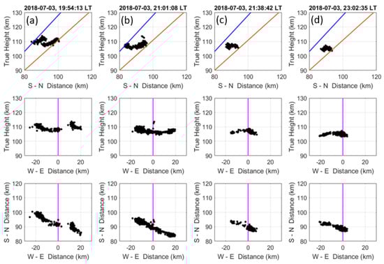
Figure 9.
Selected examples of the spatial structures of the Es layers severely modulated by the gravity waves, in which concave (cases (a,b)) and convex (cases (c,d)) modulations are clearly seen. The height amplitudes of the wave modulations are about 5 km, 5.5 km, 3 km, and 4 km for cases (a–d), respectively.
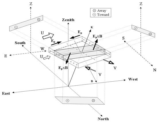
Figure 10.
Schematic model showing generation of polarized electric field Ep in a tilted Es layer modulated by a gravity wave, in which k is the radar wave vector perpendicular to the local magnetic field line B, U represents zonal wind of background semi-diurnal tide, and V is the meridional wind velocity of the gravity wave. As shown, eastward (westward) Ep is generated in the western (eastern) part of the Es layer. Because of the Ep × B drift effect, the former will be higher than the latter, and a tilted Es plasma structure is formed.
From the radar-observed Doppler velocities of the gravity-wave-associated 3 m FAI echoes, we can estimate the polarized electric fields that drive the 3 m FAIs to move through the E × B drift effect. As shown in Figure 4, the magnitudes of Doppler velocities of the 3 m FAI echoes are in a range between −95 m/s and 86 m/s, corresponding to zonally pointed polarized electric fields embedded in the Es layer with a range from −3.0 mV/m westward to 3.3 mV/m eastward. These values are basically in agreement with other measurements [,].
4. Discussion and Conclusions
There is mounting evidence that a horizontally stratified Es layer will be modulated when a vertically propagating gravity wave interacts with the Es layer (e.g., Huang and Kelley []; Yokoyama et al. []). The height modulation of the Es layer caused by propagating gravity waves has been numerically investigated. Huang and Kelley [] suggested that the Es layer can be modulated about 10 km in height by the gravity wave. The simulation result obtained by Yokoyama et al. [] showed that about 2–5 km height modulation of the Es layer could be achieved by the polarization electric field generated by a gravity wave propagating in the meridional direction. Bernhardt [] theoretically investigated Es layer modulation by using Kelvin–Helmholtz instability associated with a horizontally propagating gravity wave with a horizontal wavelength of about 8.8 km to account for the modulation of the Es layer. Bernhardt [] found that the Es layer could be modulated in height only about 0.5 to 1.5 km by gravity-wave-associated K-H billows, and the width of the layer across the K-H billow axis is about a few kilometers. Chu and Yang [], using interferometry measurement, measured height modulation of 0.3–1.2 km. In this study, Figure 6 and Figure 9 demonstrate observational evidence that the height of the Es layer modulated by the sharply steepened gravity wave can be as large as 10 km or more, supporting the results obtained by Huang and Kelley []. In addition, as shown in the upper panels of Figure 4 and Figure 5, there are salient downward movements of the phase fronts of the FAI Doppler velocities and echo intensities for the time intervals of 20:53–21:02, 21:05–21:32, and 22:04–22:21 LT. These features are also indications of the upward propagations of the atmospheric gravity waves in the Es layer [,].
In Figure 4 and Figure 5, it is evident that, during the time interval when the propagations of the gravity wave were prevailing, the Doppler velocities of the FAI echoes were characterized as positive in the upper part of the Es layer and negative in the bottom side of the Es layer. The maximum vertical Doppler velocity shear can be as large as 68 m/s/km or more at times 20:57 LT and 21:02 LT. There is a tendency for the velocity shears to descend with the background Es layer, especially for the FAI echoes during the periods when the echo bulges were present. These features, combined with the horizontal distributions of the Doppler velocity shears that occurred quasi-periodically, strongly suggest that the prominent Doppler velocity shears bear close relation to the dynamic structures of the gravity wave. In order to explore the relations between the propagation of the gravity wave and the distribution of the Doppler velocity shear mentioned above, a schematic model is proposed below. Figure 10 is a schematic model of a background Es layer that is subjected to the effects of vertical wind shear of the zonal wind component U of a background tidal wind and the gravity-wave-induced meridional wind component V. The former is responsible for the formation of the thin Es layer, and the latter generates the polarized electric field Ep in the Es layer to drive the FAIs to drift in the direction perpendicular to the local magnetic field lines. The shaded parallelepiped is the radar-observed echoing region from the Es FAIs, which is the region where the radar wave vector K is nearly perpendicular to the local magnetic field lines B with an aspect angle usually less than 0.2°. The shaded parallelograms are, respectively, the projections of the echoing region on the vertical plane (with N-S and vertical axes), zonal pane (with E-W and vertical axes), and horizontal plane (with N-S and E-W axes). It is important to note that the radar-observed Doppler velocity of the Es FAIs is essentially the Ep × B drift velocity of the free electron in the Es layer. In the context of the Es layer shown in Figure 10, the west end of the radar-observed echoing region is expected to be higher than that at the east end due to the Ep × B drift effect that tends to lift up the west end and lower down the east end of the Es layer. As a result, a tilted Es layer is formed, and the positive Doppler velocity of the Es FAI echoes will be present in the upper portion of the tilted Es layer projected on the vertical plane, and the negative Doppler velocity will occur in the lower part of the projected echoing region. As for the FAI echoing regions projected on the zonal plane, it is obvious that the FAI echoes will be higher at the west end than those at the east end. Therefore, the schematic model proposed in Figure 10 can essentially account for the distributions of the radar-observed FAI echoes shown in Figure 4.
In summary, the response of a background thin Es layer with a thickness of 2–4 km that was formed by a semi-diurnal tide in a height range of 100–120 km through wind shear convergence process to upward propagating gravity waves is investigated in this article. We find that the Es layer was severely disturbed and modulated by the gravity wave with a dominant wave period of 46.3 min to generate large-scale plasma irregularities with dimensions in ranges of about 4–12 km, 10–28 km, and 6–14 km in the vertical, zonal, and meridional directions, respectively. The vertical, zonal, and true meridional drift velocity components of the plasma structures, which are estimated from the displacement of echo patterns projected on the three mutually orthogonal planes, were approximately in the range of −15–16 m/s, −91–50 m/s, and −13–26 m/s, respectively. These features strongly indicate modulations of the Es layer location and FAIs movement made by upward and horizontally propagating inertial gravity waves. Evidence is provided that the waves were propagating predominantly from east-southeast to west-northwest at a phase velocity of about 16 m/s and propagation direction of about 16.5° with respect to the westward direction.
Author Contributions
Conceptualization, Y.-H.C. and C.M.S.; methodology, Y.-H.C. and C.M.S.; software, Y.-H.C., C.M.S. and C.-Y.W.; validation, Y.-H.C., C.M.S., C.-L.S. and C.-Y.W.; formal analysis, Y.-H.C. and C.M.S.; investigation, Y.-H.C. and C.M.S.; resources, Y.-H.C. and C.-L.S.; data curation, Y.-H.C. and C.M.S.; writing—original draft preparation, Y.-H.C.; writing—review and editing, Y.-H.C. and C.M.S.; visualization, Y.-H.C. and C.M.S.; supervision, Y.-H.C.; project administration, Y.-H.C. and C.-L.S.; funding acquisition, Y.-H.C. All authors have read and agreed to the published version of the manuscript.
Funding
This research was funded by Ministry of Science and Technology, under grants MOST 109-2111-M-008-024.
Institutional Review Board Statement
Not applicable.
Informed Consent Statement
Not applicable.
Data Availability Statement
Data sharing is not applicable to this article.
Acknowledgments
The Chung-Li VHF radar is operated and maintained by the Department of Space Science and Engineering, National Central University, Taiwan, the Republic of China (ROC). The VHF radar data are obtainable by contacting the authors or the Chung-Li radar site (yhchu@jupiter.ss.ncu.deu.tw).
Conflicts of Interest
The authors declare no conflict of interest.
References
- Cai, X.; Yuan, T.; Eccles, J.V.; Raizada, S. Investigation on the distinct nocturnal secondary sodium layer behavior above 95 km in winter and summer over Logan, UT (41.7° N, 112° W) and Arecibo Observatory, PR (18.3° N, 67° W). J. Geophys. Res. Space Phys. 2019, 124, 9610–9625. [Google Scholar] [CrossRef]
- Yuan, T.; Wang, J.; Cai, X.; Sojka, J.; Rice, D.; Oberheide, J.; Criddle, N. Investigation of the seasonal and local time variations of the high-altitude sporadic Na layer (Nas) formation and the associated midlatitude descending E layer (Es) in lower E region. J. Geophys. Res. Space Phys. 2014, 119, 5985–5999. [Google Scholar] [CrossRef]
- Delgado, R.; Friedman, J.S.; Fentzke, J.T.; Raizada, S.; Tepley, C.A.; Zhou, Q. Sporadic metal atom and ion layers and their connection to chemistry and thermal structure in the mesopause region at Arecibo. J. Atmos. Sol.-Terr. Phys. 2012, 74, 11–23. [Google Scholar] [CrossRef]
- Dou, X.K.; Xue, X.H.; Li, T.; Chen, T.D.; Chen, C.; Qiu, S.C. Possible relations between meteors, enhanced electron density layers, and sporadic sodium layers. J. Geophys. Res. 2010, 115, A06311. [Google Scholar] [CrossRef]
- Calvert, W.; Warnock, J.M. Ionospheric irregularities observed by topside sounders. Proc. IEEE 1969, 57, 1019–1025. [Google Scholar] [CrossRef]
- Morse, F.A.; Edgar, B.C.; Koons, H.C.; Rice, C.J.; Heikkila, W.J.; Hoffman, J.H.; Tinsley, B.A.; Winningham, J.D.; Christensen, A.B.; Woodman, R.F.; et al. Equion, an equatorial ionospheric irregularity experiment. J. Geophys. Res. Atmos. 1977, 82, 578–592. [Google Scholar] [CrossRef]
- Fejer, B.G.; Kelley, M.C. Ionospheric irregularities. Rev. Geophys. 1980, 18, 401–454. [Google Scholar] [CrossRef]
- Yamamoto, M.; Fukao, S.; Woodman, R.F.; Ogawa, T.; Tsuda, T.; Kato, S. Midlatitude E region field-aligned irregularities observed with the MU radar. J. Geophys. Res. 1991, 96, 15943–15949. [Google Scholar] [CrossRef]
- Fritts, D.C.; Abdu, M.A.; Batista, B.R.; Batista, I.S.; Batista, P.P.; Buriti, R.; Clemesha, B.R.; Dautermann, T.; de Paula, E.R.; Fechine, B.J.; et al. Overview and summary of the Spread F Experiment (SpreadFEx). Ann. Geophys. 2009, 27, 2141–2155. [Google Scholar] [CrossRef]
- Chu, Y.H.; Brahmanandam, P.S.; Wang, C.Y.; Su, C.L.; Kuong, R.M. Coordinated sporadic E layer observations made with Chung-Li 30 MHz radar, ionosonde and FORMOSAT3/COSMIC satellites. J. Atmos. Sol.-Terr. Phys. 2011, 73, 883–894. [Google Scholar] [CrossRef]
- Chen, G.; Wu, C.; Zhao, Z.; Zhong, D.; Qi, H.; Jin, H. Daytime E region field-aligned irregularities observed during a solar eclipse. J. Geophys. Res. Space Phys. 2015, 119, 10633–10640. [Google Scholar] [CrossRef]
- Farley, D.T. A theory of electrostatic field in a horizontally stratified ionosphere subject to a vertical magnetic field. J. Geophys. Res. 1959, 64, 1225–1233. [Google Scholar] [CrossRef]
- Farley, D.T. Theory of equatorial electrojet plasma waves: New developments and current status. J. Atmos. Terr. Phys. 1985, 47, 729–744. [Google Scholar] [CrossRef]
- Fejer, B.G.; Providakes, J.; Farley, D.T. Theory of plasma waves in the auroral E region. J. Geophys. Res. 1984, 89, 7487–7494. [Google Scholar] [CrossRef]
- Gurevich, A.V.; Borisov, N.D.; Zybin, K.P. Ionospheric turbulence induced in the lower part of the E region by the turbulence of the neutral atmosphere. J. Geophys. Res. 1997, 102, 379–388. [Google Scholar] [CrossRef]
- Wang, C.-Y.; Chu, Y.-H.; Su, C.-L.; Kuong, R.-M.; Chen, H.-C.; Yang, K.-F. Statistical investigations of layer-type and clump-type plasma structures of 3-m field-aligned irregularities in nighttime sporadic E region made with Chung-Li VHF radar. J. Geophys. Res. 2011, 116, A12311. [Google Scholar] [CrossRef]
- Axford, W.I. The formation and vertical movement of dense ionized layers in the ionosphere due to neutral windshears. J. Geophys. Res. 1963, 68, 769–779. [Google Scholar] [CrossRef]
- Whitehead, J.D. Recent work on mid-latitude and equatorial sporadic-E. J. Atmos. Terr. Phys. 1989, 51, 401–424. [Google Scholar] [CrossRef]
- Chu, Y.H.; Wang, C.Y.; Wu, K.H.; Chen, K.T.; Tzeng, K.J.; Su, C.L.; Feng, W.; Plane, J.M.C. Morphology of sporadic E layer retrieved from COSMIC GPS radio occultation measurements: Wind shear theory examination. J. Geophys. Res. Space Phys. 2014, 119, 2117–2136. [Google Scholar] [CrossRef]
- Sudan, R.N. Unified theory of type-I and type-II irregularities in the equatorial electrojet. J. Geophys. Res. 1983, 88, 4853–4860. [Google Scholar] [CrossRef]
- Providakes, J.; Farley, D.T.; Fejer, B.G.; Sahr, J.; Swartz, W.E.; Hxggstrbm, I.; Hedberg, A.; Nordling, J.A. Observations of aurora1 E-region plasma waves and electron beating with EISCAT and a VHF radar interferometer. J. Atmos. Terr. Phys. 1988, 50, 339–356. [Google Scholar] [CrossRef]
- Sahr, J.D.; Farley, D.T.; Swartz, W.E.; Providakes, J.F. The altitude of type 3 auroral irregularities: Radar interferometer observations and implications. J. Geophys. Res. 1991, 96, 17805–17811. [Google Scholar] [CrossRef]
- Tsunoda, R.T. On blanketing sporadic E and polarization effects near the equatorial electrojet. J. Geophys. Res. 2008, 113, A09304. [Google Scholar] [CrossRef]
- Clemesha, B.R. Sporadic neutral metal layers in the mesosphere and lower thermosphere. J. Atmos. Terr. Phys. 1995, 57, 725–736. [Google Scholar] [CrossRef]
- MacDougall, J.W.; Plane, J.M.; Jayachandran, P.T. Polar cap Sporadic E: Part 2, modeling. J. Atmos. Sol.-Terr. Phys. 2000, 62, 1169–1176. [Google Scholar] [CrossRef]
- Lu, F.; Farley, D.T.; Swartz, W.E. Spread in aspect angles of equatorial E region irregularities. J. Geophys. Res. 2008, 113, A11309. [Google Scholar] [CrossRef]
- Chu, Y.H.; Yang, K.F.; Wang, C.Y.; Su, C.L. Meridional electric fields in layer-type and clump-type plasma structures in midlatitude sporadic E region: Observations and plausible mechanisms. J. Geophys. Res. Space Phys. 2013, 118, 1243–1254. [Google Scholar] [CrossRef]
- Farley, D.T.; Ierkie, H.M.; Fejer, B.G. Radar interferometry: A new technique for studying plasma turbulence in the ionosphere. J. Geophys. Res. 1981, 86, 1467–1472. [Google Scholar] [CrossRef]
- Chu, Y.H.; Wang, C.Y. Interferometry observations of three-dimensional spatial structures of sporadic E irregularities using the Chung-Li VHF radar. Radio Sci. 1997, 32, 817–832. [Google Scholar] [CrossRef]
- Van Eyken, A.P.; Williams, P.J.S.; Maude, A.D.; Morgan, G. Atmospheric gravity waves and sporadic-E. J. Atmos. Terr. Phys. 1982, 44, 25–29. [Google Scholar] [CrossRef]
- Bourdillon, A.; Lefur, E.; Haldoupis, C.; Le Roux, Y.; MeÂnard, J.; Delloue, J. Decameter mid-latitude sporadic-E irregularities in relation with gravity waves. Ann. Geophysicae 1997, 15, 925–934. [Google Scholar] [CrossRef]
- Patra, A.K.; Rao, N.V.; Choudhary, R.K. Daytime low-altitude quasi-periodic echoes at Gadanki: Understanding of their generation mechanism in the light of their Doppler characteristics. Geophys. Res. Lett. 2009, 36, L05107. [Google Scholar] [CrossRef]
- Woodman, R.F.; Yamamoto, M.; Fukao, S. Gravity wave modulation of gradient drift instabilities in mid-latitude sporadic E irregularities. Geophys. Res. Lett. 1991, 18, 1197–1200. [Google Scholar] [CrossRef]
- Hysell, D.L.; Yamamoto, M.; Fukao, S. Imaging radar observations and theory of type I and type II quasi-periodic echoes. J. Geophys. Res. 2002, 107, 1360. [Google Scholar] [CrossRef]
- Maruyama, T.; Saito, S.; Yamamoto, M.; Fukao, S. Simultaneous observation of sporadic E with a rapid-run ionosonde and VHF coherent backscatter radar. Ann. Geophysicae 2006, 24, 153–162. [Google Scholar] [CrossRef]
- Chu, Y.H.; Wang, C.Y.; Yang, K.F. Plasma structures responsible for sporadic E region quasi-periodic echoes. J. Atmos. Sol. -Terr. Phys. 2007, 69, 537–551. [Google Scholar] [CrossRef]
- Tanaka, T.; Venkateswaran, S.V. Characteristics of field aligned E-region irregularities over Ioka (36o), Japan, I. J. Atmos. Terr. Phys. 1982, 44, 381–394. [Google Scholar] [CrossRef]
- Riggin, D.; Swartz, W.E.; Providakes, J.; Farly, D.T. Radar studies of long-wavelength waves associated with midlatitude sporadic E layers. J. Geophys. Res. 1986, 91, 8011–8024. [Google Scholar] [CrossRef]
- Yamamoto, M.; Komoda, N.; Fukao, S.; Tsunoda, R.T.; Ogawa, T.; Tsuda, T. Spatial structure of the E-region field aligned irregularities revealed by the MU radar. Radio Sci. 1994, 29, 337–347. [Google Scholar] [CrossRef]
- Wang, C.Y.; Chu, Y.H. Interferometry investigations of blob-like sporadic E plasma irregularity using the ChungLi VHF radar. J. Atmos. Sol.-Terr. Phys. 2001, 63, 123–133. [Google Scholar] [CrossRef]
- Chu, Y.H.; Wang, C.Y. Interferometry investigations of VHF backscatter from plasma irregularity patches in the nighttime E region using the Chung-Li radar. J. Geophys. Res. 1999, 104, 2621–2631. [Google Scholar] [CrossRef]
- Chu, Y.-H.; Wang, C.-Y. Plasma structures of 3meter type 1 and type 2 irregularities in nighttime midlatitude sporadic E region. J. Geophys. Res. 2002, 107, 1447. [Google Scholar]
- Saito, S.; Yamamoto, M.; Hashiguchi, H.; Maegawa, A.; Saito, A. Observational evidence of coupling between quasiperiodic echoes and mediumscale traveling ionospheric disturbances. Ann. Geophys. 2007, 25, 2185–2194. [Google Scholar] [CrossRef]
- Lin, T.-H.; Chu, Y.-H.; Su, C.-L.; Yang, K.-F. Radar phase offset estimate using ionospheric field-aligned irregularities and aircraft. Terr. Atmos. Ocean. Sci. 2019, 30, 803–820. [Google Scholar] [CrossRef]
- Chu, Y.-H.; Wang, C.-Y. Radial velocity and doppler spectral width of echoes from field-aligned irregularities localized in the sporadic E region. J. Geophys. Res. 2003, 108, 1282. [Google Scholar] [CrossRef]
- Chu, Y.H.; Wang, C.Y. An evidence of beam broadening effect dominating Doppler spectra of field-aligned irregularities in sporadic E region made with the Chung-Li radar. J. Geophys. Res. 2005, 110, A09305. [Google Scholar] [CrossRef]
- Arras, C.; Jacobi, C.; Wickert, J. Semidiurnal tidal signature in sporadic E occurrence rates derived from GPS radio occultation measurements at higher midlatitudes. Ann. Geophys. 2009, 27, 2555–2563. [Google Scholar] [CrossRef]
- Tsai, L.-C.; Su, S.-Y.; Liu, C.-H.; Schuh, H.; Wickert, J.; Alizadeh, M.M. Global morphology of ionospheric sporadic E layer from the FormoSat-3/COSMIC GPS radio occultation experiment. GPS Solut. 2018, 22, 118. [Google Scholar] [CrossRef]
- Kelley, M.C. The Earth’s Ionosphere; Academic Press: San Diego, CA, USA, 1989. [Google Scholar]
- Gossard, E.E.; Hooke, W.H. Waves in the Atmosphere; Elsevier: New York, NY, USA, 1975. [Google Scholar]
- Chu, Y.H.; Su, C.L.; Larsen, M.F.; Chao, C.K. First measurements of neutral wind and turbulence in the mesosphere and lower thermosphere over Taiwan with a chemical release experiment. J. Geophys. Res. 2007, 112, A02301. [Google Scholar] [CrossRef]
- Gelinas, L.J.; Kelley, M.C.; Larsen, M.F. Large-scale E-region electric field structure due to gravity wave winds. J. Atmos. Solar Terr. Phys. 2002, 64, 1465–1469. [Google Scholar] [CrossRef]
- Huang, C.S.; Kelley, M.C. Numerical simulations of gravity wave modulation of midlatitude sporadic E layers. J. Geophys. Res. 1996, 101, 24533–24543. [Google Scholar] [CrossRef]
- Yokoyama, T.; Yamamoto, M.; Fukao, S. Computer simulation of polarization electric fields as a source of midlatitude field-aligned irregularities. J. Geophys. Res. 2003, 108, 1054. [Google Scholar] [CrossRef]
- Bernhardt, P. The modulation of sporadic E layers by Kelvin-Helmholtz billows in the neutral atmosphere. J. Atmos. Sol. Terr. Phys. 2002, 105, 1487–1504. [Google Scholar] [CrossRef]
- Chu, Y.H.; Yang, K.F. Reconstruction of spatial structure of thin layer in sporadic E region by using VHF coherent scatter radar. Radio Sci. 2009, 44, RS5003. [Google Scholar] [CrossRef]
Disclaimer/Publisher’s Note: The statements, opinions and data contained in all publications are solely those of the individual author(s) and contributor(s) and not of MDPI and/or the editor(s). MDPI and/or the editor(s) disclaim responsibility for any injury to people or property resulting from any ideas, methods, instructions or products referred to in the content. |
© 2023 by the authors. Licensee MDPI, Basel, Switzerland. This article is an open access article distributed under the terms and conditions of the Creative Commons Attribution (CC BY) license (https://creativecommons.org/licenses/by/4.0/).