Increasing NH₃ Emissions in High Emission Seasons and Its Spatiotemporal Evolution Characteristics during 1850–2060

Abstract

Ammonia (NH₃) is a crucial alkaline component in the atmosphere, with significant impacts on environmental and ecosystem health. However, our understanding of the long-term variability characteristics of NH₃ emissions is still limited due to the scarcity of long-term continuous NH₃ emission observation data. In this study, we investigated the global NH₃ emission evolution pattern during the high-emission season (March–August) in historical (1850–2014) and future (2015–2060) periods, based on the simulated global NH₃ emission and temperature data using the CESM2-WACCM model from CMIP6. We utilized cluster analysis, KNN regression simulation, and transfer matrix analysis to explore the emission characteristics. In the historical period, the analysis revealed that the high NH₃ emission season is March–August, accounting for about 60% of annual emissions, with a significant increasing trend of NH₃ emissions. The global average NH₃ emissions in the last 164 years were about four times higher (28.06 mg m⁻²) than those in 1850 (5.52 mg m⁻²). Moreover, on the intercontinental scale, NH₃ emissions from 1850 to 2014 March–August exhibited dynamic increases characterized differently across continents. Europe showed an increasing and then decreasing trend, Asia demonstrated a rapid increase, while South America, North America, and Africa exhibited medium increases, and Australia showed low increases. The global NH₃ emissions experienced three distinct periods of low (1850–1964, slope = 0.059 mg m⁻² y⁻¹), high (1965–1988, slope = 0.389 mg m⁻² y⁻¹), and medium (1989–2014, slope = 0.180 mg m⁻² y⁻¹) rates of increase. Starting from the high rate of increase period, the hotspots of global NH₃ emissions gradually shifted from Europe to East and South Asia. Looking ahead, our findings suggest that the global NH₃ emission rate will tend to slow down under the Representative Concentration Pathway (RCP) 4.5 and RCP8.5 warming scenarios. However, compared with the medium-rate increasing period, the moderate and heavy NH₃ emission areas under RCP4.5 and RCP8.5 scenarios will show a tendency to expand by 2060, with the proportion of area covered by heavy emissions increasing by 0.55% and 0.56%, respectively. In conclusion, our study highlights that NH₃ pollution remains a significant environmental challenge in the future period, with Asia and Europe being the key areas requiring attention for NH₃ emission reduction.

1. Introduction

Ammonia (NH₃) is a vital constituent of the global nitrogen cycle and the most abundant alkaline compound in the atmosphere [1,2]. It serves as a precursor to secondary inorganic aerosols that react with atmospheric sulfuric acid and nitrate. This reaction results in the formation of particulate matter, including ammonium sulfate and ammonium nitrate, leading to an increase in PM_2.5 concentration and adversely impacting air quality [3]. For instance, in certain densely populated areas of Europe, the contribution of secondary atmospheric NH₃ salt aerosol particulate matter accounts for 10–20% of the local PM_2.5 mass concentration [4]. For humans and animals, high concentrations of NH₃ pairs are toxic not only to the brain, but they may also cause adverse symptoms such as eye damage, respiratory inflammation, and mucosal hemorrhage [5,6,7]. Additionally, gaseous NH₃ and particulate ammonium salts can also cause a decrease in plant photosynthetic rate and biodiversity when they settle to the surface, as well as the eutrophication of lakes or offshore waters and soil acidification [8,9]. In recent decades, significant research efforts have been dedicated to the control of pollutants such as SO₂ and NO_x, while NH₃ pollution has received comparatively less attention [10]. Moreover, as the reduction in SO₂ and NO_x progresses, NH₃ pollution has the potential to become increasingly serious [11,12]. However, controlling NH₃ emissions during winter has been found to be more effective in reducing PM_2.5 mass concentrations compared to controlling SO₂ and NO_x [13]. Additionally, the marginal cost of NH₃ emission reduction is significantly lower, representing only 10% of the cost associated with NO_x [3], thereby making it a more feasible option [14]. Gaining a comprehensive understanding of the long-term trends, as well as the spatial and temporal evolution of atmospheric NH₃ emissions, is imperative for the effective management of NH₃ pollution in the future, and for enhancing the global ecological environment.

Currently, ammonia emissions originating from fertilizer application in agricultural activities and livestock manure in animal husbandry account for more than 57% of global ammonia emissions, establishing them as the primary anthropogenic source of atmospheric ammonia emissions [15,16]. Furthermore, NH₃ volatilization can also occur due to industrial production, vehicle emissions, and biomass burning [17,18]. The global population has been steadily increasing, resulting in a growing demand for food and meat, which has subsequently led to a significant rise in nitrogen fertilizer application and livestock farming in recent years [19,20]. A study has revealed that global NH₃ emissions from agricultural and livestock development underwent a substantial 78% increase between 1980 and 2018 [21]. It has been observed that global ammonia emissions have exhibited a distinct upward trend in recent decades. The EDGAR emission model reports a 20% increase in overall ammonia emissions from 2000 to 2010 [22], while the Infrared Atmospheric Sounding Interferometer (IASI) has documented a 12.8 ± 1.3% increase in overall ammonia emissions from 2008 to 2018 [23]. Nevertheless, significant regional disparities exist in the spatial distribution of global ammonia emissions [23]. For instance, NH₃ emissions in China have surged approximately 2.4 times between 1980 and 2016, and it is anticipated that this trend will persist unless emission reduction policies are implemented by 2030 [24]. The Indo-Gangetic Plain (IGP) stands out as one of the largest and fastest-growing regions contributing to global NH₃ emissions, with a summer annual growth rate of 1.2% observed between 2008 and 2016 [25]. Additionally, it has been observed that the seasonality of ammonia emissions varies across regions due to differences in the primary sources of emissions and meteorological conditions [26]. A study investigating monthly ammonia emissions in the United States from 2008 to 2017 demonstrated that the overall concentration of emissions was primarily observed during the spring and summer months, with peak values occurring in July and August in the western region, and in May and June in the eastern region [27]. Nonetheless, comprehensive examinations of the spatial and temporal dynamics of global NH₃ emissions on a large scale remain limited, with a lack of understanding regarding their spatial and temporal evolution over a century-long period. This knowledge gap impedes the scientific management of NH₃ pollution within the context of global warming in the future.

This study aims to analyze the spatial and temporal dynamics of global NH₃ emissions from 1850 to 2014 using historical simulation data from the CESM2-WACCM model in CMIP6. Additionally, it seeks to predict future emissions from 2015 to 2060 under various warming scenarios using the KNN regression model. The outcomes of this study are anticipated to offer a scientific foundation for the implementation of effective measures aimed at reducing and managing NH₃ emissions.

2. Data and Methods

2.1. NH₃ Emission Data

To analyze the long-term trends and characteristics of the spatial and temporal evolution of global NH₃ emissions, we utilized historical NH₃ emission simulation data generated by the CESM2-WACCM model in CMIP6, which was obtained from the website https://esgf-node.llnl.gov/search/cmip6/ (accessed on 21 January 2022). This dataset provides NH₃ emission rate data from January 1850 to December 2014, with a spatial resolution of 0.9375° × 1.25° and a temporal resolution of months. The simulated atmospheric pollution data from the CESM2-WACCM model align with the variability patterns observed in ground-based O₃ and PM_2.5 data during the historical period [28]. It has been observed that NH₃ is strongly correlated with increased atmospheric PM_2.5 levels [29,30]. Additionally, the CESM2-WACCM model demonstrates good performance in simulating surface energy fluxes across global continents [31], and has been widely used in the study of various air pollutants [32].

2.2. Temperature Data

We used temperature data from the CRUTS (Climatic Research Unit gridded Time Series) dataset, covering the period from 1901 to 2014, in order to examine the correlation between NH₃ emissions and temperature. We obtained the data from the website https://crudata.uea.ac.uk/cru/data/hrg/cru_ts_4.05/cruts.2103051243.v4.05/tmp/ (accessed on 9 August 2022). They possessed a spatial resolution of 0.5° × 0.5° and a temporal resolution at the monthly level. To evaluate the effect of future warming on NH₃ emissions, we employed the monthly average temperature data obtained from the Representative Concentration Pathway (RCP) 4.5 and RCP8.5 experiments conducted with the Earth System Model MPI-ESM-LR at the German Max Planck Institute for Meteorology within CMIP5 (https://esgf-node.llnl.gov/search/cmip5/, accessed on 29 August 2022). These datasets cover the time period from 2015 to 2060 and have a spatial resolution of 1.875° × 1.875°. RCP4.5 represents a medium emissions scenario where global temperatures are expected to increase by approximately 1.8 °C by 2100 compared to pre-industrial levels. RCP8.5 represents a high emissions scenario where the temperature increase is projected to be around 3.7 °C. We interpolated the temperature data onto a grid with a spatial resolution of 0.9375° × 1.25° using a bilinear interpolation method.

2.3. Time-Series Feature Extraction Based on Bottom-Up Algorithm

We employed the bottom-up algorithm to partition the linear representation of NH₃ emission time series from 1850 to 2014 into segments for analyzing its time-series dynamics. The bottom-up algorithm is a data-mining technique that enhances effectiveness by classifying similar data into segments [33]. Initially, the algorithm divides the original sequence linearly based on all the data points within it, resulting in an initial segmented linear representation with a fit error of zero. Next, the algorithm calculates the merging cost between each linear segment and its adjacent segments. Subsequently, it merges adjacent linear segments sequentially based on the smallest merging cost and repeats this process until preset conditions are met.

2.4. NH₃ Emission Prediction Based on KNN Regression Model

Previous research has demonstrated a significant correlation between temperature and NH₃ emissions, which affects both their spatial distribution and emission levels [34]. In order to investigate the impact of future climate change scenarios (RCP4.5 and RCP8.5) on the spatial and temporal patterns of NH₃ emissions, we constructed a KNN (K-Nearest Neighbor) regression model for temperature–NH₃. This model was used to simulate and analyze the spatial and temporal characteristics of global NH₃ emissions for the period 2015–2060 under RCP45 and RCP85. The KNN algorithm is commonly used in time series forecasting, as it is not only simple to implement, but also provides clear prediction results [35]. The KNN regression algorithm consists of the following steps:

• The training set $X_i=\left(x_i^1,x_i^2,\dots ,x_i^n,y_i\right)$, where $i=1,2,\dots ,n$. Let a point of the test set be $X=\left(x_1,x_2,\dots ,x_n,y\right)$;
• Compute the Euclidean distance $L$ between each point $X_i$ in the training set and a point X in the training set:

  $$L\left(X,X_i\right)=\sqrt{{\displaystyle \sum }_{m=1}^n{\left(x_m-x_i^m\right)}^2}$$

  (1)
• Sort the distances $L$ by size and select the $k$ nearest neighbors $X_j\left(1\le j\le k\right)$ in the training set with $X$. Find the average value of these $k$ nearest neighbors and use it as the output prediction of $X$ $\widehat{\mathrm{y}}$, i.e.,

  $$\widehat{\mathrm{y}}={\displaystyle \sum }_{\mathrm{j}=1}^{\mathrm{k}}{\mathrm{y}}_{\mathrm{j}}/\mathrm{k}$$

  (2)

In our study, we utilized annual average CMIP6-based observations of NH₃ emissions from March to August 1965 to 2014 as the dependent variable (y) and temperature observations from CRUTS as the independent variable (x) for constructing a KNN regression model. For model construction, we randomly selected 20% of the data as the test set and the remaining 80% of the data as the training set. The come hyperparameter automatic optimization method was employed for training the optimization model. Based on the results, at k = 4 (k being the number of reference neighbor label values), the prediction effect was optimal. The optimized KNN model can predict NH₃ emissions more accurately. We found that the simulation results were significantly positively correlated with the number of tests (n = 50, R² = 0.66, p < 0.001), and the RMSE (root mean square error) of both was small (23.42 mg m⁻²).

2.5. Spatial Feature Identification of NH₃ Emission Based on K-Means Algorithm

To compare the extent of NH₃ emissions across different regions of the world, we used the K-Means clustering algorithm. This unsupervised clustering algorithm requires several iterations to classify NH₃ emissions in each region into three categories based on their size: light, moderate, and heavy emissions. The training process involves calculating the Euclidean distance between samples in the dataset to analyze their similarity. The data with closer Euclidean distance between sample points and the center point are then clustered into one cluster. Afterward, different clusters with higher overall differences are divided into different classes based on a comparison of overall differences between them. This method has been widely used in studies to cluster various pollutants [36,37].

2.6. Spatial and Temporal Transfer of NH₃ Emissions Based on Transfer Matrix

To analyze how global NH₃ emissions change over time and space, we used Markov transfer matrices. This method allows us to calculate the changes in transfer between different levels of NH₃ emissions in adjacent time periods. Markov transfer matrix analysis is a technique based on Markov chain theory, which calculates the probability of transferring matrix elements from one state to another during time series changes [38]. This approach has been widely used to investigate changes in the spatial and temporal dynamics of the transfer of environmental elements, and can help visualize the direction of the transfer and the changes in the spatial pattern of environmental elements [39]. The formula for Markov transfer matrices is as follows:

$$S_{ij}=\left[\begin{array}{ccc}{S}_{11}& S_{12}& S_{13}\\ S_{21}& S_{22}& S_{23}\\ S_{31}& S_{32}& S_{33}\end{array}\right]$$

(3)

In the equation, i and j (i, j = 1, 2, 3) represent the initial and final levels of NH₃ emissions, respectively; $S_{ij}$ represents the area where the initial level i of NH₃ emissions is transferred to the final level j of NH₃ emissions.

3. Results

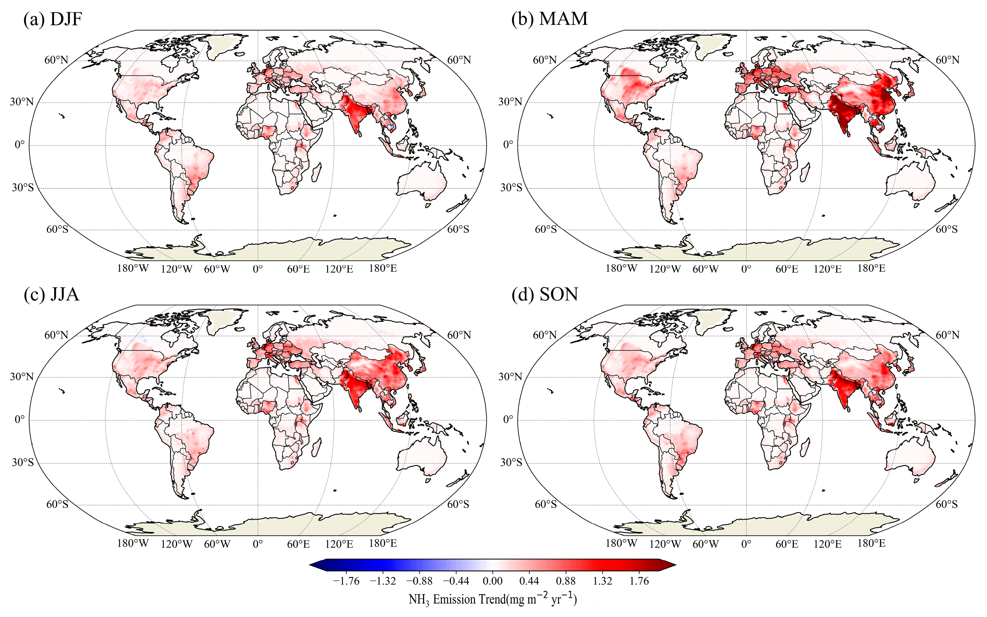
3.1. Seasonal Variation Characteristics of Global NH₃ Emissions during Historical Periods

As shown in Figure 1, we analyzed the annual variation rates of NH₃ emissions in each season from 1850 to 2014 and investigated the seasonal variation characteristics of NH₃ emissions in each region of the world. The results reveal a consistent upward trend in NH₃ emissions across all seasons and regions worldwide over the 165-year period. However, there were minor decreases observed in individual regions of South Asia. The most substantial increases in NH₃ emissions were primarily concentrated in the spring and summer seasons.

The regions experiencing the highest growth rates of emissions are predominantly concentrated in the Netherlands, Belgium, the North China Plain, India, and Pakistan. The Netherlands and Belgium, which have the fastest overall growth rates, exhibited similar growth rates in the spring, around 1.50 mg m⁻² y⁻¹. The most significant growth was observed in the North China Plain during the spring, where the fastest growing areas experienced rates of up to 8.50 mg m⁻² y⁻¹, consistent with the findings of previous studies [32]. Pakistan and the Ganges Plain of India make significant contributions to NH₃ emissions in South Asia, with an extremely rapid increase observed during the spring for the entire region, with a growth rate of 0.868 mg m⁻² y⁻¹. Additionally, faster increases were observed in other European countries and regions, such as south-central North America, with an overall growth rate of 0.14 mg m⁻² y⁻¹ for the European region. The growth patterns of these regions were relatively similar, exhibiting greater uniformity seasonally, but with a significant increase during the spring. Both Africa and South America also showed a positive trend in the increase, but with smaller growth rates, with most regions exhibiting an increase rate of 0.44 mg m⁻² yr⁻¹ or less. However, we observed a slight decrease in NH₃ emissions during the winter in the northern part of Cambodia in Southeast Asia, with a rate of 0.91 mg m⁻² y⁻¹, possibly attributable to a decrease in local biomass burning activities [23].

We conducted a statistical analysis on the proportion of total NH₃ emissions within the annual emissions for all seasons from 1850 to 2014. As illustrated in Figure 2, global NH₃ emissions are concentrated in two time periods, MAM and JJA, which can account for up to 60% of the annual emissions, while the respective shares of SON and DJF never exceed 25%. In the early stages, the highest proportion was observed in JJA, and this gradually shifted towards MAM over time. Around 1920, the proportion of MAM became equal to that of JJA and subsequently surpassed it, thus becoming the season with the largest proportion. This may be attributed to the fact that NH₃ emissions are primarily caused by agricultural fertilizer application and livestock manure. Initially, before the widespread use of chemical fertilizers, animal manure was the primary source of NH₃ emissions, with summer being the peak season for emissions. However, with the widespread use of chemical fertilizers, NH₃ emissions increased in areas with intensive fertilizer-dependent agriculture [40], with spring gradually surpassing summer. In light of these analyses, this paper will focus on the MAM-JJA period, which exhibits high emissions during spring and summer, to investigate the spatial and temporal evolution patterns of NH₃ emissions.

3.2. Temporal Evolution of NH₃ Emissions in Six Continents over the Historical Period

We present the average emissions of the six continents during the spring and summer seasons over the period 1850 to 2014 in

Table 1. Seasonal average (mg m⁻²) ammonia emissions from six continents, March–August, 1850–2014.

Time/Continent	Africa/mg m−2	Asia/mg m−2	Australia/mg m−2	Europe/mg m−2	North America/mg m−2	South America/mg m−2
March–MAY	9.20	26.35	4.00	41.96	8.41	10.47
June–August	12.12	21.21	3.66	36.00	9.62	10.49
March–August	10.66	23.78	3.83	38.98	9.02	10.48

. Additionally, we analyze the annual variation of the seasonal average NH₃ emission anomaly in Figure 3. The figure reveals a substantial increasing trend in NH₃ emissions across all six continents, but the temporal evolution is characterized by significant differences. Notably, Figure 3 also highlights clear classification characteristics in the temporal evolution of NH₃ emissions across the six continents. For example, Europe shows an initial increase followed by a decrease, Asia exhibits a rapid increase, South America, North America and Africa demonstrate a medium increasing trend, and Australia exhibits a low increasing trend.

• Increasing followed by decreasing type: Europe. Europe has always ranked first among the six continents in terms of average emissions, and its emission trends are characterized by a clear increase followed by a decrease. Emission rates increased very rapidly after 1950 and peaked at 78.52 mg m⁻² in 1987, decreasing to 43.18 mg m⁻² by 2014. This is almost consistent with the results of the European Environment Agency study (www.eea.europa.eu/data-and-maps/dashboards/air-pollutant-emissions-data-viewer-3, accessed on 10 November 2022): since 1990, NH₃ emissions in the EU-28 have been on a decreasing trend, with a total decrease of 24% by 2008, and subsequently reported NH₃ emissions have been relatively stable, decreasing by 4% during 2008–2012. In addition, after 2000, we observed a significant decrease in the rate of NH₃ emission reduction in Europe, which may be a consequence of the European emission limits for SO₂ and NO₂ [41].
• Rapidly increasing type: Asia. Asia’s NH₃ emissions have always shown an increasing trend, with a relatively flat trend in the early part of the period and a rapidly fluctuating increasing trend after 1950. By about 2000, its emissions surpassed those of Europe to become the continent with the highest average emissions. By 2014, its NH₃ emissions reached 64.34 mg m⁻², about 50% higher than in Europe.
• Medium increasing type: South America, North America and Africa. Emissions in South America, North America and Africa show a continuous fluctuating increase from a lower base, and the trend is very similar in all three. NH₃ emissions increased from 4.53, 4.29, and 6.25 mg m⁻² in 1850 to 26.79, 21.28, and 26.23 mg m⁻² in 2014, respectively.
• Slowly increasing type: Australia. The change in NH₃ emissions in Australia has shown a uniform and slowly increasing trend compared to other continents, with a small increase. It increased from 1.53 mg m⁻² in 1850 to 8.75 mg m⁻² in 2014, consistently remaining in the lower emission range. According to national data on fertilizer use from 1961 to 2014 published by the Food and Agriculture Organization of the United Nations, the average fertilizer application intensity increased from 86.6 and 10.7 kg/hm² to 207.3 and 127.5 kg/hm² in the United States and Canada, respectively [42], while the fertilizer application intensity in Australia is almost one-third of that in the United States [43].

3.3. Characteristics of the Temporal Dynamics of Global NH₃ Emissions over the Historical Period

To better understand the trends in global NH₃ emissions over time, the bottom-up method was used to analyze the annual average emissions from 1850 to 2014. Figure 4a depicts the proportion of average ammonia emissions from each of the six continents in relation to global emissions. Europe and Asia collectively contributed to over 60% of global emissions, with Europe accounting for 40.29% and Asia accounting for 24.58%. Hence, it can be inferred that the trajectory of global ammonia emissions is expected to be primarily influenced by these two continents. As shown in Figure 4b, emissions increased from 5.52 mg m⁻² in 1850 to 28.06 mg m⁻² in 2014 during spring and summer. This represents a four-fold increase and can be divided into three distinct periods: low-rate increasing period (1850–1964, slope = 0.059 mg m⁻² y⁻¹), high-rate increasing period (1965–1988, slope = 0.389 mg m⁻² y⁻¹), and medium-rate increasing period (1989–2014, slope = 0.180 mg m⁻² y⁻¹). The high-rate increasing period had a rate of increase about 5.6 times greater than the low-rate increasing period. However, during the medium-rate increasing period, the rate of increase decreased by about 1.1-fold compared to the high-rate increasing period. Many countries effectively controlled fertilizer application through legal means during this time period, resulting in a decrease in or stabilization of fertilizer use in countries such as the UK, France, Germany, the United States, Canada, Spain, and Italy [42].

Figure 5 depicts the spatial variation of ammonia emissions during different periods. In comparison to the low-rate increasing period, the global average ammonia emissions increased by approximately 113% during the high-rate increasing period. Moreover, the trend of ammonia emissions displayed an upward trajectory in most regions. Specifically, Europe, South Asia, and eastern China experienced the largest increases in ammonia emissions, reaching levels exceeding 60 mg m⁻². Significant increases of 30–60 mg m⁻² were also observed in certain areas of south-central North America, western China, and Eastern Europe. During the medium-rate increasing period, the spatial pattern of ammonia emissions exhibited significant changes compared to the high-rate increasing period. Ammonia emissions continued to rise above 60 mg m⁻² in eastern China and South Asia during this period. Additionally, notable increases of no less than 60 mg m⁻² were observed in Egypt and Nigeria in Africa. However, Europe witnessed a considerable decrease in ammonia emissions, particularly in the central-eastern region. Notably, the reduction in ammonia emissions in this region demonstrated a decreasing spread from the center to the periphery, extending as far as northern Asia.

Table 2. Thresholds (mg m⁻²) for different emission intensities were obtained by classifying NH₃ emissions using the K-Means method for historical periods, and their thresholds were averaged as our classification criteria for defining NH₃ emission classes.

Level (mg m−2) /Period	1850–1964	1965–1988	1989–2014	Average
Light	0~21.558	0~40.222	0~55.736	0~39.172
Medium	21.558~66.048	40.222~124.398	55.736~199.244	39.172~129.897
Heavy	>66.048	>124.398	>199.244	>129.897

presents an analysis of NH₃ emission intensity categories in different regions worldwide. We utilized the K-Means algorithm to classify NH₃ emissions into three categories for three distinct time periods within the historical period. The average thresholds of these categories were employed as criteria to define NH₃ emission intensity as light, medium, and heavy classes. Figure 6 illustrates the spatial distribution of global NH₃ emission classes for the three time periods. During the initial stage, light emissions were dominant globally, with only small areas in Europe, specifically the Netherlands and Belgium, exhibiting heavy emissions. In the second stage, there was a significant increase in areas with moderate and heavy emissions, particularly in Europe, eastern China, and India, where NH₃ emissions were most severe. North America also experienced a notable expansion in the area of moderate emissions. In the third phase, heavy emissions further increased in South Asia and eastern China. Additionally, North America, South America, and Africa witnessed a significant increase in the area of moderate emissions. Notably, NH₃ emissions in the central-eastern part of Europe decreased during this period.

3.4. Patterns of NH₃ Emission Changes under Different Climate Change Scenarios in the Future Period

The continuous increase in NH₃ emissions poses a significant threat to the ecological environment, and it is imperative to forecast future emissions under various reduction scenarios to ensure environmental sustainability. To this end, we utilized the K-nearest neighbor (KNN) regression model to project NH₃ emissions for the RCP4.5 and RCP8.5 scenarios from 2015 to 2060. We divided this period into two sub-time periods—the peak carbon phase (2015–2030) and the neutral phase (2031–2060)—by integrating the time points of “peak carbon” and “carbon neutral” proposed by each country. The objective of this approach is to safeguard the ecological environment and minimize the potential irreversible damage caused by increasing NH₃ emissions.

Figure 7 illustrates the forecasted scenarios for NH₃ emissions under RCP4.5 and RCP8.5 scenarios for the period of 2015–2060. The findings reveal that global NH₃ emissions are expected to rise in the future, with greater and faster increases projected under the RCP8.5 scenario as compared to the RCP4.5 scenario. Additionally, the average NH₃ emissions in the peak and neutral phases of both scenarios are projected to increase compared to the historical period’s medium-rate increasing period. In the peak carbon and carbon-neutral phases, the average NH₃ emissions are projected to be 25.56 and 25.73 mg m⁻² for the RCP4.5 scenario and 25.67 and 25.91 mg m⁻² for the RCP8.5 scenario, respectively. These represent 0.385% and 0.935% increases, respectively, for the RCP8.5 scenario over the RCP4.5 scenario.

Figure 8 depicts the spatial variability between the two emission scenarios, RCP4.5 and RCP8.5, for the period of 2015–2060. The figure reveals a significant spatial qualitative heterogeneity in NH₃ emissions between the two scenarios, primarily concentrated in the Northern Hemisphere, particularly at high latitudes. During the carbon peaking phase, the variations are mainly observed in North America and Europe, while a considerable number of differences appear in Europe and northern Asia during the carbon neutralization stage. Moreover, the difference results demonstrate that the majority of regions exhibit greater emissions in the RCP8.5 scenario.

Figure 9 displays the global spatial distribution of NH₃ emission intensity levels under the RCP8.5 and RCP4.5 scenarios for the period 2015–2060. The results indicate a high degree of similarity between the spatial distribution of NH₃ emissions under the two scenarios and the medium-rate increasing period observed in the historical data (1989–2014). Regions with heavy NH₃ emissions are primarily concentrated in East Asia, South Asia, the coastal belt of Western Europe, and some parts of Africa. The substantial overlap of these regions with the areas identified as having rapid growth of NH₃ emissions in Figure 3 suggests that they are the main contributors to global NH₃ emissions both in the past and in the future. Furthermore, it indicates that their emissions are likely to continue increasing in the coming decades due to the trend of global warming.

3.5. Spatial Transfer of NH₃ Emissions

To analyze the spatial dynamics of global NH₃ emissions over the past 200 years, we conducted calculations to determine the total area covered by different emission levels and their proportions in each time period, as presented in

Table 3. Area and proportion of NH₃ emissions of different grades in different time periods.

Time/Level	Light/km2	Light Proportion/%	Medium/km2	Medium Proportion/%	Heavy/km2	Heavy Proportion/%
1850–1964	124,036,126.27	92.84	9,333,362.14	6.99	232,641.38	0.17
1965–1988	102,190,550.42	76.49	24,542,742.41	18.37	6,868,836.95	5.14
1989–2014	93,450,204.83	69.94	30,453,921.74	22.80	9,703,396.76	7.26
2015–2030 (RCP4.5)	93,509,153.76	69.99	29,758,813.49	22.27	10,339,556.07	7.74
2015–2030 (RCP8.5)	93,209,356.68	69.76	30,053,307.17	22.49	10,344,859.47	7.74
2031–2060 (RCP4.5)	93,094,035.80	69.68	30,075,929.36	22.51	10,437,558.16	7.81
2031–2060 (RCP8.5)	92,712,388.89	66.93	30,442,729.10	24.95	10,452,405.33	7.82

. Furthermore, we employed the matrix shift method to examine the shifts in global NH₃ emissions of different levels between adjacent sub-time periods from 1850 to 2050, as depicted in Figure 10. The results show that global NH₃ emissions increased rapidly, and the extent of emissions increased greatly during the period of low to high rate of increase. In this period, the coverage of heavy emissions increased by 4.97%, mainly concentrated in Europe, eastern Asia, and India, and was transformed from moderate emissions. Simultaneously, the coverage of moderate emissions has expanded by 11.38%, all of which originated from light emissions. During the period of high- to medium-rate increase, NH₃ emissions continued to rise in most regions of the world. The areas of medium emissions in North America, South America, and Africa continued to expand, with global coverage of medium and heavy emissions expanding by 2.12% and 4.43%, respectively. However, NH₃ emissions in Europe slowed during this period, and large areas of heavy emissions shifted to medium emissions. The center of gravity of emissions also shifted to East and South Asia.

The spatial pattern of ammonia emissions in both the RCP4.5 and RCP8.5 scenarios remained relatively stable from the medium rate of increase period to the carbon peaking phase. There was a slight increase of 0.48% in the coverage of heavy emissions in both scenarios, while the coverage of moderate emissions decreased by 0.53% and 0.31%, respectively. During the carbon peaking to carbon neutral phase, ammonia emissions intensified in both scenarios. The coverage of moderate and heavy emissions expanded by 0.24% and 0.07%, respectively, in the RCP4.5 scenario, and by 2.46% and 0.08%, respectively, in the RCP8.5 scenario. Notably, there was a small difference in the coverage of heavy emissions between the two emission scenarios, with the primary disparity observed in the areas of moderate emissions. Figure 9 illustrates that these differences were primarily concentrated in the high latitudes of the Northern Hemisphere.

4. Discussion

4.1. Possible Reasons for the Increase in NH₃ Emissions

The spatial and temporal distribution of NH₃ emissions is closely associated with the corresponding natural, economic, and social conditions across the world. The primary sources of NH₃ emissions include the application of animal manure and synthetic fertilizers, as well as the burning of biomass and fossil fuels, soil erosion, and human excreta [44]. The use of nitrogen-based fertilizers underwent rapid expansion after the Second World War (1931–1945). It was during this period that the direct application of NH₃ to soil was attempted, while prior to this, most agricultural activities globally relied on manure, phosphate, potash, and mixed fertilizers [45]. This period also coincided with a significant population surge worldwide, with the global population almost doubling between 1950 and 1990 [46]. This growth in population led to an increased demand for food, meat, and other food products, driving rapid growth in both nitrogen fertilizer production and livestock farming. These have been major contributing factors to the rapid increase in global NH₃ emissions during the high-rate increasing period (1965–1988). It is worth noting that the peak season for global NH₃ emissions, occurring from March to August, closely corresponds to the aforementioned emission sources. A survey conducted in 2005 revealed that approximately 85% of global ammonia emissions were associated with agricultural activities such as fertilizer application, animal feeding, and crop and agricultural waste burning, with the majority occurring from March to August [22]. Additionally, high temperatures can significantly enhance the rate of NH₃ volatilization [47].

Furthermore, the rapid growth of industry may have significantly contributed to the increase in NH₃ emissions, as multiple direct or indirect NH₃ emissions from industrial processes are present [48]. Some studies have indicated that the proportion of NH₃ emissions from industry, transportation, and other non-agricultural sources has been rising in recent years, and may have become a substantial source of atmospheric NH₃ emissions in China [49,50,51]. It is worth noting that NH₃ reacts with atmospheric sulfuric acid (SO₂ precursor) and nitric acid (NO₂ precursor) through an acid-base neutralization reaction, resulting in the formation of NH₄⁺. Therefore, changes in atmospheric NO_X and SO₂ emissions can have an impact on the amount of NH₃ present in the atmosphere and the subsequent production of NH₄⁺ [52,53], as evidenced by a sudden decrease in SO₂ emissions and a simultaneous increase in NH₃ observed in parts of Europe in 2009 [54]. In recent decades, reductions in NO_x and SO₂ emissions have been observed to varying degrees in different regions of the world due to emission limits on air pollutants implemented by countries through legal means. For instance, according to a report by the U.S. EPA, the average emissions of NO_x and SO₂ in the United States from 1970 to 2014 exhibited a continuous downward trend (https://www.epa.gov/air-emissions-inventories/air-pollutant-emissions-trends-data, accessed on 20 November 2022), with NO_x and SO₂ emissions decreasing by 53.2% and 85%, respectively, through 2014. During the period of 2005–2015, the annual decrease rates for SO₂ in China were 8.48%, while for NO_x and SO₂ in the EU, they were 2.44% and 14.12%, respectively [54]. These reductions in NO_x and SO₂ emissions could be an important factor contributing to the observed growth in NH₃ emissions in the later period.

The phenomenon of global warming may ultimately result in a rise in NH₃ emissions on a global scale [55,56]. This effect has been observed to cause an increase in the extent of areas with high levels of NH₃ emissions, which has been found to be the case in both scenarios of emission reduction [57,58]. This is in line with previous research that has suggested that while emissions of NO_x and CO may decrease, those of NH₃ tend to increase under different future emission scenarios.

4.2. Possible Causes of Transfer

Generally, the hotspot of NH₃ emissions has shifted predominantly from Europe to East and South Asia, aligning with the conclusion stated in Chapter 3.2 that Asian emissions surpassed those of Europe at a later stage. According to a survey on global population changes, the most significant population growth has occurred in India and China. In 2005, a survey on global NH₃ emissions revealed that approximately half of the emissions originated from Asia, with synthetic fertilizer usage, a significant emission source, accounting for around 60% of global emissions [22]. Notably, over half of India’s land is dedicated to agriculture, and the country ranks among the top global producers of agricultural products [59]. Pakistan, a significant contributor to NH₃ emissions in South Asia, faces challenges related to the excessive use of synthetic fertilizers in agricultural activities and the underutilization of nitrogen elements [60]. An investigation conducted between 1961 and 2014 revealed that the excessive use of fertilizers led to a notable increase in atmospheric NH₃ levels. This increase was attributed to slower crop yield growth compared to the rate of excess nitrogen use [61,62]. Moreover, in the Chinese region, the intensity of fertilizer application showed a staggering surge, escalating almost 100-fold from 3.1 kg/hm² to 315.1 kg/hm² between 1961 and 2017 [42]; this substantial increase has been a major contributing factor to the rapid growth of NH₃ emissions. By 2016, NH₃ emissions in China were 2.4 times higher than the levels observed in 1980, with China’s total NH₃ emissions nearly twice as high as those of the EU and the USA [63].

NH₃ emissions in the European region exhibit a clear pattern of initially increasing and then decreasing over time. The higher average NH₃ emissions in Europe during the low to moderate increasing period can be attributed to the historical development of local industries. The invention of the cyanamide process in 1898 and the establishment of the first NH₃ synthesis plant in Germany in 1913 played a significant role in this trend [64]. Conversely, the decline in emissions during the medium rates of increase period can be attributed to the implementation of various environmental regulations and agreements, such as the European Single Act in 1987, the Fourth EC Environmental Action Plan, and subsequent environmental laws. These measures have effectively contributed to reducing NH₃ emissions in Europe through actions such as livestock reduction, decreased fertilizer application, and improved manure management [65]. Additionally, certain regions have implemented direct limitations on NH₃ emissions. For example, Denmark, Belgium, and the Netherlands, under the Gothenburg Agreement (http://www.unece.org/env/lrtap/multi_h1.html, accessed on 10 November 2022), have committed to reducing their NH₃ emissions to 40% of 1990 levels by 2010.

Furthermore, the temporal evolution of the historical period reveals a noteworthy expansion of moderate and heavy NH₃ emissions in various regions of North America, South America, and Africa. The increase in these regions can be attributed not only to the amplified use of fertilizers and poultry production, but also to other specific factors. In the United States, the rise in NH₃ emissions may be linked to the reduction in NO_X and SO₂ emissions [66]. In Nigeria, the predominant factor is the burning of agricultural waste [67], while in Brazil, the intense heat in the central region acts as a significant contributor [23].

NH₃ emissions are more pronounced in both emission reduction scenarios, and the expansion of areas with moderate NH₃ emissions is particularly evident in the RCP8.5 scenario. This observation can be attributed to the fact that RCP8.5 represents a high-emission model, and the global population is projected to exceed 10 billion by 2050. Consequently, there will be a substantial need for “reforestation” to meet the increasing demand for food and energy. The intensified use of fertilizers and agricultural production will contribute to a rise in NH₃ emissions [68]. Notably, significant emissions are observed primarily in high latitude regions. This pattern can be attributed to temperature being the dominant factor influencing the increase in NH₃ emissions [69,70]. The RCP8.5 climate scenario predicts greater annual temperature variability in the mid and high latitudes (+50°) of the Northern Hemisphere [71].

4.3. Connection between Temperature and NH₃ Emission

Temperature plays a critical role in influencing NH₃ emissions, and hot ambient conditions may lead to higher emissions. This relationship can be understood from a thermodynamic perspective, as warmer conditions promote the volatilization of NH₃ from different surface layers, including soil, stomata, and leaf cuticles [72]. For example, elevated soil temperatures can exacerbate NH₃ volatilization by promoting the hydrolysis of nitrogen fertilizers [73]. Simultaneously, elevated levels of nitrogen content and pH in soil and manure storage facilities can result in an upsurge in NH₃ emissions, whereas an increase in temperature between 26.85 and 32.85 °C may double this increment, and below freezing, emissions are almost negligible [55]. One study predicted that for each 1 °C rise in the global average temperature, global NH₃ emissions could increase by up to 1 Tg N [55]. Furthermore, another study predicted that a 5 °C temperature increase would lead to a 40% surge in NH₃ emissions [74]. In conclusion, it is evident that atmospheric NH₃ emissions will inevitably be impacted in the context of future global warming.

4.4. Strengths and Limitations of the Study

Our study comprehensively examines the spatial and temporal dynamics of NH₃ emissions spanning two centuries. It provides a complete overview of NH₃ emission patterns from 1850 to 2014, and includes forecasts of future changes in NH₃ emissions under different emission scenarios. Furthermore, we investigate the relocation of NH₃ emission hotspots throughout this 200-year timeframe. Our findings provide a valuable reference for future policies aimed at managing NH₃ emissions.

While we have estimated the likely NH₃ emission patterns under future climate scenarios, our focus has been primarily on quantification, neglecting other environmental factors such as land use change. Additionally, significant discrepancies exist among climate models, and projections based on a single model may possess inaccuracies. To enhance the accuracy of future NH₃ emission projections, it is recommended to incorporate multiple climate models and consider more relevant factors during the model construction process.

5. Conclusions

Our study aimed to analyze the temporal and spatial distribution of global NH₃ emissions specifically during the period of high emissions (March–August) spanning from 1850 to 2060. Global NH₃ emissions exhibit substantial temporal and spatial variations, with high emissions predominantly concentrated between the months of March and August across most regions. Throughout the historical period from 1850 to 2014, NH₃ emissions increased in the majority of global regions, except for a few places such as Cambodia. Annual average NH₃ emissions trends across the six continents (excluding Antarctica) can be broadly classified into four categories: Europe initially witnessed an increase followed by a decline, Asia demonstrated a rapid increase, while South America, North America, and Africa experienced moderate increases, and Australia exhibited a slow increase. Europe’s average annual emissions peaked at 78.52 mg m⁻² in 1987 and then began to decline. By about 2000, Asia surpassed Europe as the continent with the highest average emissions. Furthermore, the global average NH₃ emissions in 2014 (28.06 mg m⁻²) were about four times higher than those in 1850 (5.52 mg m⁻²). This period of 164 years can be divided into three distinct periods of low, high and medium rates of increase, where low is 1850–1964 (slope = 0.059 mg m⁻² y⁻¹), high is 1965–1988 (slope = 0.389 mg m⁻² y⁻¹), and medium is 1989–2014 (slope = 0.180 mg m⁻² y⁻¹).

The NH₃ emission projections conducted under different emission reduction scenarios indicate that NH₃ emissions are higher in the RCP8.5 scenario compared to RCP4.5. The variation between the two scenarios is primarily observed in the moderate emission coverage area at high latitudes in the Northern Hemisphere. Moreover, the global hotspot of NH₃ emissions has shifted from Europe to East and South Asia over the past two centuries. Additionally, NH₃ emissions from North America, South America, and Africa are also on the rise. This study’s findings provide valuable insights into the long-term trends, spatial distribution, and temporal dynamics of global NH₃ emissions. These insights can contribute to the development and implementation of effective policies aimed at reducing NH₃ emissions.

References

1. Erisman, J.W.; Galloway, J.N.; Seitzinger, S.; Bleeker, A.; Dise, N.B.; Petrescu, A.R.; Leach, A.M.; de Vries, W. Consequences of human modification of the global nitrogen cycle. Philos. Trans. R. Soc. B Biol. Sci. 2013, 368, 20130116. [Google Scholar] [CrossRef] [Green Version]
2. Galloway, J.N.; Townsend, A.R.; Erisman, J.W.; Bekunda, M.; Cai, Z.; Freney, J.R.; Martinelli, L.A.; Seitzinger, S.P.; Sutton, M.A. Transformation of the nitrogen cycle: Recent trends, questions, and potential solutions. Science 2008, 320, 889–892. [Google Scholar] [CrossRef] [Green Version]
3. Gu, B.; Zhang, L.; Van Dingenen, R.; Vieno, M.; Van Grinsven, H.J.; Zhang, X.; Zhang, S.; Chen, Y.; Wang, S.; Ren, C. Abating ammonia is more cost-effective than nitrogen oxides for mitigating PM2.5 air pollution. Science 2021, 374, 758–762. [Google Scholar] [CrossRef]
4. Trozzi, C.; Nielsen, O.K.; Hjelgaard, K.; Sully, J.; Woodfield, M. EMEP/EEA Air Pollutant Emission Inventory Guidebook 2016; European Environment Agency: Copenhagen, Denmark, 2016.
5. Szerb, J.C.; Butterworth, R.F. Effect of ammonium ions on synaptic transmission in the mammalian central nervous system. Prog. Neurobiol. 1992, 39, 135–153. [Google Scholar] [CrossRef]
6. Ritz, C.W.; Fairchild, B.D.; Lacy, M.P. Implications of ammonia production and emissions from commercial poultry facilities: A review. J. Appl. Poult. Res. 2004, 13, 684–692. [Google Scholar] [CrossRef]
7. Coltart, I.; Tranah, T.H.; Shawcross, D.L. Inflammation and hepatic encephalopathy. Arch. Biochem. Biophys. 2013, 536, 189–196. [Google Scholar] [CrossRef]
8. Cheng, M.; Jiang, H.; Guo, Z.; Zhang, X. Assessing nitrogen treatment efficiency in schima superba seedlings detected using hyperspectral reflectance. Tao Terr. Atmos. Ocean. Sci. 2014, 25, 369. [Google Scholar] [CrossRef] [Green Version]
9. Kang, Y.; Liu, M.; Song, Y.; Huang, X.; Yao, H.; Cai, X.; Zhang, H.; Kang, L.; Liu, X.; Yan, X. High-resolution ammonia emissions inventories in China from 1980 to 2012. Atmos. Chem. Phys. 2016, 16, 2043–2058. [Google Scholar] [CrossRef] [Green Version]
10. Sutton, M.A.; Van Dijk, N.; Levy, P.E.; Jones, M.R.; Leith, I.D.; Sheppard, L.J.; Leeson, S.; Sim Tang, Y.; Stephens, A.; Braban, C.F. Alkaline air: Changing perspectives on nitrogen and air pollution in an ammonia-rich world. Philos. Trans. R. Soc. A 2020, 378, 20190315. [Google Scholar] [CrossRef] [PubMed]
11. Van Zanten, M.C.; Kruit, R.W.; Hoogerbrugge, R.; Van der Swaluw, E.; Van Pul, W. Trends in ammonia measurements in the Netherlands over the period 1993–2014. Atmos. Environ. 2017, 148, 352–360. [Google Scholar] [CrossRef] [Green Version]
12. Saylor, R.; Myles, L.; Sibble, D.; Caldwell, J.; Xing, J. Recent trends in gas-phase ammonia and PM2.5 ammonium in the Southeast United States. J. Air Waste Manag. 2015, 65, 347–357. [Google Scholar] [CrossRef] [Green Version]
13. Huang, X.; Zhang, J.; Zhang, W.; Tang, G.; Wang, Y. Atmospheric ammonia and its effect on PM2.5 pollution in urban Chengdu, Sichuan Basin, China. Environ. Pollut. 2021, 291, 118195. [Google Scholar] [CrossRef] [PubMed]
14. Wyer, K.E.; Kelleghan, D.B.; Blanes-Vidal, V.; Schauberger, G.; Curran, T.P. Ammonia emissions from agriculture and their contribution to fine particulate matter: A review of implications for human health. J. Environ. Manag. 2022, 323, 116285. [Google Scholar] [CrossRef]
15. Bouwman, A.F.; Lee, D.S.; Asman, W.A.; Dentener, F.J.; Van Der Hoek, K.W.; Olivier, J. A global high-resolution emission inventory for ammonia. Glob. Biogeochem. Cycles 1997, 11, 561–587. [Google Scholar] [CrossRef]
16. Streets, D.G.; Bond, T.C.; Carmichael, G.R.; Fernandes, S.D.; Fu, Q.; He, D.; Klimont, Z.; Nelson, S.M.; Tsai, N.Y.; Wang, M.Q. An inventory of gaseous and primary aerosol emissions in Asia in the year 2000. J. Geophys. Res. Atmos. 2003, 108, 3093. [Google Scholar] [CrossRef]
17. Aneja, V.P.; Schlesinger, W.H.; Erisman, J.W.; Behera, S.N.; Sharma, M.; Battye, W. Reactive nitrogen emissions from crop and livestock farming in India. Atmos. Environ. 2012, 47, 92–103. [Google Scholar] [CrossRef] [Green Version]
18. Behera, S.N.; Sharma, M.; Aneja, V.P.; Balasubramanian, R. Ammonia in the atmosphere: A review on emission sources, atmospheric chemistry and deposition on terrestrial bodies. Environ. Sci. Pollut. Res. 2013, 20, 8092–8131. [Google Scholar] [CrossRef] [PubMed]
19. Heffer, P.; Prud Homme, M. Global Nitrogen Fertilizer Demand and Supply: Trend, Current Level and Outlook. In Proceedings of the International Nitrogen Initiative Conference, Melbourne, Australia, 4–8 December 2016. [Google Scholar]
20. Speedy, A.W. Global production and consumption of animal source foods. J. Nutr. 2003, 133, 4048S–4053S. [Google Scholar] [CrossRef] [Green Version]
21. Liu, L.; Xu, W.; Lu, X.; Zhong, B.; Guo, Y.; Lu, X.; Zhao, Y.; He, W.; Wang, S.; Zhang, X. Exploring global changes in agricultural ammonia emissions and their contribution to nitrogen deposition since 1980. Proc. Natl. Acad. Sci. USA 2022, 119, e2121998119. [Google Scholar] [CrossRef]
22. Reis, S.; Pinder, R.W.; Zhang, M.; Lijie, G.; Sutton, M.A. Reactive nitrogen in atmospheric emission inventories. Atmos. Chem. Phys. 2009, 9, 7657–7677. [Google Scholar] [CrossRef] [Green Version]
23. Van Damme, M.; Clarisse, L.; Franco, B.; Sutton, M.A.; Erisman, J.W.; Kruit, R.W.; Van Zanten, M.; Whitburn, S.; Hadji-Lazaro, J.; Hurtmans, D. Global, regional and national trends of atmospheric ammonia derived from a decadal (2008–2018) satellite record. Environ. Res. Lett. 2021, 16, 55017. [Google Scholar] [CrossRef]
24. Fu, H.; Luo, Z.; Hu, S. A temporal-spatial analysis and future trends of ammonia emissions in China. Sci. Total Environ. 2020, 731, 138897. [Google Scholar] [CrossRef] [PubMed]
25. Kuttippurath, J.; Singh, A.; Dash, S.P.; Mallick, N.; Clerbaux, C.; Van Damme, M.; Clarisse, L.; Coheur, P.; Raj, S.; Abbhishek, K. Record high levels of atmospheric ammonia over India: Spatial and temporal analyses. Sci. Total Environ. 2020, 740, 139986. [Google Scholar] [CrossRef] [PubMed]
26. Warner, J.X.; Wei, Z.; Strow, L.L.; Dickerson, R.R.; Nowak, J.B. The global tropospheric ammonia distribution as seen in the 13-year AIRS measurement record. Atmos. Chem. Phys. 2016, 16, 5467–5479. [Google Scholar] [CrossRef] [Green Version]
27. Wang, R.; Guo, X.; Pan, D.; Kelly, J.T.; Bash, J.O.; Sun, K.; Paulot, F.; Clarisse, L.; Van Damme, M.; Whitburn, S. Monthly patterns of ammonia over the contiguous United States at 2-km resolution. Geophys. Res. Lett. 2021, 48, e2020GL090579. [Google Scholar] [CrossRef]
28. Turnock, S.T.; Allen, R.J.; Andrews, M.; Bauer, S.E.; Deushi, M.; Emmons, L.; Good, P.; Horowitz, L.; John, J.G.; Michou, M. Historical and future changes in air pollutants from CMIP6 models. Atmos. Chem. Phys. 2020, 20, 14547–14579. [Google Scholar] [CrossRef]
29. Ti, C.; Han, X.; Chang, S.X.; Peng, L.; Xia, L.; Yan, X. Mitigation of agricultural NH3 emissions reduces PM2.5 pollution in China: A finer scale analysis. J. Clean. Prod. 2022, 350, 131507. [Google Scholar] [CrossRef]
30. Wang, Y.; Wen, Y.; Zhang, S.; Zheng, G.; Zheng, H.; Chang, X.; Huang, C.; Wang, S.; Wu, Y.; Hao, J. Vehicular ammonia emissions significantly contribute to urban PM2.5 pollution in two Chinese megacities. Environ. Sci. Technol. 2023, 57, 2698–2705. [Google Scholar] [CrossRef] [PubMed]
31. Liu, S.; Liu, Z.; Duan, Q.; Huang, B. The performance of CMIP6 models in simulating surface energy fluxes over global continents. Clim. Dynam. 2022, 61, 579–594. [Google Scholar] [CrossRef]
32. Zhang, K.; Duan, J.; Zhao, S.; Zhang, J.; Keeble, J.; Liu, H. Evaluating the ozone valley over the Tibetan Plateau in CMIP6 models. Adv. Atmos. Sci. 2022, 39, 1167–1183. [Google Scholar] [CrossRef]
33. Lovrić, M.; Milanović, M.; Stamenković, M. Algoritmic methods for segmentation of time series: An overview. J. Contemp. Econ. Bus. Issues 2014, 1, 31–53. [Google Scholar]
34. Chen, S.; Cheng, M.; Guo, Z.; Xu, W.; Du, X.; Li, Y. Enhanced atmospheric ammonia (NH3) pollution in China from 2008 to 2016: Evidence from a combination of observations and emissions. Environ. Pollut. 2020, 263, 114421. [Google Scholar] [CrossRef]
35. Plocoste, T.; Laventure, S. Forecasting PM10 Concentrations in the Caribbean Area Using Machine Learning Models. Atmosphere 2023, 14, 134. [Google Scholar] [CrossRef]
36. Zhao, S.; Yu, Y.; Qin, D.; Yin, D.; Dong, L.; He, J. Analyses of regional pollution and transportation of PM2.5 and ozone in the city clusters of Sichuan Basin, China. Atmos. Pollut. Res. 2019, 10, 374–385. [Google Scholar] [CrossRef]
37. Sabaliauskas, K.; Jeong, C.; Yao, X.; Jun, Y.; Evans, G. Cluster analysis of roadside ultrafine particle size distributions. Atmos. Environ. 2013, 70, 64–74. [Google Scholar] [CrossRef]
38. López, E.; Bocco, G.; Mendoza, M.; Duhau, E. Predicting land-cover and land-use change in the urban fringe: A case in Morelia city, Mexico. Landsc. Urban Plan. 2001, 55, 271–285. [Google Scholar] [CrossRef]
39. Liu, X.; Xia, S.; Yang, Y.; Wu, J.; Zhou, Y.; Ren, Y. Spatiotemporal dynamics and impacts of socioeconomic and natural conditions on PM2.5 in the Yangtze River Economic Belt. Environ. Pollut. 2020, 263, 114569. [Google Scholar] [CrossRef] [PubMed]
40. Aneja, V.P.; Roelle, P.A.; Murray, G.C.; Southerland, J.; Erisman, J.W.; Fowler, D.; Asman, W.A.; Patni, N. Atmospheric nitrogen compounds II: Emissions, transport, transformation, deposition and assessment. Atmos. Environ. 2001, 35, 1903–1911. [Google Scholar] [CrossRef]
41. Mulder, C.; Hettelingh, J.; Montanarella, L.; Pasimeni, M.R.; Posch, M.; Voigt, W.; Zurlini, G. Chemical footprints of anthropogenic nitrogen deposition on recent soil C: N ratios in Europe. Biogeosciences 2015, 12, 4113–4119. [Google Scholar] [CrossRef] [Green Version]
42. Liu, Q.; Sun, J.; Pu, L. Comparative study on fertilization intensity and integrated efficiency in China and Euro-American major countries. Trans. Chin. Soc. Agric. Eng. 2020, 36, 9–16. [Google Scholar]
43. Motesharezadeh, B.; Valizadeh-Rad, K.; Dadrasnia, A.; Amir-Mokri, H. Trend of fertilizer application during the last three decades (Case study: America, Australia, Iran and Malaysia). J. Plant Nutr. 2017, 40, 532–542. [Google Scholar] [CrossRef]
44. Zhang, Y.; Wu, S.; Krishnan, S.; Wang, K.; Queen, A.; Aneja, V.P.; Arya, S.P. Modeling agricultural air quality: Current status, major challenges, and outlook. Atmos. Environ. 2008, 42, 3218–3237. [Google Scholar] [CrossRef]
45. Russel, D.A.; Williams, G.G. History of chemical fertilizer development. Soil Sci. Soc. Am. J. 1977, 41, 260–265. [Google Scholar] [CrossRef]
46. Cohen, J.E. Human population: The next half century. Science 2003, 302, 1172–1175. [Google Scholar] [CrossRef] [PubMed]
47. Xu, X.; Ouyang, X.; Gu, Y.; Cheng, K.; Smith, P.; Sun, J.; Li, Y.; Pan, G. Climate change may interact with nitrogen fertilizer management leading to different ammonia loss in China’s croplands. Glob. Chang. Biol. 2021, 27, 6525–6535. [Google Scholar] [CrossRef]
48. Chen, Z.; Song, W.; Hu, C.; Liu, X.; Chen, G.; Walters, W.W.; Michalski, G.; Liu, C.; Fowler, D.; Liu, X. Significant contributions of combustion-related sources to ammonia emissions. Nat. Commun. 2022, 13, 7710. [Google Scholar] [CrossRef]
49. Van Damme, M.; Clarisse, L.; Whitburn, S.; Hadji-Lazaro, J.; Hurtmans, D.; Clerbaux, C.; Coheur, P. Industrial and agricultural ammonia point sources exposed. Nature 2018, 564, 99–103. [Google Scholar] [CrossRef] [Green Version]
50. Chen, Y.; Zhang, Q.; Cai, X.; Zhang, H.; Lin, H.; Zheng, C.; Guo, Z.; Hu, S.; Chen, L.; Tao, S. Rapid increase in China’s industrial ammonia emissions: Evidence from unit-based mapping. Environ. Sci. Technol. 2022, 56, 3375–3385. [Google Scholar] [CrossRef]
51. Liao, W.; Liu, M.; Huang, X.; Wang, T.; Xu, Z.; Shang, F.; Song, Y.; Cai, X.; Zhang, H.; Kang, L. Estimation for ammonia emissions at county level in China from 2013 to 2018. Sci. China Earth Sci. 2022, 65, 1116–1127. [Google Scholar] [CrossRef]
52. Schiferl, L.D.; Heald, C.L.; Van Damme, M.; Clarisse, L.; Clerbaux, C.; Coheur, P.; Nowak, J.B.; Neuman, J.A.; Herndon, S.C.; Roscioli, J.R. Interannual variability of ammonia concentrations over the United States: Sources and implications. Atmos. Chem. Phys. 2016, 16, 12305–12328. [Google Scholar] [CrossRef] [Green Version]
53. Yu, F.; Nair, A.A.; Luo, G. Long-term trend of gaseous ammonia over the United States: Modeling and comparison with observations. J. Geophys. Res. Atmos. 2018, 123, 8315–8325. [Google Scholar] [CrossRef] [Green Version]
54. Warner, J.X.; Dickerson, R.R.; Wei, Z.; Strow, L.L.; Wang, Y.; Liang, Q. Increased atmospheric ammonia over the world’s major agricultural areas detected from space. Geophys. Res. Lett. 2017, 44, 2875–2884. [Google Scholar] [CrossRef]
55. Riddick, S.; Ward, D.; Hess, P.; Mahowald, N.; Massad, R.; Holland, E. Estimate of changes in agricultural terrestrial nitrogen pathways and ammonia emissions from 1850 to present in the Community Earth System Model. Biogeosciences 2016, 13, 3397–3426. [Google Scholar] [CrossRef] [Green Version]
56. Yang, Y.; Liu, L.; Bai, Z.; Xu, W.; Zhang, F.; Zhang, X.; Liu, X.; Xie, Y. Comprehensive quantification of global cropland ammonia emissions and potential abatement. Sci. Total Environ. 2022, 812, 151450. [Google Scholar] [CrossRef]
57. Gao, Y.; Fu, J.S.; Drake, J.B.; Lamarque, J.; Liu, Y. The impact of emission and climate change on ozone in the United States under representative concentration pathways (RCPs). Atmos. Chem. Phys. 2013, 13, 9607–9621. [Google Scholar] [CrossRef] [Green Version]
58. Tang, R.; Zhao, J.; Liu, Y.; Huang, X.; Zhang, Y.; Zhou, D.; Ding, A.; Nielsen, C.P.; Wang, H. Air quality and health co-benefits of China’s carbon dioxide emissions peaking before 2030. Nat. Commun. 2022, 13, 1008. [Google Scholar] [CrossRef] [PubMed]
59. Goldewijk, K.K. Three centuries of global population growth: A spatial referenced population (density) database for 1700–2000. Popul. Environ. 2005, 26, 343–367. [Google Scholar] [CrossRef]
60. Raza, S.; Zhou, J.; Aziz, T.; Afzal, M.R.; Ahmed, M.; Javaid, S.; Chen, Z. Piling up reactive nitrogen and declining nitrogen use efficiency in Pakistan: A challenge not challenged (1961–2013). Environ. Res. Lett. 2018, 13, 34012. [Google Scholar] [CrossRef]
61. Shahzad, A.N.; Qureshi, M.K.; Wakeel, A.; Misselbrook, T. Crop production in Pakistan and low nitrogen use efficiencies. Nat. Sustain. 2019, 2, 1106–1114. [Google Scholar] [CrossRef]
62. Xu, R.T.; Pan, S.F.; Chen, J.; Chen, G.S.; Yang, J.; Dangal, S.; Shepard, J.P.; Tian, H.Q. Half-century ammonia emissions from agricultural systems in Southern Asia: Magnitude, spatiotemporal patterns, and implications for human health. Geohealth 2018, 2, 40–53. [Google Scholar] [CrossRef]
63. Liu, X.; Zhang, Y.; Han, W.; Tang, A.; Shen, J.; Cui, Z.; Vitousek, P.; Erisman, J.W.; Goulding, K.; Christie, P. Enhanced nitrogen deposition over China. Nature 2013, 494, 459–462. [Google Scholar] [CrossRef] [PubMed]
64. Brightling, J. Ammonia and the fertiliser industry: The development of ammonia at Billingham. Johns. Matthey Technol. 2018, 62, 32–47. [Google Scholar] [CrossRef]
65. Paulot, F.; Jacob, D.J.; Pinder, R.W.; Bash, J.O.; Travis, K.; Henze, D.K. Ammonia emissions in the United States, European Union, and China derived by high-resolution inversion of ammonium wet deposition data: Interpretation with a new agricultural emissions inventory (MASAGE_NH3). J. Geophys. Res. Atmos. 2014, 119, 4343–4364. [Google Scholar] [CrossRef]
66. Hand, J.L.; Schichtel, B.A.; Malm, W.C.; Pitchford, M.L. Particulate sulfate ion concentration and SO 2 emission trends in the United States from the early 1990s through 2010. Atmos. Chem. Phys. 2012, 12, 10353–10365. [Google Scholar] [CrossRef] [Green Version]
67. Whitburn, S.; Van Damme, M.; Kaiser, J.W.; van der Werf, G.R.; Turquety, S.; Hurtmans, D.; Clarisse, L.; Clerbaux, C.; Coheur, P. Ammonia emissions in tropical biomass burning regions: Comparison between satellite-derived emissions and bottom-up fire inventories. Atmos. Environ. 2015, 121, 42–54. [Google Scholar] [CrossRef]
68. Riahi, K.; Rao, S.; Krey, V.; Cho, C.; Chirkov, V.; Fischer, G.; Kindermann, G.; Nakicenovic, N.; Rafaj, P. RCP 8.5—A scenario of comparatively high greenhouse gas emissions. Clim. Chang. 2011, 109, 33–57. [Google Scholar] [CrossRef] [Green Version]
69. Xu, R.; Tian, H.; Pan, S.; Prior, S.A.; Feng, Y.; Batchelor, W.D.; Chen, J.; Yang, J. Global ammonia emissions from synthetic nitrogen fertilizer applications in agricultural systems: Empirical and process-based estimates and uncertainty. Glob. Chang. Biol. 2019, 25, 314–326. [Google Scholar] [CrossRef] [Green Version]
70. Xu, R.; Tian, H.; Pan, S.; Dangal, S.R.; Chen, J.; Chang, J.; Lu, Y.; Skiba, U.M.; Tubiello, F.N.; Zhang, B. Increased nitrogen enrichment and shifted patterns in the world’s grassland: 1860–2016. Earth Syst. Sci. Data 2019, 11, 175–187. [Google Scholar] [CrossRef] [Green Version]
71. Feng, S.; Hu, Q.; Huang, W.; Ho, C.; Li, R.; Tang, Z. Projected climate regime shift under future global warming from multi-model, multi-scenario CMIP5 simulations. Glob. Planet Chang. 2014, 112, 41–52. [Google Scholar] [CrossRef]
72. Skjøth, C.A.; Geels, C. The effect of climate and climate change on ammonia emissions in Europe. Atmos. Chem. Phys. 2013, 13, 117–128. [Google Scholar] [CrossRef] [Green Version]
73. Clay, D.E.; Malzer, G.L.; Anderson, J.L. Ammonia volatilization from urea as influenced by soil temperature, soil water content, and nitrification and hydrolysis inhibitors. Soil Sci. Soc. Am. J. 1990, 54, 263–266. [Google Scholar] [CrossRef]
74. Sutton, M.A.; Reis, S.; Riddick, S.N.; Dragosits, U.; Nemitz, E.; Theobald, M.R.; Tang, Y.S.; Braban, C.F.; Vieno, M.; Dore, A.J. Towards a climate-dependent paradigm of ammonia emission and deposition. Philos. Trans. R. Soc. B Biol. Sci. 2013, 368, 20130166. [Google Scholar] [CrossRef] [PubMed]
Figure 1. Global trend of average seasonal NH3 emissions from 1850 to 2014. (a) DJF: December–February. (b) MAM: March–May. (c) JJA: June–August. (d) SON: September–November.
Atmosphere 14 01056 g001
Figure 2. Total NH3 emissions in each season from 1850 to 2014 as a proportion of total annual NH3 emissions.
Atmosphere 14 01056 g002
Figure 3. Time series of seasonal average NH3 emission anomaly for six continents from 1850 to 2014. (a) MAM: March–May. (b) JJA: June–August. (c) March–August.
Atmosphere 14 01056 g003
Figure 4. (a) Average ammonia emissions from six continents as a share of global emissions. (b) Three stages of global average annual NH3 emissions over March−August during 1850−2014. Vertical dividers represent thresholds at different stages. See Section 2.3 for the partitioning method.
Atmosphere 14 01056 g004
Figure 5. Comparison of spatial differences in March-August NH3 emission rates from 1850 to 2014. (a) Difference between the high-rate increasing period (1965–1988) and low-rate increasing period (1850–1964). (b) Difference between the medium-rate increasing period (1989–2014) and high-rate increasing period (1965–1988).
Atmosphere 14 01056 g005
Figure 6. Distribution of NH3 emission intensity in different historical periods. (a) Low-rate increasing period (1850–1964); (b) high-rate increasing period (1965–1988); (c) medium-rate increasing period (1989–2014). The classification criteria are shown in Table 2, The criteria for classifying the emission intensity were established by calculating the average of the thresholds for the three periods.
Atmosphere 14 01056 g006
Figure 7. (a) Projected global average annual NH3 emissions from March to August under different warming scenarios (RCP4.5 and RCP8.5) from 2015 to 2060. (b) Comparison of average NH3 emissions during the carbon peak (2015–2030) and carbon neutrality phases (2031–2060) and the medium-rate increasing period (1989–2014) under different warming scenarios.
Atmosphere 14 01056 g007
Figure 8. Spatial differences in global mean annual NH3 emissions from March to August under different warming scenarios from 2015 to 2060. (a) Difference between RCP8.5 and RCP4.5 scenarios in the carbon peak stage (2015–2030); (b) difference between RCP8.5 and RCP4.5 scenarios in the carbon neutrality stage (2031–2060).
Atmosphere 14 01056 g008
Figure 9. Spatial distribution of global NH3 emission intensity from March to August in different periods under different future warming scenarios. (a,b) are the distribution of NH3 emission intensity during the carbon peak stage (2015–2030) and carbon neutrality stage (2031–2060) under the RCP4.5 scenario, respectively. (c,d) are the distribution of NH3 emission intensity during the carbon peak stage (2015–2030) and carbon neutrality stage (2031–2060) under the RCP8.5 scenario, respectively.
Atmosphere 14 01056 g009
Figure 10. Spatial dynamic transfer of NH3 emission intensity from March to August over different periods. Among them, L—light, M—medium, H—heavy. (a) Low-rate increasing period (1850–1964) to high-rate increasing period (1965–1988). (b) High-rate increasing period (1965–1988) to medium-rate increasing period (1989–2014). (c) Medium-rate increasing period (1989–2014) to carbon peak stage (2015–2030) under RCP4.5 scenario. (d) Carbon peak stage (2015–2030) to carbon neutrality stage (2031–2060) under RCP4.5 scenario. (e) Medium-rate increasing period (1989–2014) to carbon peak stage (2015–2030) under RCP8.5 scenario. (f) Carbon peak stage (2015–2030) to carbon neutrality stage (2031–2060) under RCP8.5 scenario.
Atmosphere 14 01056 g010