Comparison of Bias Correction Methods for Summertime Daily Rainfall in South Korea Using Quantile Mapping and Machine Learning Model

Abstract

This study compares the bias correction techniques of empirical quantile mapping (QM) and the Long Short-Term Memory (LSTM) machine learning model for summertime daily rainfall simulation focusing on precipitation-dependent bias and temporal variation. Numerical experiments using Weather Research and Forecasting (WRF) were conducted over South Korea with lateral boundary conditions of ERA5 reanalysis data. For the spatial distribution of mean summertime rainfall, the bias-uncorrected WRF simulation (WRF_RAW) showed dry bias for most of the region of South Korea. The WRF results corrected by QM and LSTM (WRF_QM and WRF_LSTM, respectively) were improved for the mean summer rainfall simulation with the root mean square error values of 0.17 and 0.69, respectively, which were smaller than those of the WRF_RAW (1.10). Although the WRF_QM performed better than the WRF_LSTM in terms of the summertime mean and monthly precipitation, the WRF_LSTM presented a closer interannual rainfall variation to the observation than the WRF_QM. The coefficient of determination for calendar-day mean rainfall was the highest in the following order: the WRF_LSTM (0.451), WRF_QM (0.230), and WRF_RAW (0.201). However, the WRF_LSTM had a limitation in reproducing extreme rainfall exceeding 50 mm/day due to the few cases of extreme precipitation in training data. Nevertheless, the WRF_LSTM better simulated the observed light-to-moderate precipitation (10–50 mm/day) than the others.

1. Introduction

A numerical weather prediction (NWP) model is used widely in regional-scale weather and climate research because of its ability to simulate fine-resolution phenomena through dynamical downscaling. On the other hand, the NWP model has inevitable systematic bias due to various numerical problems [1,2,3]. Various correction methods have been developed and applied to climate model data to reduce bias [4,5,6,7]. In particular, correcting precipitation simulated by the NWP model is crucial because precipitation has nonlinear characteristics, which makes it difficult to predict and significantly affects human and natural systems. Unlike variables such as temperature, the step function-like behavior of precipitation makes it difficult to correct the model bias efficiently.

Bias correction methods can be divided into univariate and multivariate ones, depending on the numbers of variables utilized. Of univariate bias correction methods, such as linear scaling, power transformation, local intensity scaling, and quantile mapping (QM), QM is used widely in precipitation bias correction research because of its efficient correction effect on mean and extreme precipitation [3,6,8,9,10,11]. Gudmundsson et al. [8] first suggested and applied the QM method to daily precipitation. QM can reduce the climatological mean precipitation bias of the climate model and show realistic spatial patterns [8,12]. Moreover, QM improves the performance of extreme rainfall in the Yarlung Tsangpo–Brahmaputra River basin derived from original gauge-based gridded data because it can effectively correct heavy precipitation amounts and heavy precipitation days [13]. Kim et al. [6] applied several univariate bias correction methods to the precipitation model data in South Korea. They argued that despite improving precipitation climatology, QM shows a limitation in correcting the annual cycle. QM can correct for biases in the distribution of a parameter, such as precipitation amounts, but does not explicitly correct for errors in the temporal sequence [14]. In addition, bias correction using one variable does not consider the inter-variable relationship [15,16]. For this reason, a bias correction using multi-variables has attracted attention.

Several studies suggested that the multivariate bias correction method enables more effective bias correction by considering the interdependencies between climate factors [17,18,19,20]. This is because multiple climate variables are interconnected in climate models. In addition, precipitation is a complex variable that is affected by various factors including topography, thermodynamic conditions, moisture processes, and atmospheric circulation [21,22,23]. Meyer et al. [17] compared the results of the univariate and multivariate bias correction methods on temperature and precipitation. They insisted that a bias correction incorporating inter-variable relationships is needed for hydrological climate change impact studies.

State-of-the-art machine learning benefits the climate research field [24,25,26]. Machine learning has an advantage in identifying meaningful information in the climate system through pattern recognition and feature extraction techniques, which eventually help solve the problems of nonlinear phenomenon prediction [27,28,29,30]. This suggests that machine learning can be used in the bias correction of climate model data [25,31,32,33,34,35,36]. Kim et al. [25] utilized the LSTM machine learning model as a bias correction method to improve MJO forecasts. However, machine learning can cause incorrect predictions and overfitting by training with imbalanced data like hydrological data [37,38]. Thus, an understanding of the machine learning performance in dealing with precipitation data is needed. Zhang et al. [35] conducted a precipitation bias correction using the long short-term memory (LSTM) machine learning model with several meteorological factors in eastern China. Fouotsa Manfouo et al. [36] argued that the LSTM model could reduce the magnitude of bias in simulated hydrological data. In addition, the machine learning model bias correction method has been compared with the QM method for heavy rainfall forecast data derived from short-range NWP [39]. Hess and Boers [39] argued that the forecast skill of the modified machine learning model outperforms that of QM. Nevertheless, their study only evaluated the heavy rainfall simulation regarding spatial patterns. Few studies have examined machine learning-based bias correction for precipitation, particularly with regard to analyzing the daily rainfall bias according to rainfall amounts and the daily-to-interannual variations in precipitation.

This paper compares the bias correction methods using quantile mapping and machine learning for the summertime daily rainfall NWP simulation over South Korea, focusing on the precipitation-dependent bias and temporal variation. Rainfall from May to September (MJJAS), which accounts for approximately 75% of the total annual precipitation, is an important water resource management, agricultural, and natural disaster in South Korea [40,41,42,43]. Changma, typhoons, and local heavy rainfall occur in the same period, suggesting that MJJAS precipitation in South Korea is a complex phenomenon spatiotemporally and can be caused by various factors. Therefore, enhancing the accuracy of summertime precipitation simulation in South Korea is one of the major challenges in climate modeling research. This paper comprehensively assesses the bias correction performance across different spatial and temporal scales. By focusing on the time variation and precipitation-dependent bias, the research reveals the strengths of each technique in correcting summer precipitation simulation over South Korea. Through this approach, the study provides insights into the effectiveness of these methods, enhancing the understanding of bias correction in climatological studies. The paper is organized as follows. Section 2 shows the climate model data for correction and the observation data for validation. Bias correction techniques and assessment methods are shown in Section 3. Section 4 gives the assessment results of the precipitation simulation improvement through the bias correction compared to the uncorrected NWP model results. A summary and conclusions are given in Section 5.

2. Model and Observation Data

Climate data simulated by the Weather Research and Forecasting (WRF) version 4.0 NWP model were used in this study for bias correction [44]. The WRF model is a numerical regional climate model (RCM) that dynamically downscales the global climate data with a reliance on physical principals (e.g., the laws of thermodynamics, Navier–Stokes equations in fluid mechanics) [45,46,47]. The fine-resolution climate information can be obtained through dynamic downscaling. ERA5 global reanalysis climate data provided by ECMWF were used as the lateral boundary condition of the WRF model with a spatial resolution of 31 km and a temporal resolution of six hours [48]. Dynamic downscaling utilizing the WRF was performed over the domain around South Korea by double-nesting down to a horizontal resolution of 9 km and 3 km for Domains 1 and 2, respectively, using a two-way nesting method (Figure 1a). The two-way nesting method is one of the nesting methods that generate an additional high-resolution subdomain within the outer RCM domain [49]. The two-way nesting method benefits high-resolution modeling by allowing an interaction between the inner and outer domains in the WRF model [50,51]. The physical schemes used in this study were Noah for the land surface model [52], Goddard for microphysics [53,54], YSU for the planetary boundary layer [55], and CAM for the longwave and shortwave radiation scheme [56]. The Kain–Fritsch cumulus scheme ([57]; KF) was used only in Domain 1 and was turned off in Domain 2. The physical parameterization of the WRF model was configured based on the sensitivity test with a combination of several cumulus schemes and microphysical schemes, which contributed to the rainfall simulation. The analysis period was 2005–2020 inclusive (16 years), and the WRF Domain 2 data result before the bias correction was denoted as the WRF_RAW.

The daily observed rainfall data at 66 in situ Automated Synoptic Observing System (ASOS) stations provided by Korea Meteorological Administration (KMA) were used as the target variables and verification data. In addition, daily rainfall data observed in situ at 373 Automatic Weather System (AWS) stations were used as the target variables for additional training data for bias correction using machine learning. ASOS and AWS data are suitable as target data because they are in situ observations. Figure 1b shows the locations of the ASOS and AWS stations. By analyzing the ASOS data, one finds that more than 100 mm of monthly accumulated precipitation, which is considered sufficient precipitation, occurs during the May-to-September period (MJJAS) over South Korea. Therefore, this study referred to this period as ‘summertime’ and used precipitation data in the MJJAS period.

3. Methods

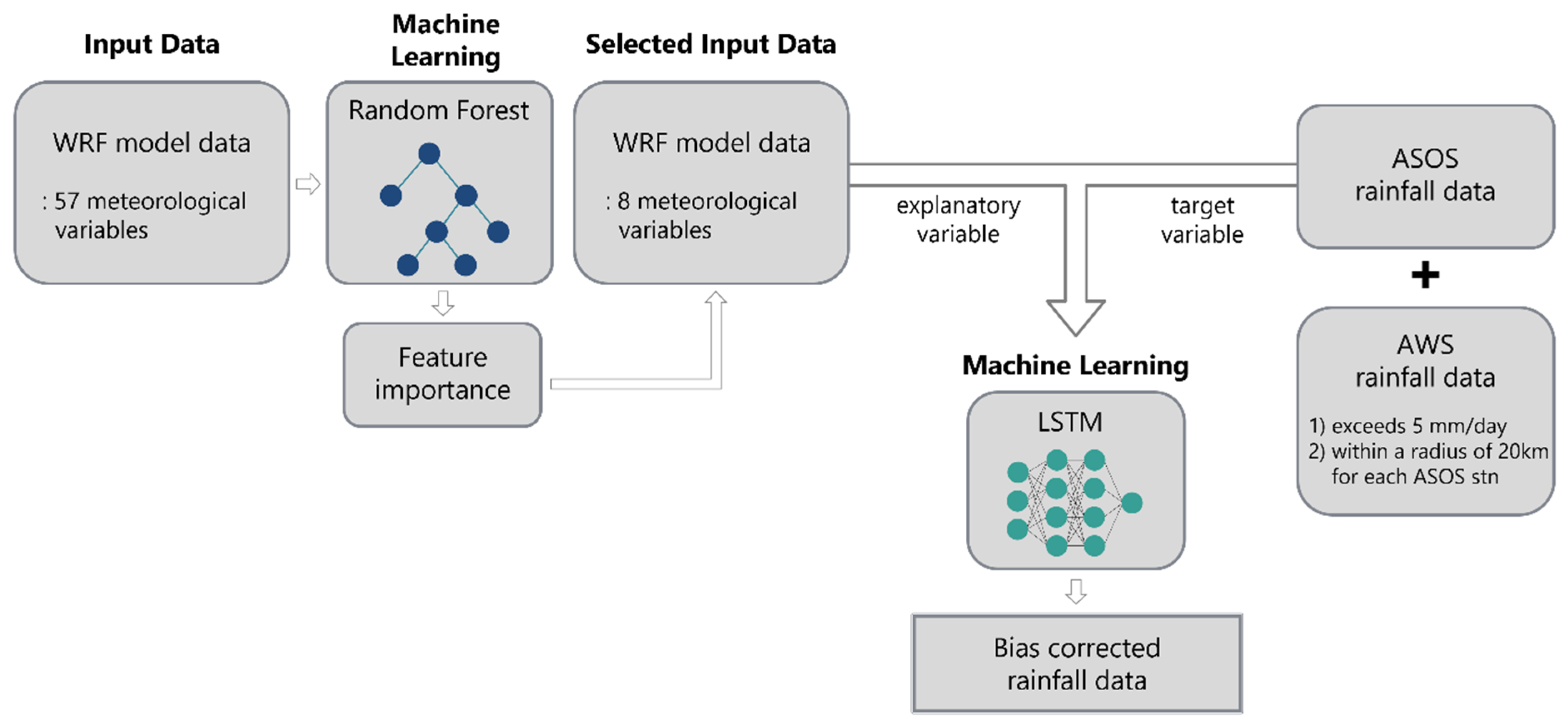
3.1. Bias Correction Method Based on Machine Learning

3.1.1. Long Short-Term Memory (LSTM)

The LSTM machine learning model is used for multivariate bias correction [58]. The LSTM model, a recurrent neural network model, is designed to solve the long-term dependency problem. The LSTM model determines how much memory will be kept or forgotten and exports it as a cell state. Information from the past can be retained by receiving the cell state in the next hidden layer, preventing the gradient vanishing problem. Therefore, the LSTM model shows substantial advantages for problems with sequential data. [59,60,61]. The structure and algorithm equations of LSTM are as follows (Figure 2):

$$i_t=\sigma \left(W_{xi}{x}_t+W_{hi}{h}_{t-1}+b_i\right)$$

(1)

$$f_t=\sigma \left(W_{xf}{x}_t+W_{hf}{h}_{t-1}+b_f\right)$$

(2)

$${\tilde{c}}_t=tanh\left(W_{x\tilde{c}}{x}_t+W_{h\tilde{c}}{h}_{t-1}+b_{\tilde{c}}\right)$$

(3)

$$c_t=f_t\ast c_{t-1}+i_t\ast {\tilde{c}}_t$$

(4)

$$o_t=\sigma (W_{xo}{x}_t+W_{ho}{h}_{t-1}+b_o$$

(5)

$$h_t=o_t\ast tanh\left(c_t\right)$$

(6)

where $i_t$ denotes input gate at a time ($t$), $f_t$ denotes the forget gate, $c_t$ denotes cell state, and $o_t$ denotes the output gate. $x_t$ denotes an input vector and $h_t$ denotes a hidden vector. $W_{xi}, W_{xf}, W_{x\tilde{c}}, W_{xo}$ and $W_{hi},W_{hf},W_{h\tilde{c}}, W_{ho}$ denote the weights of the input vector and hidden vector, respectively, for each gate (i.e., the input gate, forget gate, cell state, and output gate, respectively). $b_i, b_f, b_{\tilde{c}}, b_o$ denote the bias term for each gate. σ is the sigmoid function and $tanh$ is the hyperbolic tangent function.

3.1.2. Process of Bias Correction Using the LSTM Model

The LSTM model can use multiple variables as input features because of its insensitivity to multicollinearity [31,62]. However, using too many or irrelevant input features for the target variable may lead to overfitting [63,64,65]. Therefore, the atmospheric input variables were selected using the Random Forest (RF) machine learning model to train LSTM efficiently. The LSTM model using the input variables filtered for features with low feature importance provides improved results [66,67]. The RF regression model is a bagging tree-based model in which several decision trees are produced with bootstrapping sample datasets and their results are averaged ([68]; Figure 3). The decision tree is a method of partitioning data based on the splitting rule of features until the final partitioning criteria are satisfied [69,70]. The feature importance results can be obtained through RF modeling. The degree of feature importance increases if a specific variable greatly influences data partitioning. In this study, 57 daily atmospheric variables (mean/maximum/minimum temperatures, precipitation, relative humidity, geopotential height, equivalent potential temperature, zonal/meridional/vertical wind variables at the surface, and vertical pressure levels) derived from the WRF model in the 2005–2020 MJJAS were used as input features after normalization, and the normalized ASOS daily rainfall data were used as the target variables of the RF model. RF modeling was performed for each ASOS station by applying leave-one-year-out cross-validation. The leave-one-year-out cross-validation for RF model in this study took one-year data (153 days) from 16 years of data to be used as the test set (~6%) and the remaining 15 years of data to be used as the training set (~94%). Therefore, the total dataset could be generated with 16 training runs for each 66 ASOS stations, and 1056 feature-importance results were produced in this process. Permutation feature importance was also calculated, and similar results were obtained. Considering the feature importance and permutation feature importance results, the eight atmospheric variables that were most frequently ranked in the top five of each feature importance result were selected as input variables for the LSTM model. The selected variables were precipitation, meridional wind at 700 hPa and 850 hPa, equivalent potential temperature at 700 hPa and 500 hPa, relative humidity at 700 hPa and 500 hPa, and zonal wind at 500 hPa. Therefore, the LSTM model was used to perform a bias correction using the eight daily atmospheric variables of the WRF regional climate model interpolated to the ASOS station as explanatory variables and the daily precipitation data of the ASOS station as the target variable.

The optimal hyperparameters of the LSTM model used in this study were configured through a sensitivity test. The LSTM model comprises two LSTM hidden layers and one fully connected layer. The first and second layers using the LSTM layer use 256 and 128 nodes, respectively, and the third fully connected layer with one node is the output layer for correct precipitation. The hyperbolic tangent (tanh) is used as an activation function for the LSTM layers, and the input shape of the LSTM model comprises three timesteps with eight features. Adaptive Moment Estimation (Adam) is used as the optimizer and mean squared error (MSE) is used as the loss function. The batch size is 32 and the epoch is 100 with early stopping. Bias correction using the LSTM model was conducted for each ASOS station with the application of leave-one-year-out cross-validation that considered one-year data (153 days) from 16 years of data as the test set (~6%), another set of one-year data as the validation set (~6%), and the remaining 14 years of data as the training set (~88%) (Figure 4). However, the amount of summertime daily data for 14 years was insufficient for training. Therefore, data showing more than 5 mm/day daily rainfall from the ASOS or AWS stations within a radius of 20 km for the target ASOS station were added to the training data (Figure 5). The 20 km spatial scale was set at which similar precipitation patterns occurred because it was assumed that the spatial scale of precipitation occurring on a daily time scale was approximately 20 km [71]. The WRF explanatory variable data were also interpolated according to the date and location of the additional training data. The bias-corrected result using LSTM was denoted as WRF_LSTM.

3.2. Bias Correction Method Based on Empirical Quantile Mapping

Empirical quantile mapping is a bias correction method that works by fitting the cumulative distribution function (CDF) of the model to that of the observations [8]. In this study, the empirical quantile mapping was performed for each month following previous research [72].

$$P_{WRF, m.d}^{BC}=ECD{F}_{OBS,m}^{-1}\left(ECD{F}_{WRF,m}\left(P_{WRF,m,d}\right)\right)$$

(7)

$P_{WRF,m,d}$ and $P_{WRF, m.d}^{BC}$ denote the WRF_RAW data before and after bias correction (BC) for a specific month ($m$) and date ($d$). $ECD{F}_{WRF,m}$ denotes the CDF of the WRF_RAW for a specific month in the entire period. $ECD{F}_{OBS,m}^{-1}$ denotes the inverse function of the observation CDF for a specific month in the entire period. Leave-one-year-out cross-validation was applied to conduct univariate bias correction for MJJAS daily precipitation using empirical quantile mapping for each ASOS station. That is, a specific one-year (153 days) dataset was denoted as the test dataset, and $ECD{F}_{OBS,m}^{-1}$ and $ECD{F}_{WRF,m}$ were obtained from the observation and WRF data, respectively, for the remaining 15 years except for the year of the test dataset. The test dataset ($P_{WRF,m,d}$) was then corrected, and the process was repeated 16 times to obtain the final bias-corrected data for the entire period. The bias-corrected result using empirical quantile mapping was denoted as the WRF_QM.

3.3. Statistical Assessment Methods

The bias, pattern correlation coefficient (PCC), and normalized standard deviation were calculated to evaluate the model performance quantitatively for the simulated precipitation.

$$Bias=\frac{1}{N}{\displaystyle \sum }_{i=1}^n\left(b_i-o_i\right)$$

(8)

$$PCC=\frac{ {{\displaystyle \sum }}_{i=1}^n\left(b_i-\overline{b}\right)\left(o_i-\overline{o}\right)}{\sqrt{{{\displaystyle \sum }}_{i=1}^n{\left(b_i-\overline{b}\right)}^2} \sqrt{{{\displaystyle \sum }}_{i=1}^n{\left(o_i-\overline{o}\right)}^2}}$$

(9)

$$Normalized standard deviation=\frac{{\sigma }_{BC}}{{\sigma }_{OBS}}$$

(10)

$${\sigma }_x=\sqrt{\frac{1}{n-1}{\displaystyle \sum }_{i=1}^n{\left(x_i-\overline{x}\right)}^2}$$

(11)

$b_i$ and $o_i$ denote the precipitation derived from the model and observations, respectively. ${\sigma }_{OBS}$ and ${\sigma }_{BC}$ denote the spatial standard deviation (σ) of precipitation derived from the WRF_RAW and bias-corrected data, respectively, and n denotes the number of data points.

Additionally, the Root Mean Squared Error (RMSE) and Root Mean Squared Error Skill Score (RMSE-SS) were calculated. The RMSE measures the deviation between an observed value and a bias-corrected value, indicating the accuracy of the bias-corrected data [73]. The RMSE-SS is a normalized measure of the RMSE that presents the capabilities of a bias correction model compared to those of the WRF_RAW [34]. The definition of the calculation formula is as follows:

$$RMSE=\sqrt{{\displaystyle \sum }_{i=1}^n\frac{{\left(b_i-o_i\right)}^2}{n}}$$

(12)

$$RMSE\text{-}SS=1-\frac{RMS{E}_{BC}}{RMS{E}_{RAW}}$$

(13)

$RMS{E}_{RAW}$ and $RMS{E}_{BC}$ denote the RMSEs of precipitation derived from the WRF_RAW and bias-corrected data, respectively. If the RMSE-SS is positive, the bias-corrected precipitation results perform better than the WRF_RAW.

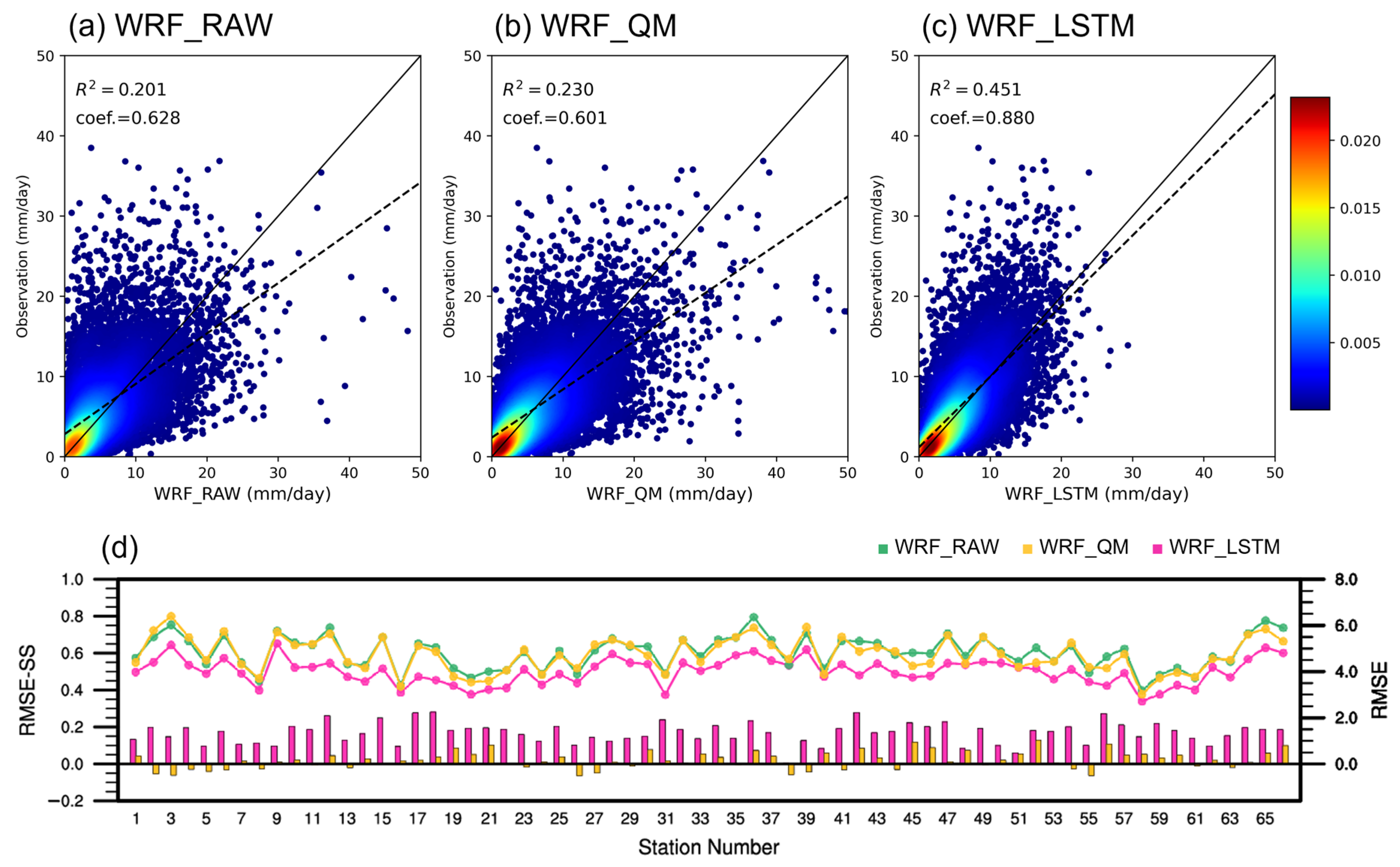
4. Results and Discussion

Figure 6 shows the spatial distribution of summertime (MJJAS) mean rainfall in 2005–2020 and its bias from model data. For ASOS observations, relatively higher precipitation is distributed over the southern coastal and northern regions of South Korea (Figure 6a). The WRF_RAW, the uncorrected WRF model precipitation, shows a dry bias over the entire area of South Korea, except in some stations located near the Taebaek mountains located along the east coast of the Korean Peninsula. In particular, the WRF_RAW underestimates the rainfall in the southern coastal area where high precipitation appears in the observations. The WRF_QM and WRF_LSTM results, in which bias correction has been performed on WRF_RAW data using different methods, show an improved MJJAS rainfall simulation when compared to the WRF_RAW (Figure 6c,d,f,g). A bias magnitude of less than 0.5 mm/day appears at most stations in the WRF_QM. The WRF_QM shows quantitatively good performance for each month and the summertime mean period, representing a spatial correlation coefficient close to 1.0 and a bias and RMSE of less than 0.3 (

Table 1. Statistical assessment of models for each month and MJJAS mean rainfall.

Period	Statistics	WRF_RAW	WRF_QM	WRF_LSTM
MJJAS	Pattern Correlation	0.49	1.00	0.83
	Bias	−0.81	0.16	−0.50
	RMSE	1.10	0.17	0.69
	Normalized Standard deviation	0.85	1.01	1.06
May	Pattern Correlation	0.89	1.00	0.93
	Bias	0.24	0.07	0.16
	RMSE	0.50	0.08	0.39
	Normalized Standard deviation	1.00	1.00	1.00
June	Pattern Correlation	0.81	0.99	0.89
	Bias	0.08	0.17	0.27
	RMSE	0.56	0.22	0.62
	Normalized Standard deviation	1.02	1.03	1.30
July	Pattern Correlation	0.50	1.00	0.88
	Bias	−1.57	0.18	−1.25
	RMSE	2.47	0.21	1.60
	Normalized Standard deviation	0.80	1.00	0.86
August	Pattern Correlation	0.56	1.00	0.66
	Bias	−2.22	0.21	−1.39
	RMSE	2.56	0.24	1.88
	Normalized Standard deviation	1.06	1.00	1.27
September	Pattern Correlation	0.63	0.99	0.76
	Bias	−0.51	0.16	−0.24
	RMSE	1.03	0.20	0.71
	Normalized Standard deviation	1.04	1.04	0.78

). In the case of the WRF_LSTM, the magnitude of the bias is reduced at most stations compared to the WRF_RAW, even though dry bias appears (Figure 6g). The bias correction using the LSTM model was well performed for the summertime period, showing that the magnitudes of the RMSE and bias were lower and the spatial correlation coefficient was higher than that of the WRF_RAW (Table 1). For the monthly statistical verification of the WRF_LSTM rainfall results, the spatial correlation coefficient increased for all months, and the bias and RMSE decreased in all months except for June when compared to the WRF_RAW. The magnitude of the bias decreased by 0.83 mm/day in August, when strong rainfall occurs frequently, indicating a reasonable improvement of the WRF_LSTM.

Figure 7 shows the monthly and interannual variation of MJJAS precipitation. Overall, the model results show reasonable performance. In particular, the WRF_QM simulates the variation closer to the observation than the other model results in the monthly variation (Figure 7a). The average rainfall of each month is similar to the observation because the empirical quantile mapping method fits the CDF of WRF_RAW precipitation to that of the observation for each corresponding month. For the same reason, low bias is also shown in the average of the summertime period (Figure 6f). In the case of the WRF_LSTM for the 2005–2020 mean monthly variation, the results simulated by the WRF_RAW, similar to those of the observation, are maintained without significant correction for the precipitation in May and June. For the period from July to September, which the WRF_RAW underestimates, the WRF_LSTM precipitation is closer to the observation than the WRF_RAW precipitation, and its variation also follows the observation. The advantage of machine learning is that it learns the interrelationship between the climate factors simulated by using the NWP model and performs an accurate bias correction only for the parts that need bias correction, rather than correcting all data uniformly. The WRF_QM shows a similar monthly variation to the observation, but the interannual variation calculated by averaging summertime precipitation every year shows different results (Figure 7b). The WRF_QM shows no improvement after 2008 compared to the WRF_RAW in terms of the variation features. This suggests that quantile mapping has difficulty in correcting sequential features. On the other hand, the WRF_LSTM simulates precipitation close to the observation and represents the overall observed interannual variation pattern well when compared to the WRF_RAW. The WRF_LSTM follows the observed pattern of precipitation increasing from 2008, peaking in 2011, and then decreasing gradually, showing improvement through machine learning-facilitated bias correction. Although the considered period is short, the temporal correlation coefficients of the WRF_RAW, WRF_QM, and WRF_LSTM with the observation are 0.80, 0.78, and 0.86, respectively, indicating the remarkable performance of the WRF_LSTM from the interannual variation perspective.

Figure 8 presents the precipitation results averaged for each day of the year (i.e., calendar day; DOY hereafter). Figure 8a–c show density scatter plots comparing the model-simulated DOY mean precipitation (x-axis) with the ASOS observation (y-axis). The overall distribution of the WRF_QM scatter plot is similar to that of the WRF_RAW (Figure 8a,b). The density above the y = x line is higher than the WRF_RAW in the range of 0–5 mm/day, and the coefficient of determination is 0.230, showing an improvement for the WRF_QM compared to the WRF_RAW. The WRF_LSTM shows much better results than the WRF_RAW and WRF_QM (Figure 8a–c). The coefficient of determination (0.451) and the density above the y = x line in the 0–10 mm/day range are greater for the WRF_LSTM than for the WRF_RAW and WRF_QM. The scatter of the WRF_LSTM is distributed closer to the y = x line than the WRF_RAW and WRF_QM, indicating superior performance. Figure 8d shows the RMSE and RMSE skill scores (RMSE-SS) for each ASOS station. For the RMSE results, the WRF_LSTM shows much lower RMSEs than the WRF_RAW and WRF_QM at all ASOS stations (Figure 8d). In addition, a positive RMSE-SS appears for all ASOS stations in the WRF_LSTM because MSE is used as a loss function in the machine learning process. The WRF_QM exhibits negative RMSE-SS for some stations, and its positive RMSE-SS is smaller than the RMSE-SS of the WRF_LSTM. The WRF_LSTM performs better than the WRF_RAW and WRF_QM for the DOY mean precipitation when considering statistical assessment (e.g., using coefficients of determination and RMSEs). Nevertheless, the WRF_LSTM fails to capture observed DOY mean extreme precipitation greater than 20 mm/day, as shown in the scatter plot (Figure 8c), because there are few cases of extreme precipitation in the training data and the artificial neural network model faces difficulty in solving the extrapolation problem [29,31,74].

In this regard, Figure 9 shows the occurrence frequency for the given model bias and observed daily precipitation to examine the bias according to the observed rainfall amount. The occurrence frequency is shown for the WRF_RAW (Figure 9a). Figure 9b,c illustrates the results obtained by subtracting the occurrence frequency of the WRF_RAW (i.e., Figure 9a) from the bias-corrected data to analyze the changes through a bias correction. The −2-to-2 mm/day bias range (green box), which is considered to simulate the observed precipitation accurately, is enlarged and displayed below the graph. Therefore, a positive value in the green box in Figure 9b,c indicates an improvement with the bias correction.

For the WRF_RAW, a higher frequency of occurrence appears for lighter precipitation (Figure 9a). The frequency of underestimation cases is higher than that of overestimation cases for the total rainfall, particularly for observed rainfall exceeding 100 mm/day. For the occurrence frequency changes in the WRF_QM compared to the WRF_RAW, no distinct pattern appears according to the observed rainfall amount (Figure 9b). The WRF_QM corrects the cases where the WRF_RAW extremely underestimates the less-than-50 mm/day observed rainfall, as negative values appear in these cases. The frequency increases compared to the WRF_RAW for the given 0–30 mm/day wet bias range and 0–5 mm/day observed rainfall. In the green box of the WRF_QM results, positive values appear overall, suggesting that the frequency of well-simulated cases increases in general compared to what occurs in the WRF_RAW. Relatively large positive values are seen for the 3–20 mm/day observed rainfall range, even though negative values appear for below 3 mm/day observed rainfall. In the case of the WRF_LSTM, the overall frequency of the underestimation cases decreases compared to the WRF_RAW (Figure 9c). In particular, the WRF_LSTM shows a larger decrease than the WRF_QM for the cases where the WRF_RAW extremely underestimates the less-than-50 mm/day observed rainfall, suggesting that the WRF_LSTM performs better than the WRF_QM. The WRF_LSTM also shows better performance with a decrease in frequency for the wet bias range exceeding 50 mm/day, while the frequency increases in the WRF_QM. On the other hand, the positive frequency change appears in the WRF_LSTM for cases where observed rainfall exceeding 50 mm/day is underestimated. This suggests some limitations of the WRF_LSTM to capture extreme precipitation, which aligns with Figure 8c. For the −2-to-2 mm/day bias range in the WRF_LSTM (see the green box of Figure 9c), the negative values appear for below 10 mm/day observed rainfall, corresponding to an increase in the frequency of overestimated cases compared to the WRF_RAW for the observed weak rainfall. For 10–50 mm/day observed precipitation (the range of the cyan line in Figure 9c), however, a significant positive value appears that is larger than the WRF_QM. This indicates the better correction performance of the WRF_LSTM than the WRF_QM for light-to-moderate rainfall. The 10–50 mm/day observed rainfall falls within the 50–90th percentile and accounts for 38.8% occurrence frequency in South Korea. In addition, it accounts for 34–56% of the summertime accumulated rainfall and has a prominent interannual variation over South Korea. These results suggest that the improvement of simulating 10–50 mm/day precipitation in the WRF_LSTM contributes sufficiently to the improvement of the climatological mean and interannual variation simulation of summertime rainfall.

Figure 10 shows the distribution of the daily precipitation RMSE according to the rainfall amount using a boxplot. Here, the RMSE is calculated for daily rainfall events corresponding to specific rainfall ranges for each ASOS station and month. For all rainfall ranges (exceeding 1 mm/day), relatively larger RMSEs appear in July and August (Figure 10a). The bias-corrected results generally show similar or improved results compared to the WRF_RAW. For the WRF_QM, the medians are similar to those of the WRF_RAW, except for September, where a higher median appears. The WRF_QM has lower maximum RMSEs than the WRF_RAW in May and June, despite exhibiting higher maximum values than the other models in July through September. In the case of the WRF_LSTM, the overall RMSE distribution is lower than the other models, indicating good performance in correcting bias. These results are also observed in weak precipitation (1–10 mm/day; Figure 10b) and light-to-moderate precipitation (10–50 mm/day; Figure 10c), particularly in the latter rainfall range. For weak precipitation, although the median and the box of the WRF_LSTM are still lower than WRF_RAW, they appear within a similar range to the other models. For light-to-moderate precipitation, the RMSE distribution of the WRF_LSTM is much lower than that of the other models, showing a significant difference. This result aligns with the abovementioned results that show that the WRF_LSTM has strength in correcting light-to-moderate precipitation (Figure 9). For extreme precipitation (>50 mm/day; Figure 10d), the WRF_QM shows improved performance in August, while it presents similar RMSE distributions to the WRF_RAW in June and September. Although the maximum for the WRF_QM is higher, its median is lower than the WRF_RAW in July. In the case of the WRF_LSTM, the medians appear lower than those of the WRF_RAW from June through September. This indicates the degree of the potential for the WRF_LSTM to perform an accurate bias correction for extreme precipitation. Although the WRF_LSTM shows a higher maximum RMSE than the WRF_RAW in July, it performs better in other months (June, August, and September) by presenting a lower median and maximum RMSE than the WRF_RAW.

5. Summary and Conclusions

This study compared bias correction methods using empirical quantile mapping and machine learning models for the summertime daily rainfall in South Korea, which was simulated by the high-resolution WRF model. For machine learning bias correction, the LSTM model was used, with eight meteorological variables derived from the WRF model being used as the input variables. The empirical quantile mapping was performed for every month. The results were compared with the machine learning bias correction results in terms of daily precipitation.

The WRF_QM and WRF_LSTM showed better performance for the MJJAS mean rainfall spatial distribution than the WRF_RAW. The WRF_QM presented a smaller bias magnitude than the WRF_RAW for most ASOS stations and a higher spatial correlation coefficient (close to 1.0). Since the empirical quantile mapping method fit the CDF of the WRF_RAW precipitation to that of the observation for each corresponding month, the mean rainfall amount of the WRF_QM for each month and the MJJAS period showed good agreement with the observation. In the case of the WRF_LSTM, the bias magnitude of the MJJAS mean rainfall was reduced in most ASOS stations compared to the WRF_RAW. On the other hand, the WRF_LSTM represented a similar interannual variation of rainfall to the observations compared to the WRF_RAW, while the WRF_QM showed no improvement. In addition, the coefficient of determination was the highest in the order of the WRF_LSTM, WRF_QM, and WRF_RAW for the mean rainfall amount for each calendar day.

The occurrence frequencies for the given observed daily rainfall and model bias were analyzed. The frequency of well-simulated cases increased overall in the WRF_QM compared to the WRF_RAW. The WRF_LSTM corrected the bias more efficiently than the WRF_QM for the cases where the WRF_RAW extremely underestimated an observed rainfall of less than 50 mm/day. On the other hand, the WRF_LSTM showed a certain limitation in capturing observed extreme rainfall of over 50 mm/day. For the 10–50 mm/day observed precipitation, the WRF_LSTM outperformed the WRF_RAW and WRF_QM, showing the highest number of well-simulated cases among the three. The WRF_LSTM also had a much lower RMSE than the other models in the 10–50 mm/day range, indicating good performance in correcting bias. This suggests that the bias correction method of WRF_LSTM is performed commendably for light-to-moderate rainfall.

The results of this study suggest that the bias correction method using the LSTM model can be used sufficiently for precipitation bias correction. The aim was to train an LSTM model bias correction method that could cover the entire range of precipitation, even though the results showed different performances depending on the rainfall amounts. Several reasons could have contributed to these discrepancies. First, machine learning models often show weakness when dealing with imbalanced datasets [38,74]. As mentioned in Figure 8, the number of daily extreme rainfall cases in the data was lower than that of the other precipitation levels because of the relatively low occurrence frequency of extreme rainfall events. Second, the LSTM model, being a sequence-based model, may not have captured all relevant spatial information [75]. Extreme rainfall events often involve localized and highly spatially heterogeneous patterns, which may be critical to accurate reproduction. Hence, the capability to depict extreme precipitation will increase as the analysis period is extended and more data on extreme rainfall accumulates. Furthermore, the LSTM model might need to be combined with spatially aware models or retrained with additional spatial features to improve its performance in these cases. Based on the results of this study, which utilized dynamically downscaled reanalysis data, further research will require bias corrections to downscale the forecast precipitation data.

References

1. Teng, J.; Potter, N.J.; Chiew, F.H.S.; Zhang, L.; Wang, B.; Vaze, J.; Evans, J.P. How does bias correction of regional climate model precipitation affect modelled runoff? Hydrol. Earth Syst. Sci. 2015, 19, 711–728. [Google Scholar] [CrossRef] [Green Version]
2. Wood, A.W.; Leung, L.R.; Sridhar, V.; Lettenmaier, D.P. Hydrologic Implications of Dynamical and Statistical Approaches to Downscaling Climate Model Outputs. Clim. Change 2004, 62, 189–216. [Google Scholar] [CrossRef]
3. Velasquez, P.; Messmer, M.; Raible, C.C. A new bias-correction method for precipitation over complex terrain suitable for different climate states: A case study using WRF (version 3.8.1). Geosci. Model Dev. 2020, 13, 5007–5027. [Google Scholar] [CrossRef]
4. Thrasher, B.; Maurer, E.P.; McKellar, C.; Duffy, P.B. Technical Note: Bias correcting climate model simulated daily temperature extremes with quantile mapping. Hydrol. Earth Syst. Sci. 2012, 16, 3309–3314. [Google Scholar] [CrossRef] [Green Version]
5. Teutschbein, C.; Seibert, J. Bias correction of regional climate model simulations for hydrological climate-change impact studies: Review and evaluation of different methods. J. Hydrol. 2012, 456–457, 12–29. [Google Scholar] [CrossRef]
6. Kim, G.; Cha, D.-H.; Lee, G.; Park, C.; Jin, C.-S.; Lee, D.-K.; Suh, M.-S.; Ahn, J.-B.; Min, S.-K.; Kim, J. Projection of future precipitation change over South Korea by regional climate models and bias correction methods. Theor. Appl. Climatol. 2020, 141, 1415–1429. [Google Scholar] [CrossRef]
7. Jeong, H.-G.; Ahn, J.-B.; Lee, J.; Shim, K.-M.; Jung, M.-P. Improvement of daily precipitation estimations using PRISM with inverse-distance weighting. Theor. Appl. Climatol. 2020, 139, 923–934. [Google Scholar] [CrossRef] [Green Version]
8. Gudmundsson, L.; Bremnes, J.B.; Haugen, J.E.; Engen-Skaugen, T. Technical Note: Downscaling RCM precipitation to the station scale using statistical transformations – a comparison of methods. Hydrol. Earth Syst. Sci. 2012, 16, 3383–3390. [Google Scholar] [CrossRef] [Green Version]
9. Cannon, A.J.; Sobie, S.R.; Murdock, T.Q. Bias Correction of GCM Precipitation by Quantile Mapping: How Well Do Methods Preserve Changes in Quantiles and Extremes? J. Clim. 2015, 28, 6938–6959. [Google Scholar] [CrossRef]
10. Song, C.-Y.; Kim, S.-H.; Ahn, J.-B. Improvement in Seasonal Prediction of Precipitation and Drought over the United States Based on Regional Climate Model Using Empirical Quantile Mapping. Atmosphere 2021, 31, 637–656, (In Korean with English Abstract). [Google Scholar]
11. Lafon, T.; Dadson, S.; Buys, G.; Prudhomme, C. Bias correction of daily precipitation simulated by a regional climate model: A comparison of methods. Int. J. Climatol. 2013, 33, 1367–1381. [Google Scholar] [CrossRef] [Green Version]
12. Li, H.; Sheffield, J.; Wood, E.F. Bias correction of monthly precipitation and temperature fields from Intergovernmental Panel on Climate Change AR4 models using equidistant quantile matching. J. Geophys. Res. Atmos. 2010, 115, D10101. [Google Scholar] [CrossRef]
13. Luo, X.; Fan, X.; Li, Y.; Ji, X. Bias correction of a gauge-based gridded product to improve extreme precipitation analysis in the Yarlung Tsangpo–Brahmaputra River basin. Nat. Hazards Earth Syst. Sci. 2020, 20, 2243–2254. [Google Scholar] [CrossRef]
14. Rajczak, J.; Kotlarski, S.; Schär, C. Does Quantile Mapping of Simulated Precipitation Correct for Biases in Transition Probabilities and Spell Lengths? J. Clim. 2016, 29, 1605–1615. [Google Scholar] [CrossRef]
15. Cannon, A.J. Multivariate quantile mapping bias correction: An N-dimensional probability density function transform for climate model simulations of multiple variables. Clim. Dyn. 2018, 50, 31–49. [Google Scholar] [CrossRef] [Green Version]
16. Wang, F.; Tian, D. On deep learning-based bias correction and downscaling of multiple climate models simulations. Clim. Dyn. 2022, 59, 3451–3468. [Google Scholar] [CrossRef]
17. Meyer, J.; Kohn, I.; Stahl, K.; Hakala, K.; Seibert, J.; Cannon, A.J. Effects of univariate and multivariate bias correction on hydrological impact projections in alpine catchments. Hydrol. Earth Syst. Sci. 2019, 23, 1339–1354. [Google Scholar] [CrossRef] [Green Version]
18. Mehrotra, R.; Sharma, A. Correcting for systematic biases in multiple raw GCM variables across a range of timescales. J. Hydrol. 2015, 520, 214–223. [Google Scholar] [CrossRef]
19. Li, C.; Sinha, E.; Horton, D.E.; Diffenbaugh, N.S.; Michalak, A.M. Joint bias correction of temperature and precipitation in climate model simulations. J. Geophys. Res. Atmos. 2014, 119, 13,153–113,162. [Google Scholar] [CrossRef]
20. Hong, J.; Kim, T.Y.; Park, J.-S. Multivariate Bias Correction for Climate Simulation Data, with Application to Precipitation Extremes in Korea. Quant. Bio-Sci. 2019, 38, 121–130. [Google Scholar] [CrossRef]
21. Sun, Q.; Miao, C.; Qiao, Y.; Duan, Q. The nonstationary impact of local temperature changes and ENSO on extreme precipitation at the global scale. Clim. Dyn. 2017, 49, 4281–4292. [Google Scholar] [CrossRef]
22. Choi, Y.-W.; Ahn, J.-B. Possible mechanisms for the coupling between late spring sea surface temperature anomalies over tropical Atlantic and East Asian summer monsoon. Clim. Dyn. 2019, 53, 6995–7009. [Google Scholar] [CrossRef] [Green Version]
23. Ha, K.-J.; Heo, K.-Y.; Lee, S.-S.; Yun, K.-S.; Jhun, J.-G. Variability in the East Asian Monsoon: A review. Meteorol. Appl. 2012, 19, 200–215. [Google Scholar] [CrossRef]
24. Gibson, P.B.; Chapman, W.E.; Altinok, A.; Delle Monache, L.; DeFlorio, M.J.; Waliser, D.E. Training machine learning models on climate model output yields skillful interpretable seasonal precipitation forecasts. Commun. Earth Environ. 2021, 2, 159. [Google Scholar] [CrossRef]
25. Kim, H.; Ham, Y.G.; Joo, Y.S.; Son, S.W. Deep learning for bias correction of MJO prediction. Nat. Commun. 2021, 12, 3087. [Google Scholar] [CrossRef]
26. Estébanez-Camarena, M.; Curzi, F.; Taormina, R.; van de Giesen, N.; ten Veldhuis, M.-C. The Role of Water Vapor Observations in Satellite Rainfall Detection Highlighted by a Deep Learning Approach. Atmosphere 2023, 14, 974. [Google Scholar] [CrossRef]
27. Rolnick, D.; Donti, P.L.; Kaack, L.H.; Kochanski, K.; Lacoste, A.; Sankaran, K.; Ross, A.S.; Milojevic-Dupont, N.; Jaques, N.; Waldman-Brown, A.; et al. Tackling Climate Change with Machine Learning. ACM Comput. Surv. 2022, 55, 1–96. [Google Scholar] [CrossRef]
28. Jiang, H.; Hu, H.; Zhong, R.; Xu, J.; Xu, J.; Huang, J.; Wang, S.; Ying, Y.; Lin, T. A deep learning approach to conflating heterogeneous geospatial data for corn yield estimation: A case study of the US Corn Belt at the county level. Glob. Change Biol. 2020, 26, 1754–1766. [Google Scholar] [CrossRef]
29. Li, X.; Li, Z.; Huang, W.; Zhou, P. Performance of statistical and machine learning ensembles for daily temperature downscaling. Theor. Appl. Climatol. 2020, 140, 571–588. [Google Scholar] [CrossRef]
30. Tao, Y.; Hsu, K.; Ihler, A.; Gao, X.; Sorooshian, S. A Two-Stage Deep Neural Network Framework for Precipitation Estimation from Bispectral Satellite Information. J. Hydrometeorol. 2018, 19, 393–408. [Google Scholar] [CrossRef]
31. Cho, D.; Yoo, C.; Im, J.; Cha, D.H. Comparative Assessment of Various Machine Learning-Based Bias Correction Methods for Numerical Weather Prediction Model Forecasts of Extreme Air Temperatures in Urban Areas. Earth Space Sci. 2020, 7, e2019EA000740. [Google Scholar] [CrossRef] [Green Version]
32. Song, Y.H.; Chung, E.-S.; Shiru, M.S. Uncertainty Analysis of Monthly Precipitation in GCMs Using Multiple Bias Correction Methods under Different RCPs. Sustainability 2020, 12, 7508. [Google Scholar] [CrossRef]
33. Tan, J.; Chen, S.; Lee, C.Y.; Dong, G.; Hu, W.; Wang, J. Projected changes of typhoon intensity in a regional climate model: Development of a machine learning bias correction scheme. Int. J. Climatol. 2021, 41, 2749–2764. [Google Scholar] [CrossRef]
34. Tao, Y.; Yang, T.; Faridzad, M.; Jiang, L.; He, X.; Zhang, X. Non-stationary bias correction of monthly CMIP5 temperature projections over China using a residual-based bagging tree model. Int. J. Climatol. 2018, 38, 467–482. [Google Scholar] [CrossRef]
35. Zhang, C.-J.; Zeng, J.; Wang, H.-Y.; Ma, L.-M.; Chu, H. Correction model for rainfall forecasts using the LSTM with multiple meteorological factors. Meteorol. Appl. 2020, 27, e1852. [Google Scholar] [CrossRef] [Green Version]
36. Fouotsa Manfouo, N.C.; Potgieter, L.; Watson, A.; Nel, J.H. A Comparison of the Statistical Downscaling and Long-Short-Term-Memory Artificial Neural Network Models for Long-Term Temperature and Precipitations Forecasting. Atmosphere 2023, 14, 708. [Google Scholar] [CrossRef]
37. Lee, S.; Kim, J.; Lee, G.; Hong, J.; Bae, J.H.; Lim, K.J. Prediction of Aquatic Ecosystem Health Indices through Machine Learning Models Using the WGAN-Based Data Augmentation Method. Sustainability 2021, 13, 10435. [Google Scholar] [CrossRef]
38. He, H.; Garcia, E.A. Learning from Imbalanced Data. IEEE Trans. Knowl. Data Eng. 2009, 21, 1263–1284. [Google Scholar] [CrossRef]
39. Hess, P.; Boers, N. Deep Learning for Improving Numerical Weather Prediction of Heavy Rainfall. J. Adv. Model. Earth Syst. 2022, 14, e2021MS002765. [Google Scholar] [CrossRef]
40. Jung, H.-S.; Lim, G.-H.; Oh, J.-H. Interpretation of the Transient Variations in the Time Series of Precipitation Amounts in Seoul, Korea. Part I: Diurnal Variation. J. Clim. 2001, 14, 2989–3004. [Google Scholar] [CrossRef]
41. Kim, W.; Jhun, J.-G.; Ha, K.-J.; Kimoto, M. Decadal changes in climatological intraseasonal fluctuation of subseasonal evolution of summer precipitation over the Korean Peninsula in the mid-1990s. Adv. Atmos. Sci. 2011, 28, 591–600. [Google Scholar] [CrossRef]
42. Lee, J.-Y.; Kwon, M.; Yun, K.-S.; Min, S.-K.; Park, I.-H.; Ham, Y.-G.; Jin, E.K.; Kim, J.-H.; Seo, K.-H.; Kim, W.; et al. The long-term variability of Changma in the East Asian summer monsoon system: A review and revisit. Asia-Pac. J. Atmos. Sci. 2017, 53, 257–272. [Google Scholar] [CrossRef]
43. Seo, K.-H.; Son, J.-H.; Lee, J.-Y.; Park, H.-S. Northern East Asian Monsoon Precipitation Revealed by Airmass Variability and Its Prediction. J. Clim. 2015, 28, 6221–6233. [Google Scholar] [CrossRef]
44. Skamarock, C.; Klemp, B.; Dudhia, J.; Gill, O.; Liu, Z.; Berner, J.; Wang, W.; Powers, G.; Duda, G.; Barker, D.; et al. A Description of the Advanced Research WRF Model Version 4; National Center for Atmospheric Research: Boulder, CO, USA, 2019. [Google Scholar]
45. Giorgi, F.; Mearns, L.O. Approaches to the simulation of regional climate change: A review. Rev. Geophys. 1991, 29, 191–216. [Google Scholar] [CrossRef]
46. Benestad, R. Downscaling Climate Information. In Oxford Research Encyclopedia of Climate Science; Oxford University Press: Oxford, UK, 2016. [Google Scholar] [CrossRef]
47. Giorgi, F. Thirty Years of Regional Climate Modeling: Where Are We and Where Are We Going next? J. Geophys. Res. Atmos. 2019, 124, 5696–5723. [Google Scholar] [CrossRef] [Green Version]
48. Hersbach, H.; Bell, B.; Berrisford, P.; Hirahara, S.; Horányi, A.; Muñoz-Sabater, J.; Nicolas, J.; Peubey, C.; Radu, R.; Schepers, D.; et al. The ERA5 global reanalysis. Q. J. R. Meteorol. Soc. 2020, 146, 1999–2049. [Google Scholar] [CrossRef]
49. Harris, L.M.; Durran, D.R. An Idealized Comparison of One-Way and Two-Way Grid Nesting. Mon. Weather Rev. 2010, 138, 2174–2187. [Google Scholar] [CrossRef] [Green Version]
50. Liu, J.; Bray, M.; Han, D. Sensitivity of the Weather Research and Forecasting (WRF) model to downscaling ratios and storm types in rainfall simulation. Hydrol. Process. 2012, 26, 3012–3031. [Google Scholar] [CrossRef]
51. Wang, S.; Yu, E.; Wang, H. A simulation study of a heavy rainfall process over the Yangtze River valley using the two-way nesting approach. Adv. Atmos. Sci. 2012, 29, 731–743. [Google Scholar] [CrossRef]
52. Chen, F.; Dudhia, J. Coupling an Advanced Land Surface–Hydrology Model with the Penn State–NCAR MM5 Modeling System. Part I: Model Implementation and Sensitivity. Mon. Weather Rev. 2001, 129, 569–585. [Google Scholar] [CrossRef]
53. Tao, W.-K.; Simpson, J.; McCumber, M. An Ice-Water Saturation Adjustment. Mon. Weather Rev. 1989, 117, 231–235. [Google Scholar] [CrossRef]
54. Tao, Y.; Cao, J.; Lan, G.; Su, Q. The zonal movement of the Indian–East Asian summer monsoon interface in relation to the land–sea thermal contrast anomaly over East Asia. Clim. Dyn. 2016, 46, 2759–2771. [Google Scholar] [CrossRef]
55. Hong, S.-Y.; Noh, Y.; Dudhia, J. A New Vertical Diffusion Package with an Explicit Treatment of Entrainment Processes. Monthly Weather Review 2006, 134, 2318–2341. [Google Scholar] [CrossRef] [Green Version]
56. Collins, W.D.; Hackney, J.K.; Edwards, D.P. An updated parameterization for infrared emission and absorption by water vapor in the National Center for Atmospheric Research Community Atmosphere Model. J. Geophys. Res. 2002, 107, ACL 17-11-ACL 17-20. [Google Scholar] [CrossRef]
57. Kain, J.S. The Kain–Fritsch Convective Parameterization: An Update. J. Appl. Meteorol. 2004, 43, 170–181. [Google Scholar] [CrossRef]
58. Hochreiter, S.; Schmidhuber, J. Long Short-Term Memory. Neural Comput. 1997, 9, 1735–1780. [Google Scholar] [CrossRef] [PubMed]
59. Yu, Y.; Si, X.; Hu, C.; Zhang, J. A Review of Recurrent Neural Networks: LSTM Cells and Network Architectures. Neural Comput. 2019, 31, 1235–1270. [Google Scholar] [CrossRef]
60. Islam, M.S.; Sharmin Mousumi, S.S.; Abujar, S.; Hossain, S.A. Sequence-to-sequence Bangla Sentence Generation with LSTM Recurrent Neural Networks. Procedia Comput. Sci. 2019, 152, 51–58. [Google Scholar] [CrossRef]
61. Li, W.; Kiaghadi, A.; Dawson, C. High temporal resolution rainfall–runoff modeling using long-short-term-memory (LSTM) networks. Neural Comput. Appl. 2021, 33, 1261–1278. [Google Scholar] [CrossRef]
62. Thorp, K.R.; Drajat, D. Deep machine learning with Sentinel satellite data to map paddy rice production stages across West Java, Indonesia. Remote Sens. Environ. 2021, 265, 112679. [Google Scholar] [CrossRef]
63. Bagherzadeh, F.; Mehrani, M.-J.; Basirifard, M.; Roostaei, J. Comparative study on total nitrogen prediction in wastewater treatment plant and effect of various feature selection methods on machine learning algorithms performance. J. Water Process Eng. 2021, 41, 102033. [Google Scholar] [CrossRef]
64. Ranjan, K.G.; Prusty, B.R.; Jena, D. Review of preprocessing methods for univariate volatile time-series in power system applications. Electr. Power Syst. Res. 2021, 191, 106885. [Google Scholar] [CrossRef]
65. Luengo, J.; García-Gil, D.; Ramírez-Gallego, S.; García, S.; Herrera, F. Big Data Preprocessing; Springer: Cham, Switzerland, 2020. [Google Scholar]
66. Lin, S.; Tian, H. Short-Term Metro Passenger Flow Prediction Based on Random Forest and LSTM. In Proceedings of the 2020 IEEE 4th Information Technology, Networking, Electronic and Automation Control Conference (ITNEC), Chongqing, China, 12–14 June 2020; pp. 2520–2526. [Google Scholar]
67. Jiang, X.; Liu, Y.; Ye, X. Short-Term Prediction of Global Temperature Based on RF Feature Subset Selection and PSO-LSTM model. In Proceedings of the 2021 6th International Symposium on Computer and Information Processing Technology (ISCIPT), Changsha, China, 11–13 June 2021; pp. 67–72. [Google Scholar]
68. Breiman, L. Random Forests. Mach. Learn. 2001, 45, 5–32. [Google Scholar] [CrossRef] [Green Version]
69. Breiman, L.; Friedman, J.; Stone, C.J.; Olshen, R.A. Classification and Regression Trees; Taylor & Francis: Abingdon, UK, 1984. [Google Scholar]
70. Tso, G.K.F.; Yau, K.K.W. Predicting electricity energy consumption: A comparison of regression analysis, decision tree and neural networks. Energy 2007, 32, 1761–1768. [Google Scholar] [CrossRef]
71. Orlanski, I. A Rational Subdivision of Scales for Atmospheric Processes. Bull. Am. Meteorol. Soc. 1975, 56, 527–530. [Google Scholar]
72. Reiter, P.; Gutjahr, O.; Schefczyk, L.; Heinemann, G.; Casper, M. Does applying quantile mapping to subsamples improve the bias correction of daily precipitation? Int. J. Climatol. 2018, 38, 1623–1633. [Google Scholar] [CrossRef]
73. Dai, Y.; Lu, Z.; Zhang, H.; Zhan, T.; Lu, J.; Wang, P. A Correction Method of Environmental Meteorological Model Based on Long-Short-Term Memory Neural Network. Earth Space Sci. 2019, 6, 2214–2226. [Google Scholar] [CrossRef] [Green Version]
74. Marcus, G.F. Deep Learning: A Critical Appraisal. arXiv 2018, arXiv:1801.00631. [Google Scholar]
75. Shi, X.; Chen, Z.; Wang, H.; Yeung, D.-Y.; Wong, W.-K.; Woo, W.-C. Convolutional LSTM Network: A machine learning approach for precipitation nowcasting. In Proceedings of the 28th International Conference on Neural Information Processing Systems—Volume 1, Montreal, QC, Canada, 7–12 December 2015; pp. 802–810. [Google Scholar]
Figure 1. (a) Topography (units: m) of WRF simulation domain and (b) locations of ASOS (green dot) and AWS (small black dot) stations. The number in each green dot denotes the ASOS station number.
Atmosphere 14 01057 g001
Figure 2. Structure of the LSTM model.
Atmosphere 14 01057 g002
Figure 3. Schematic diagram of the Random Forest model.
Atmosphere 14 01057 g003
Figure 4. Schematic of leave-one year-out cross-validation.
Atmosphere 14 01057 g004
Figure 5. Schematic diagram of the bias correction process using the machine learning model.
Atmosphere 14 01057 g005
Figure 6. Spatial distribution of MJJAS mean precipitation (units: mm/day) at ASOS stations derived from (a) observation (ASOS), (b) WRF_RAW, (c) WRF_QM, and (d) WRF_LSTM and model biases for (e) WRF_RAW, (f) WRF_QM, and (g) WRF_LSTM.
Atmosphere 14 01057 g006
Figure 7. (a) Monthly variation of each year and 2005–2020 averaged precipitation (units: mm/day) and (b) interannual variation of the MJJAS mean precipitation (units: mm/day).
Atmosphere 14 01057 g007
Figure 8. Density scatter plot for rainfall derived from ASOS and rainfall derived from (a) WRF_RAW, (b) WRF_QM, and (c) WRF_LSTM and (d) RMSE (line chart) and RMSE-SS (bar chart) for each ASOS station.
Atmosphere 14 01057 g008
Figure 9. (a) Occurrence frequency (units: 0.0001%) of given observed rainfall (x-axis) and WRF_RAW bias (y-axis) for MJJAS and the difference of occurrence frequencies (units: 0.0001%) between WRF_RAW, (b) WRF_QM, and (c) WRF_LSTM results. The bias in the range of −2-to-2 mm/day (green box) is enlarged for each figure.
Atmosphere 14 01057 g009
Figure 10. Boxplot of the RMSE (units: mm/day) according to the observed rainfall amounts for (a) all rainfall events, (b) 1–10 mm/day, (c) 10–50 mm/day, and (d) over 50 mm/day.
Atmosphere 14 01057 g010