
The Local Unscented Transform Kalman Filter for the Weather Research and Forecasting Model

Department of Software, Sangmyung University, Cheonan-si 31066, Republic of Korea
Atmosphere 2023, 14(7), 1143; https://doi.org/10.3390/atmos14071143
Submission received: 5 June 2023
/
Revised: 3 July 2023
/
Accepted: 8 July 2023
/
Published: 13 July 2023
(This article belongs to the Section Climatology)
Abstract
:In this study, the local unscented transform Kalman filter (LUTKF) proposed in the previous study estimates the state of the Weather Research and Forecasting (WRF) model through local analysis. Real observations are assimilated to investigate the analysis performance of the WRF-LUTKF system. The WRF model as a regional numerical weather prediction (NWP) model is widely used to explain the atmospheric state for mesoscale meteorological fields, such as operational forecasting and atmospheric research applications. For the LUTKF based on the sigma-point Kalman filter (SPKF), the state of the nonlinear system is estimated by propagating ensemble members through the unscented transformation (UT) without making any linearization assumptions for nonlinear models. The main objective of this study is to examine the feasibility of mesoscale data assimilations for the LUTKF algorithm using the WRF model and real observations. Similar to the local ensemble transform Kalman filter (LETKF), by suppressing the impact of distant observations on model state variables through localization schemes, the LUTKF can eliminate spurious long-distance correlations in the background covariance, which are induced by the sampling error due to the finite ensemble size; therefore, the LUTKF used in the WRF-LUTKF system can efficiently execute the data assimilation with a small ensemble size. Data assimilation test results demonstrate that the LUTKF can provide reliable analysis performance in estimating the WRF model state with real observations. Experiments with various ensemble size show that the LETKF can provide better estimation results with a larger ensemble size, while the LUTKF can achieve accurate and reliable assimilation results even with a smaller ensemble size.
1. Introduction
The data assimilation is used to capture the observation information in an effective manner and to offer accurate initial conditions when the state of the numerical weather prediction (NWP) model is estimated. Currently, most data assimilation systems can be classified into variational-based and ensemble-based schemes: variational-based methods are divided into the three-dimensional variational (3DVAR) [1,2] and four-dimensional variational (4DVAR) [3,4] data assimilation algorithms; and ensemble-based techniques are organized into the ensemble Kalman filter (EnKF) [5] and its variants, such as the ensemble square root filter (EnSRF) [6] and the local ensemble transform Kalman filter (LETKF) [7].
The ensemble-based schemes provide the following advantages over the variational-based methods: (i) the forecast uncertainty (background error covariance) in ensemble-based schemes is directly obtained by propagating ensemble members; (ii) unlike the 4DVAR, they can be easily implemented without the tangent linear and adjoint models required for the 4DVAR; and (iii) they can be also computationally efficient due to the local analysis and covariance inflation, especially for the LETKF in parallel computer architecture. The ensemble variational (EnVAR) algorithm, which is a hybrid combination for both data assimilation approaches, has been studied to improve the assimilation performance by leveraging the advantages of both methods [8,9,10].
Recently, the sigma-point Kalman filter (SPKF) was introduced to estimate the state of atmospheric and oceanic models in the meteorological fields [11,12,13]. The SPKF and existing ensemble-based Kalman filters (EBKFs), such as the EnKF and its variations, differ in the ensemble sampling and ensemble size determination. For the L-dimensional system, the ensemble sampling of the SPKF is executed by deterministically selecting ensemble members, which are also referred to as sigma points, through the unscented transformation (UT) to enable them to have statistical properties of the system. The deterministically chosen ensemble members are propagated to calculate the mean and covariance of the nonlinear model state using model equations. Different from the existing EBKF methods, the SPKF scheme also makes no linearization assumption for nonlinear prediction and observation models; that is, it can compute statistical moments (mean and covariance) of the nonlinear model state using fully nonlinear prediction and observation operators by reinterpreting the analysis phase of the EBKFs, including the Kalman gain calculation.
However, since the SPKF approach estimates the model state with ensemble members for the L-dimensional system, it can require substantial computational resources for high-dimensional systems. In addition, because the model state vector estimated in the SPKF is augmented by the concatenation of the original model state variables, model noise, and observation noise, its dimensionality is equal to the sum of the original model state, model noise, and observation noise dimensional numbers. Thus, the SPKF can require prohibitively computationally expensive costs when assimilating considerable observations in a nonlinear model with high dimensionality.
Some solutions to the problem have been introduced. One method reduces the ensemble size in order to use only effective ensemble members for the data assimilation; for example, only the ensemble members that have a great impact on the estimate of the L-dimensional model state are used during every data assimilation cycle [14]. Another scheme is to use the principal component analysis (PCA), which can infer the model state with a smaller ensemble size in the principal component space while maintaining the main characteristics in the full ensemble space [15]; that is, this scheme that uses fewer ensemble members than are used in the full ensemble space can provide state estimation results that are as accurate as the original SPKF. The other solution to the problem is to reduce the ensemble size by truncating the error covariance matrix through the singular value decomposition (SVD). As a result, this method can execute the state estimation with lower computational times than those in the original SPKF. However, for the oceanic and atmospheric system with a high dimensionality, the methods described above can still require considerable computational costs when a large number of observations are assimilated to the model state.
The localization approach can be used to solve the problem with the computational difficulty for high-dimensional models. For high-dimensional models, it enables the EBKFs to efficiently execute the local data assimilation with a small number of ensemble members at each model grid point. However, the SPKF algorithm (known as a global filter) carries out the data assimilation using the augmented state vector that consists of model state variables, process noises, and measurement noises for all model grid points in the global domain. For this reason, the SPKF that uses the augmented state vector can struggle to perform the local analysis for high-dimensional models using the localization approach.
Unlike the SPKF scheme, the local unscented transform Kalman filter algorithm proposed in the previous study (LUTKF) [13] is based on the non-augmented state vector; thus, it can perform data assimilation using the state vector that is composed of only the model state variables. This enables the localization scheme to be easily applied to the LUTKF. The localization approach applied to the LUTKF is similar to that of the LETKF. Therefore, the LUFKF can provide reliable local analysis results while using a moderate number of ensemble members at each grid point of the high-dimensional model. Also, the use of the non-augmented state vector and the localization method allows the LUTKF to enhance the computational efficiency for high-dimensional models and to easily perform parallelized local analysis calculations in the parallel computer architecture.
Unlike the LUTKF method using the Lorenz 40-dimensional model and simulated observations in the previous study [13], the LUTKF in this study is coupled with the Weather Research and Forecasting (WRF) model, and real observations are assimilated to estimate the state of the WRF model using the LUTKF. The WRF model is a mesoscale NWP model, which contains two dynamic cores: the Non-hydrostatic Mesoscale Model (NMM) core developed at the National Centers for Environmental Prediction (NCEP) and the Advanced Research WRF (ARW) core developed at the National Center for Atmospheric Research (NCAR) [16]. The WRF model provides various physics schemes responsible for different components of the physical processes, including microphysics, radiation, planetary boundary layer (PBL) physics, surface physics, and cumulus parameterization. The physics schemes interact with each other during model simulations to emulate physical processes in the atmosphere of the Earth [17]. The meteorological parameters from the WRF model outputs are affected by the choice of the WRF physics scheme.
Also, the WRF model has been widely used for data assimilation studies using variational-based and ensemble-based approaches [18], including the WRF-3DVAR [19], WRF-4DVAR [20], and WRF-LETKF [21,22]. Many studies and applications to dynamical models have shown that the LETKF has great potential to efficiently execute the local analysis for realistic geophysical models, including global and regional atmosphere and ocean models [23,24]; for example, the LETKF has been developed for research purposes and operational implementations at the Japan Meteorological Agency (JMA) [25], the European Center for Medium-Range Weather Forecasts (ECMWF) [26], and the Deutscher Wetterdienst (DWD) [27].
Therefore, the data assimilation performance of the LUTKF in this study is evaluated using the LETKF as a benchmark, which executes the local analysis at each model grid point in a manner similar to the LUTKF. The results of data assimilation experiments show promise of the LUTKF in assimilating real observations with a moderate ensemble size for the regional atmosphere model.
The rest of this paper is composed as follows: the LUTKF algorithm using the non-augmented state vector and the localization scheme is introduced in Section 2; Section 3 introduces the WRF-LUTKF system, where the LUTKF scheme is coupled with the WRF model; Section 4 presents experiments to evaluate the data assimilation performance of the LUTKF; and finally, Section 5 summarizes the experimental results and discusses the validity of the LUTKF as a data assimilation method for the regional atmosphere model.
2. LUTKF Algorithm
The LUTKF algorithm estimates the state of the -dimensional nonlinear system denoted by the prediction model and the observation model with additive noise as follows:
where and represent the system state vector and observation vector at time k, respectively, and and denote the nonlinear function for the prediction of system state and the nonlinear function for the relationship between system state and observation , respectively. Observation noise is the white noise with zero-mean and covariance matrix .
While the SPKF uses the augmented state vector that consists of model state variables, process noises, and measurement noises for all model grid points in the global domain, the LUTKF uses the non-augmented state vector that is composed of only the model state variables, owing to the additive observation noise . This enables the LUTKF to enhance the computational efficiency by using a smaller ensemble size and makes it easier to apply the localization scheme for each model grid point to the LUTKF, compared to the SPKF [13].
The data assimilation of the LUTKF is performed by two phases: the ensemble sampling and the state estimation using the spatial localization. These phases can be performed independently at each model grid point through a parallel programming in parallel computer architecture since the LUTKF uses the non-augmented state vector and localization scheme.
2.1. Ensemble Sampling (Ensemble Member Selection) with UT
For the -dimensional nonlinear system, analysis (a posteriori) ensemble members in the LUTKF are obtained by the UT in order to allow them to estimate statistical properties of the models [Equations (1) and (2)] as follows [28,29]:
where and denote the analysis (a posteriori) mean and covariance of the model state at time , respectively, and is the i-th column vector of the square root of the matrix (the matrix square root in the SPKF is generally calculated by the Cholesky factorization for the numerical stability [28]).
The scaling parameter can be calculated by
where is used to vary the size of the ensemble spread centered on the mean , and enables the error covariance to be a positive semi-definite matrix. Since the value of is not critical, its default value can be set to 0.
The weights and of the i-th ensemble member used to estimate the mean and covariance of the model state are determined by
where deals with the error in the kurtosis (the fourth moment) that denotes a measure of the heaviness of the tails of the state distribution. When the state distribution is Gaussian, the optimal value of is 2 [29,30,31].
2.2. State Estimation with Spatial Localization
The analysis ensemble members obtained from Equations (3)–(5) are transformed by the nonlinear functions (Equations (1) and (2)) with no linearization assumption (i.e., by fully nonlinear prediction operators):
where is the i-th background (a priori) ensemble member obtained by the nonlinear function for the prediction of the system state at time k, and is the i-th background ensemble member in the observation space.
The background mean for the system model, its covariance , the background mean in the observation space, and its covariance at time k can be determined using the background ensemble members obtained from Equations (10) and (11) as follows:
The localization in the observation space can be applied to the LUTKF by dividing the diagonal elements of in Equation (15) by the Gaussian localization function:
where L is the localization distance, and d is the distance between the observation and the model grid point, where the local analysis is executed. Actually, the polynomial approximation of the Gaussian localization function given by Equation (4.10) in [32] can be used for the localization in the LUTKF. By implementing the localization using the equation in the LUTKF, observations only within the cutoff distance centered on the model grid point are used for the local analysis at the model grid point.
The covariance between and , the Kalman gain , the analysis mean for the system model, and its covariance at time k can be calculated by
More details on the ensemble sampling and the state estimation of the LUTKF can be found in [13].
3. WRF-LUTKF System
Figure 1 shows the WRF-LUTKF system developed to examine the feasibility of the mesoscale data assimilation of the LTUKF in this study. The WRF-LUTKF system is based on the advanced research version of the WRF model (ARW; version 4.3) [17], which has been used for the atmospheric research and operational forecasting applications.
For each ensemble member, the geographical data and the global meteorological data obtained from Global Forecast System (GFS) ensemble data provided by the Global Ensemble Forecast System (GEFS) of the NCEP are converted to data in the netCDF format using the WRF preprocessing system (WPS), which are used as inputs for the WRF model at time .
For each ensemble member, the converted data by the WPS are used to generate initial conditions and boundary conditions for the WRF model at time . Then, the WRF model as the nonlinear system in Equation (10) executes the 9 h ensemble forecast using the initial and boundary conditions, generating the hourly WRF output for each ensemble member (i.e., hourly background ensemble given by Equation (10)).
The real observations used in the WRF-LUTKF system for this study are obtained from the prepared or quality-controlled data in Binary Universal Form for the Representation of Meteorological Data (PREPBUFR) data provided by the NCEP [33], which are from radiosondes, surface stations, aircrafts, ships, wind profilers, and satellites, such as Advanced Scatterometer (ASCAT) and Geostationary Operational Environmental Satellite (GOES).
For each grid point, the local analysis mean and its covariance given by Equations (19) and (20) are estimated by the local background ensemble generated by the WRF model as well as the local observations within a certain cutoff distance c centered on each model grid point using Equations (10)–(18). Then, the local analysis ensemble at each grid point can be determined by the ensemble sampling process using the local analysis mean and covariance as introduced in Section 2.1.
To provide accurate initial conditions for the data assimilation at time , several variables in the initial conditions of ensemble members for the 9 h ensemble forecast in the WRF model are substituted with their corresponding variables in analysis ensemble members obtained by the ensemble sampling process at time k. In addition to the cycling data assimilation, more details on this procedure are described in Figure 2.
The forecast and analysis cycle of the WRF-LUTKF system are performed as shown in Figure 2. Since the NCEP PREPBUFR data are used for the analysis (data assimilation) every 6 h (i.e., at 0000, 0600, 1200 and 1800 UTC) in the NCEP operational Global Data Assimilation System (GDAS), they are available every 6 h and include the hourly observations within seven time slots centered at the analysis time (i.e., 0000, 0600, 1200 and 1800 UTC). Therefore, the data assimilation cycle interval of the WRF-LUTKF system using the NCEP PREPBUFR data is the same 6 h as the NCEP GDAS. During the 9 h ensemble forecast using the WRF model, the first-guess (background) ensemble given by Equation (10) is generated hourly to assimilate observations included in the NCEP PREPBUFR data. This is because the background ensemble corresponding to the hourly observation within seven time slots is required to generate the background ensemble in the observation space through an interpolation operator using Equation (11).
The hourly observations within seven time slots centered at analysis time k (i.e., at 0000, 0600, 1200 or 1800 UTC) denoted by the yellow star symbol in Figure 2 are assimilated to compute the analysis ensemble using Equations (3)–(5) in the LUTKF.
For the WRF-LUTKF system, several variables in output files obtained by the WRF model are used as input variables of the LUTKF, including zonal wind (U), meridional wind (V), potential temperature perturbation (), pressure perturbation (), pressure base (), water vapor mixing ratio (), surface pressure (), 2 m temperature (), and 2 m water vapor mixing ratio (). By assimilating NCEP PREPBUFR observations, the LUTKF analysis variables have an impact on the ensemble forecast in the WRF model, including three-dimensional ones (U, V, , and ) and two-dimensional ones (, , and ).
To offer accurate initial conditions for the data assimilation at time (e.g., 1200 UTC in Figure 2), the variables U, V, , , , , and in initial conditions for the 9 h ensemble forecast, which are generated in the WRF model, are replaced with their corresponding analyzed variables included in the analysis ensemble members obtained by the LUTKF at time k (e.g., 0600 UTC in Figure 2).
Since the LUTKF estimates the error statistics (mean and covariance) of the analysis variables (U, V, , , , , and ) in this study, it uses only 15 (, where is the number of the analysis variables) ensemble members, which are determined by the ensemble sampling (Section 2.1) using the mean and covariance for the variables to provide a stable filtering solution at each model grid point.
For the WRF-LUTKF system, both the ensemble forecast using the WRF model and data assimilation using the localization approach in the LUTKF can be executed independently for each ensemble member at each model grid point in parallel; therefore, their calculations with a parallel computational environment can be parallelized with processor compute cores in computational nodes. For the efficient parallel input/output interface, the LUTKF can access forecast and analysis data for ensemble members simultaneously, then scattering and gathering them among all processes where the data assimilation is executed. For the WRF-LUTKF system, data assimilation methods of the LUTKF are implemented with the Fortran90 codes, which are parallelized by the Message Passing Interface (MPI) library.
4. Experiments with Real Observations
4.1. Experimental Setup
The WRF model domain used in this study is shown in Figure 8, which covers the region of Northeast Asia surrounded by the N, N, E, and E using the Mercator projection, a horizontal grid spacing of 60 km at N (102 × 72 grid points), and 40 vertical levels. The selected domain denotes a regional-synoptic-resolution domain appropriate to investigate the data assimilation performance of the WRF-LUTKF over Northeast Asia. The Arakawa-C staggered grid is used for the horizontal resolution in the WRF model; therefore, U, V, and variables other than U and V have 102 × 71, 101 × 72, and 101 × 71 grid points, respectively. For the vertical resolution, the vertical staggered grid introduced in [34] is used with the model top at 50 hPa.
For experiments executed in this study, the tunable parameter (localization distance) for the localization scheme (the L in Equation (16)) of the LUTKF is set to a value of 400 km for the horizontal localization and a value of 0.4 ln p for the vertical localization. Since the LUTKF executes the localization approach using the Gaussian localization function given by Equation (4.10) in [32], local observations within the localization length scale (i.e., approximately 1460 km for the horizontal localization and approximately 1.46 ln p for the vertical localization) centered on the model grid point are used for the local analysis at the model grid point in this study.
For the LUTKF algorithm, the choice of parameters , , and addressed in Section 2.1 has an impact on the data assimilation performance. Data assimilation cycle experiments (not reported here) showed that the LUTKF with , , and can provide accurate and reliable estimation results in this study. A more detailed description of sensitivities to the tunable parameters is beyond the scope of this study.
The 16-day test period from 1200 UTC 3 September 2008 to 1200 UTC 19 September 2008 is used to examine the performance of the LUTKF algorithm as an assimilation method. The main objective of the cycling data assimilation experiments is to investigate data assimilation results over the region of Northeast Asia shown in Figure 8. Another objective of the experiments is to examine the data assimilation performance for Typhoon Sinlaku, which was formed at 0000 UTC 8 September 2008 east of the Philippines and was dissipated on 25 September 2008 east of the Japan. Sinlaku moved very slowly to the northwest toward Taiwan with a translation speed of about 1.9 m/s and a maximum intensity of 935 hPa at 12 UTC 10 September 2008. It struck Taiwan with its intensity of 950 hPa at 1200 UTC 13 September 2008. After passing through Northern Taiwan, it gradually turned to the northeast toward Japan.
The initial conditions at 1200 UTC 3 September 2008 for the 16-day data assimilation cycle experiments are obtained by spinning up the states of ensemble members through 6-day ensemble forecasts from 1200 UTC 28 August to 1200 UTC 3 September using the initial conditions and boundary conditions for ensemble members obtained from the GFS ensemble data of the GEFS. For the spin-up, all ensemble members also use different initial conditions and boundary conditions.
4.2. Cycling Data Assimilation Experiments
As described in Section 2, the LUTKF can assimilate real observations with a small ensemble size at each model grid point by using the local analysis and the non-augmented state vector, just as it is used for the low-dimensional model. For this experiment, the LUTKF in the WRF-LUTKF system executes the data assimilation with (, where ) at each model grid point, owing to the use of the UT as well as both the spatial localization method and the non-augmented form as mentioned in Section 3.
To analyze the assimilation performance of the LETKF in this experiment, the LUTKF in the WRF-LUTKF system shown in Figure 1 is replaced with the LETKF. For this experiment, the LETKF carries out the state estimation with 15 and 21 ensemble members ( and ) to provide satisfactory data assimilation results. Data assimilation cycle experiments (not reported here) with the same experimental setup (Section 4.1) as this experiment showed that the LETKF can offer a stable filtering solution when .
Both the LUTKF and LETKF in this experiment assimilate real observations obtained from the NCEP PREPBUFR data and use no covariance inflation methods, such as the relaxation to prior perturbation (RTPP) [35] and relaxation to prior spread (RTPS) [36].
Figure 3 shows the time series of the domain-averaged root-mean-square error (RMSE) relative to the NCEP analysis for the zonal wind component (U), meridional wind component (V), temperature (T), and specific humidity (Q), which is calculated using 6 h ensemble forecasts initiated by the analysis of three different EBKF algorithms (the LETKF with , LETKF with , and LUTKF with ) at 500 hPa during 16 days from 1200 UTC 3 September 2008 to 1200 UTC 19 September 2008.
For the LETKF and LUTKF, prior RMSEs for all variables (U, V, T, and Q) decrease abruptly in the first 24 h, likely due to the effect of the data assimilation, as shown in Figure 3. Smaller RMSE values denote that state estimation results obtained by the LETKF and LUTKF are closer to the NCEP analysis by assimilating real observations. From Figure 3, we can see that the LETKF with a larger ensemble size can offer more accurate estimation results (i.e., smaller prior RMSEs). This is because the LETKF that uses the random sampling results in an inaccurate estimation for the error distribution of the true state when a small ensemble size is used, due to the sampling error by the finite ensemble size [36,37].
On average, the LUTKF with offers significantly smaller prior RMSEs than LETKF with and after about a 7-day cycle for the U and V winds (see blue shading in Figure 3a,b). Since the LETKF is accurate to the first-order term of the Taylor series, even for the strongly nonlinear function , it is suboptimal in assimilating highly nonlinear observations obtained by remotely sensed data from satellites, such as the NCEP PREPBUFR data. On the contrary, the LUTKF using the UT that makes no linearization assumption for is accurate to the second-order term of the Taylor expansion for the nonlinear function (more details on the estimation accuracy of the UT can be found in [30,31]).
For the T in this experiment, the LUTKF provides slightly more accurate assimilation results than the LETKF, owing to a smaller number of observations related to the T compared to the U and V winds; that is, it yields no significant benefits over the LETKF for the T, as shown in Figure 3c. Overall, the prior RMSE of the Q of the LUTKF are larger than that of the LETKF during the 16-day test period, as shown in Figure 3d. This means that the LUTKF cannot capture real observation information related to the Q in an effective manner, when compared to the LETKF. The assimilation performance of the LETKF and LUTKF is discussed further in the next subsections.
4.3. Evaluation with EBKF Analysis against NECP Analysis
This subsection compares the bias, RMSE, and spread of three different EBKF algorithms, which are calculated by assimilating the real observation obtained from the NCEP PREPBUFR data at the vertical pressure levels from 50 to 1000 hPa.
Figure 4 and Figure 5 show the posterior mean bias, RMSE, and spread of the U, V, T, and Q for three different EBKF algorithms, which are calculated from the analysis ensemble of each EBKF algorithm by assimilating real observations during 13 days from 1200 UTC 6 September 2008 to 1200 UTC 19 September 2008. From Figure 4a, we can see that the LUTKF with can achieve a smaller posterior bias of the U wind at most pressure levels, while it indicates a larger posterior bias of the U wind at pressure levels both from 100 to 300 hPa and from 50 to 80 hPa, when compared to the LETKF with and .
Consistent with the posterior bias of the U wind in Figure 4a, the posterior RMSE of the U wind of the LUTKF using is smaller than that of the LETKF with and at most vertical levels, except from 200 to 300 hPa as shown in Figure 5a. Although the posterior RMSE of the U wind of the LETKF with is smaller than that of the LETKF using at lower to middle levels, it is still larger than the LUTKF using as shown in Figure 5a.
As seen in Figure 5a, the ensemble spread (i.e., estimated uncertainty) of the U wind of the LUTKF using is closer to the RMSE (i.e., actual uncertainty) than the LETKF with and . While the LETKF with can offer a larger posterior ensemble spread of the U wind compared to the LETKF with , the LUTKF using as few as can yield a larger spread of the U wind than the LETKF with due to the ensemble sampling (Equations (3) and (5)) of the UT used in the LUTKF.
Figure 4b shows that the posterior bias of the V wind of the LUTKF with is slightly smaller at lower to middle levels and slightly larger at upper to middle levels, when compared to that of the LETKF using and . Figure 5b demonstrates that the posterior RMSE and spread of the V wind for the LETKF and LUTKF have a feature analogous to those of the U wind in Figure 5a at most levels; for example, the LUTKF using can provide a smaller posterior RMSE of the V wind except at vertical levels from 200 to 300 hPa and a larger posterior spread of the V wind that is closer to the RMSE at all vertical levels, compared to the LETKF with and .
Figure 4c and Figure 5c represent that the LUTKF using can offer a smaller posterior bias (especially from 200 to 700 hPa) and a slightly smaller posterior RMSE for T than the LETKF with and . Also, the LETKF with indicates a slightly smaller RMSE of the T than the LETKF with as shown in Figure 5c. As seen in Figure 5c, the posterior spread of the T of the LUTKF with is larger and closer to the RMSE than that of the LETKF using and . However, the underestimated spread of the T for both the LUTKF and the LETKF is still away from the RMSE of the T, particularly at lower pressure levels.
From Figure 4d and Figure 5d, we can see that the posterior bias, RMSE, and spread of the Q of the LUTKF are larger than those of LETKF at lower to middle levels. This suggests that although the LUTKF has a larger spread than the LETKF, it cannot capture real observation information in an effective manner. To solve this problem, the analysis configurations of the WRF-LUTKF need to be improved by applying adaptive covariance inflation methods [35,36].
From Figure 5, we can see that the LETKF with more ensemble members can provide a smaller RMSE and a larger ensemble spread, particularly for the U, V, and T. This is because the LETKF using a smaller number of ensemble members can induce more inaccurate assimilation results and underestimated ensemble spreads for the true state, due to the sampling error by the finite ensemble size in the LETKF based on the random sampling. However, we can see from Figure 4 and Figure 5 that the LUTKF with a smaller ensemble size can achieve smaller RMSEs and biases as well as larger ensemble spreads that are closer to RMSE than the LETKF with a larger ensemble size generally, except for the Q; that is, the LUTKF with as few as fifteen ensemble members, which is based on the UT (Section 2), can accomplish assimilation results that are as accurate as the LETKF with and can outperform the LETKF with . These results suggest that the LUTKF can perform the data assimilation well by capturing the observation information effectively, even when estimating the true state with a small ensemble size.
Nonetheless, the LUTKF using exhibited larger posterior biases and RMSEs of Q at lower to middle levels and yielded no significant estimation accuracy improvements for T when compared to the LETKF using and as shown in Figure 4 and Figure 5. As future work, we will improve the estimation performance for T and Q by assimilating satellite radiance observations that can provide information about the temperature and moisture in an atmospheric column [38,39].
4.4. Evaluation with EBKF Short-Term Ensemble Forecast against NECP Analysis
Figure 6 and Figure 7 show the prior mean bias, RMSE, and spread of U, V, T, and Q for 6 h ensemble forecasts initiated by the analysis of three different EBKF algorithms during 13 days from 1200 UTC 6 September 2008 to 1200 UTC 19 September 2008.
Similar to the posterior bias of the U in Figure 4a, the prior bias of the U of the LUTKF with is smaller than the LETKF with and , except at vertical levels both from 50 to 80 hPa and from 100 to 300 hPa, as shown in Figure 6a. However, unlike the posterior bias of the V in Figure 4b, the prior bias of the V of the LUTKF is much smaller than that of the LETKF with and , as shown in Figure 6b. This means that the LUTKF with a small number of ensemble members has a more superior ability to capture real observation information for the V wind effectively, when compared to the LETKF.
Comparing Figure 4b and Figure 6b reveals that the prior bias of V of the LUTKF with is much smaller than the corresponding posterior bias at most pressure levels, and the LETKF with and indicates a smaller prior bias of V than the corresponding posterior bias between 90 and 300 hPa. In contrast, the prior biases of U, T, and Q (Figure 6a,c,d) for three different EBKF algorithms have an analogous shape to their posterior biases (Figure 4a,c,d).
From Figure 5 and Figure 7, we can see that the prior RMSEs of U, V, T, and Q (Figure 7) for three EBKF methods have similar features to corresponding posterior RMSEs (Figure 5). For example, the LUTKF offers a smaller prior RMSE for U, V, and T than the LETKF at most vertical levels, except for Q. Similar to the assimilation results in Figure 5, we can also observe in Figure 7 that the LETKF using more ensemble members can offer a smaller posterior RMSE, especially for U, V, and T; that is, it can achieve more reliable assimilation results with a larger ensemble size.
For the LUTKF with , 6 h ensemble forecasts from posterior ensemble members provide a significant improvement in the prior spread of U, V, and T (Figure 7) at all vertical levels, compared to their posterior spread (Figure 5). That is, the LUTKF with can provide larger prior spreads for U, V, and T (Figure 7) that are closer to the RMSE than corresponding posterior spreads (Figure 5) as well as prior/posterior spreads (Figure 5 and Figure 7) of the LETKF with and . This is likely due to the advantage of the LUTKF using ensemble sampling [Equations (3)–(5)] of the UT.
Nonetheless, the underestimated prior/posterior spreads of U, V, T, and Q for the LUTKF are still far away from RMSEs at most pressure levels. As future work, we will enhance the estimation accuracy for the actual uncertainty by applying adaptive and additive covariance inflation approaches to the LUTKF.
Figure 8 and Figure 9 represent that the LUTKF can assimilate real observations successfully. Figure 8 shows the horizontal map of the mean sea level pressure (hPa) obtained from the NCEP analysis and the 6 h ensemble forecasts initiated by the analysis of three different EBKF algorithms on 1200 UTC 12 September 2008. It also shows that Typhoon Sinlaku estimated by the LUTKF using is similar to that in the NCEP analysis, but the typhoon estimated by the LETKF using and is far away from the eastern offshore of Taiwan, where the typhoon in the NCEP analysis is located.
Figure 9 shows the horizontal map of the wind speed (m/s) obtained from the NCEP analysis and the 6 h ensemble forecasts of three EBKF approaches on 1200 UTC 12 September 2008. From Figure 9, we can see that the wind speeds related to Typhoon Sinlaku and near the northeastern boundary of the model domain are better represented by the LUTKF with , compared to the LETKF with and .
To further examine the assimilation performance of the three EBKF approaches, the horizontal patterns of 6 h forecast improvements for U, V, T, and Q by the LUTKF relative to the LETKF using (Figure 10) and (Figure 11) were investigated.
Figure 10 represents the horizontal map of the difference of the 6 h forecast RMSE between the LETKF with and LUTKF with for U, V, T, and Q at 500 hPa during 13 days from 1200 UTC 6 September 2008 to 1200 UTC 19 September 2008. In Figure 10, red areas indicate that the LUTKF provides smaller RMSEs than the LETKF, while blue areas denote that the LETKF offers better assimilation performance than the LUTKF. As seen in Figure 10, the LUTKF using generally shows smaller RMSEs than the LETKF using (red areas in Figure 10), especially over the moving route of Typhoon Sinlaku; that is, the LUTKF indicates better forecast results for U and V southeast of Taiwan and for T and Q northeast of Taiwan compared to the LETKF. However, the forecast results for Q in most areas over the model domain indicate the disadvantage of the LUTKF (blue areas in Figure 10d).
Figure 11 represents the horizontal map of the difference of the 6 h forecast RMSE between the LETKF with and LUTKF with for U, V, T, and Q at 500 hPa during 13 days from 1200 UTC 6 September 2008 to 1200 UTC 19 September 2008. Similar to Figure 10, the 6 h forecast RMSE difference between the LETKF with and LUTKF with is generally larger over the moving route of Typhoon Sinlaku as shown in Figure 11. From Figure 11, we can also see that the LUTKF can provide better assimilation results for the U, V, and T than the LETKF on average (red areas in Figure 11a–c).
Table 1 shows the prior mean RMSEs of U, V, T, and Q relative to observations for 6 h ensemble forecasts initiated by the analysis of three different EBKF algorithms during 13 days from 1200 UTC 6 September 2008 to 1200 UTC 19 September 2008. Table 2 shows the posterior mean RMSEs of U, V, T, and Q relative to observations for three different EBKF algorithms, which are calculated from the analysis ensemble of each EBKF algorithm by assimilating observations. From Table 1 and Table 2, we can see that the LUTKF with can provide smaller RMSEs than the LETKF with and similar RMSEs to the LETKF with for U, V, and T. We can also see that the posterior mean RMSEs of three different EBKF algorithms are smaller than their corresponding prior mean RMSEs. These results indicate that state estimation results obtained by three different EBKF algorithms are closer to observations by assimilating them.
4.5. Computational Time
The assimilation experiments in this study were conducted on the Korea Meteorological Administration (KMA) operational supercomputing system called Duru that consists of 426 dual-processor nodes, each of which is equipped with a powerful supercomputing server, ThinkSystem SD530 (available online from Lenovo Group Ltd., Beijing, China, at https://lenovopress.lenovo.com/servers/thinksystem/sd530 (accessed on 9 April 2023)). Each server is equipped with 768 GB of random access memory and a 2.9 GHz Intel Xeon Platinum 8268 Processor with 24 CPU cores, running on CentOS Linux. Twenty computational nodes on the supercomputer system were used for the verification of the computational efficiency of the LUTKF and the LETKF.
The computational time of the LETKF and LUTKF algorithms used in this study is shown in Table 3. It is the average value of the wall-clock time in seconds required to perform the forecast and analysis (i.e., data assimilation) cycle in each assimilation method during the 16-day test period from 1200 UTC 3 September 2008 to 1200 UTC 19 September 2008.
In the model forecast phase, the LUTKF with consumes less computational time compared to the LETKF with , while it requires a similar computational time to the LETKF with . This is because a larger ensemble size requires more computational time in the EBKF algorithms on average. During the analysis phase, however, the LUTKF with requires about 167.69% and 218.73% more computational time than the LETKF with and LETKF with , respectively. This is because the computational time of the LUTKF is sensitive to the number of observations to be assimilated, while that of the LETKF scales nearly linearly to the number of observations. Most of the time during the analysis step in the LUTKF is spent computing the Kalman gain in Equation (18) described in Section 2.2. The matrix inversion portion in Equation (18), which requires floating point operations of complexity for m observations, is a significant component of the computation time. Since the matrix inversion requires substantial computation time and can lead to incorrect results, we calculate by solving the linear system rather than inverting . Solving the system of linear equations is more efficient and more accurate, and requires all operations of complexity. Nevertheless, it still requires more computational time than the LETKF with as shown in Table 3. Better ways to compute the Kalman gain will appear in a future publication.
The “total” shown in the right-most column of Table 3 refers to the overall computational time required to perform all the phases (forecast and analysis). Compared to the LETKF using , the LUTKF using consumes about 25.05% less total computational time, although it requires more computational time when carrying out only the analysis phase. The results show the LUTKF algorithm with as few as fifteen ensemble members can perform the state estimation for the regional NWP model with higher computational efficiency than the LETKF with , providing assimilation results that are as accurate as the LETKF with as discussed in Section 4.2, Section 4.3 and Section 4.4.
5. Conclusions
Unlike the previous study that examined the analysis performance of the LUTKF method using the Lorenz 40-dimensional model and simulated observations [13], this paper presents the feasibility of the LUTKF as a data assimilation method for the WRF model using real observations.
Since the LETKF uses the random sampling and makes linearization assumptions for the nonlinear function, it provides a first-order accuracy of the Taylor expansion, even for the highly nonlinear observation function. On the contrary, the LUTKF estimates the model state through the UT that makes no linearization assumptions for the nonlinear function and uses deterministically chosen ensemble members, therefore providing a second-order accuracy of the Taylor expansion for the nonlinear function [29,30,31]. Similar to the LETKF, the LUTKF can use a small number of ensemble members and local observations within a certain cutoff distance centered on each model grid point due to the spatial local analysis. As a result, the use of the localization method enables the LUTKF to offer better computational efficiency and to easily perform parallelized calculations in the parallel computer architecture.
Data assimilation cycle experiments show that the LUTKF with a smaller ensemble size can offer smaller RMSEs and biases and larger ensemble spreads that are closer to RMSE than the LETKF with a larger ensemble size over the region of Northeast Asia, although the assimilation results for the Q in most areas over the model domain indicate the disadvantage of the LUTKF. The LUTKF especially provided substantial benefits over the LETKF when performing the data assimilation for Typhoon Sinlaku. Compared to the LETKF using , the LUTKF using consumes less overall computational time for all the phases, including ensemble forecast and data assimilation, although it requires more computational time when carrying out only the analysis phase.
Experimental results indicate that the LUTKF with a moderate ensemble size has the potential to become an effective method to assimilate real observations into the WRF model by providing high computational efficiency and accurate analysis results that are comparable to those of the LETKF.
Nonetheless, the underestimated ensemble spreads of U, V, T, and Q for the LUTKF are still far away from RMSEs at most pressure levels. This suggests that although the LUTKF has a larger spread than the LETKF, it cannot capture real observation information in an effective manner. To solve this problem, the analysis configurations of the LUTKF will be improved by applying adaptive and additive covariance inflation approaches [35,36] to the data assimilation in future work.
Furthermore, results from the cycling data assimilation experiments show that the LUTKF produces larger posterior biases and RMSEs of Q and yields no significant estimation accuracy improvements for T, compared to the LETKF. As future work, the analysis performance for T and Q will be improved by assimilating satellite radiance observations that can provide information about the temperature and moisture [38,39].
Moreover, while the computational time of the LETKF scales nearly linearly to the number of observations, that of the LUTKF is sensitive to the number of observations to be assimilated, thereby requiring floating point operations of complexity for m observations. Improving the computational efficiency of the LUTKF will be an important future issue. Also, assimilation experiments using the regional NWP model with a higher spatial resolution will be the topic of future work that will examine the analysis performance and computational efficiency of the LUTKF as a mesoscale data assimilation method.
Funding
This research was funded by a 2021 Research Grant from Sangmyung University, South Korea.
Institutional Review Board Statement
Not applicable.
Informed Consent Statement
Not applicable.
Data Availability Statement
All data used in the analysis are freely available online.
Acknowledgments
The author would like to thank the editors, reviewers, In-Hyuk Kwon, and Hyo-Jong Song for their helpful and insightful comments. Additionally, it is important to acknowledge the significant effort of KMA in providing access to the supercomputing system.
Conflicts of Interest
The author declares no conflict of interest.
Abbreviations
The following abbreviations and acronyms are used in this manuscript:
| NWP | numerical weather prediction |
| NCEP | National Centers for Environmental Prediction |
| NCAR | National Center for Atmospheric Research |
| GFS | Global Forecast System |
| GEFS | Global Ensemble Forecast System |
| GDAS | Global Data Assimilation System |
| WRF | Weather Research and Forecasting |
| NMM | Non-hydrostatic Mesoscale Model |
| ARW | Advanced Research WRF |
| WPS | WRF Preprocessing System |
| PBL | planetary boundary layer |
| SPKF | sigma-point Kalman filter |
| UT | unscented transformation |
| LUTKF | local unscented transform Kalman filter |
| LETKF | local ensemble transform Kalman filter |
| EnKF | ensemble Kalman filter |
| EnSRF | ensemble square root filter |
| EBKF | ensemble-based Kalman filter |
| 3DVAR | three-dimensional variational |
| 4DVAR | four-dimensional variational |
| EnVAR | ensemble variational |
| PCA | principal component analysis |
| SVD | singular value decomposition |
| JMA | Japan Meteorological Agency |
| KMA | Korea Meteorological Administration |
| ECMWF | European Center for Medium-Range Weather Forecasts |
| DWD | Deutscher Wetterdienst |
| PREPBUFR | prepared or quality-controlled data in Binary Universal Form for the Representation of meteorological data |
| ASCAT | Advanced Scatterometer |
| GOES | Geostationary Operational Environmental Satellite |
| U | zonal wind |
| V | meridional wind |
| T | temperature |
| Q | specific humidity |
| U500 | 500 hPa zonal wind component |
| V500 | 500 hPa meridional wind component |
| T500 | 500 hPa temperature |
| Q500 | 500 hPa specific humidity |
| potential temperature perturbation | |
| pressure perturbation | |
| pressure base | |
| water vapor mixing ratio | |
| surface pressure | |
| 2-m temperature | |
| 2-m water vapor mixing ratio | |
| MPI | message passing interface |
| RTPP | relaxation to prior perturbation |
| RTPS | relaxation to prior spread |
| RMSE | root-mean-square error |
| ensemble size (the number of ensemble members) |
References
- Barker, D.M.; Huang, W.; Guo, Y.R.; Bourgeois, A.J.; Xiao, Q.N. A Three-Dimensional Variational Data Assimilation System for MM5: Implementation and Initial Results. Mon. Weather Rev. 2004, 132, 897–914. [Google Scholar] [CrossRef]
- Gao, J.; Xue, M.; Brewster, K.; Droegemeier, K.K. A Three-Dimensional Variational Data Analysis Method with Recursive Filter for Doppler Radars. J. Atmos. Oceanic Technol. 2004, 21, 457–469. [Google Scholar] [CrossRef]
- Gauthier, P.; Tanguay, M.; Laroche, S.; Pellerin, S.; Morneau, J. Extension of 3DVAR to 4DVAR: Implementation of 4DVAR at the Meteorological Service of Canada. Mon. Weather Rev. 2007, 135, 2339–2354. [Google Scholar] [CrossRef] [Green Version]
- Rawlins, F.; Ballard, S.P.; Bovis, K.J.; Clayton, A.M.; Li, D.; Inverarity, G.W.; Lorenc, A.C.; Payne, T.J. The Met Office global four-dimensional variational data assimilation scheme. Q. J. R. Meteorol. Soc. 2007, 133, 347–362. [Google Scholar] [CrossRef]
- Evensen, G.; van Leeuwen, P.J. An Ensemble Kalman Smoother for Nonlinear Dynamics. Mon. Weather Rev. 2000, 128, 1852–1867. [Google Scholar] [CrossRef]
- Whitaker, J.S.; Hamill, T.M. Ensemble Data Assimilation without Perturbed Observations. Mon. Weather Rev. 2002, 130, 1913–1924. [Google Scholar] [CrossRef]
- Hunt, B.R.; Kostelich, E.J.; Szunyogh, I. Efficient data assimilation for spatiotemporal chaos: A local ensemble transform Kalman filter. Physica D 2007, 230, 112–126. [Google Scholar] [CrossRef] [Green Version]
- Hamill, T.M.; Snyder, C. A Hybrid Ensemble Kalman Filter–3D Variational Analysis Scheme. Mon. Weather Rev. 2000, 128, 2905–2919. [Google Scholar] [CrossRef]
- Penny, S.G. The Hybrid Local Ensemble Transform Kalman Filter. Mon. Weather Rev. 2014, 142, 2139–2149. [Google Scholar] [CrossRef] [Green Version]
- Lorenc, A.C.; Bowler, N.E.; Clayton, A.M.; Pring, S.R.; Fairbairn, D. Comparison of Hybrid-4DEnVar and Hybrid-4DVar Data Assimilation Methods for Global NWP. Mon. Weather Rev. 2015, 143, 212–229. [Google Scholar] [CrossRef]
- Luo, X.; Moroz, I. Ensemble Kalman filter with the unscented transform. Physica D 2009, 238, 549–562. [Google Scholar] [CrossRef] [Green Version]
- Tang, Y.; Deng, Z.; Manoj, K.K.; Chen, D. A practical scheme of the sigma-point Kalman filter for high-dimensional systems. J. Adv. Model. Earth Syst. 2014, 6, 21–37. [Google Scholar] [CrossRef]
- Sung, K.; Song, H.J.; Kwon, I.H. A Local Unscented Transform Kalman Filter for Nonlinear Systems. Mon. Weather Rev. 2020, 148, 3243–3266. [Google Scholar] [CrossRef]
- Julier, S.; Uhlmann, J. Reduced sigma point filters for the propagation of means and covariances through nonlinear transformations. In Proceedings of the IEEE American Control Conference (ACC’02), Anchorage, AK, USA, 8–10 May 2002; Volume 2, pp. 887–892. [Google Scholar] [CrossRef] [Green Version]
- Ambadan, J.T.; Tang, Y. Sigma-Point Kalman Filter Data Assimilation Methods for Strongly Nonlinear Systems. J. Atmos. Sci. 2009, 66, 261–285. [Google Scholar] [CrossRef]
- Yang, Q.; Wu, X.; Luo, T.; Qing, C.; Yuan, R.; Su, C.; Xu, C.; Wu, Y.; Ma, X.; Wang, Z. Forecasting surface-layer optical turbulence above the Tibetan Plateau using the WRF model. Opt. Laser Technol. 2022, 153, 108217. [Google Scholar] [CrossRef]
- Skamarock, W.; Klemp, J.B.; Dudhia, J.; Gill, D.O.; Liu, Z.; Berner, J.; Wang, W.; Powers, J.G.; Duda, M.G.; Barker, D.M. A Description of the Advanced Research WRF Model Version 4.3; National Center for Atmospheric Research: Boulder, CO, USA, 2021. [Google Scholar] [CrossRef]
- Powers, J.G.; Klemp, J.B.; Skamarock, W.C.; Davis, C.A.; Dudhia, J.; Gill, D.O.; Coen, J.L.; Gochis, D.J.; Ahmadov, R.; Peckham, S.E.; et al. The Weather Research and Forecasting Model: Overview, System Efforts, and Future Directions. Bull. Am. Meteor. Soc. 2017, 98, 1717–1737. [Google Scholar] [CrossRef]
- Hsiao, L.F.; Chen, D.S.; Kuo, Y.H.; Guo, Y.R.; Yeh, T.C.; Hong, J.S.; Fong, C.T.; Lee, C.S. Application of WRF 3DVAR to Operational Typhoon Prediction in Taiwan: Impact of Outer Loop and Partial Cycling Approaches. Weather Forecast. 2012, 27, 1249–1263. [Google Scholar] [CrossRef]
- Huang, X.Y.; Xiao, Q.; Barker, D.M.; Zhang, X.; Michalakes, J.; Huang, W.; Henderson, T.; Bray, J.; Chen, Y.; Ma, Z.; et al. Four-Dimensional Variational Data Assimilation for WRF: Formulation and Preliminary Results. Mon. Weather Rev. 2009, 137, 299–314. [Google Scholar] [CrossRef] [Green Version]
- Miyoshi, T.; Kunii, M. The Local Ensemble Transform Kalman Filter with the Weather Research and Forecasting Model: Experiments with Real Observations. Pure Appl. Geophys. 2012, 169, 321–333. [Google Scholar] [CrossRef]
- Maldonado, P.; Ruiz, J.; Saulo, C. Parameter Sensitivity of the WRF–LETKF System for Assimilation of Radar Observations: Imperfect-Model Observing System Simulation Experiments. Weather Forecast. 2020, 35, 1345–1362. [Google Scholar] [CrossRef]
- Houtekamer, P.L.; Zhang, F. Review of the Ensemble Kalman Filter for Atmospheric Data Assimilation. Mon. Weather Rev. 2016, 144, 4489–4532. [Google Scholar] [CrossRef]
- Dillon, M.E.; Skabar, Y.G.; Ruiz, J.; Kalnay, E.; Collini, E.A.; Echevarría, P.; Saucedo, M.; Miyoshi, T.; Kunii, M. Application of the WRF-LETKF Data Assimilation System over Southern South America: Sensitivity to Model Physics. Weather Forecast. 2016, 31, 217–236. [Google Scholar] [CrossRef]
- Miyoshi, T.; Sato, Y.; Kadowaki, T. Ensemble Kalman Filter and 4D-Var Intercomparison with the Japanese Operational Global Analysis and Prediction System. Mon. Weather Rev. 2010, 138, 2846–2866. [Google Scholar] [CrossRef]
- Hamrud, M.; Bonavita, M.; Isaksen, L. EnKF and Hybrid Gain Ensemble Data Assimilation. Part I: EnKF Implementation. Mon. Weather Rev. 2015, 143, 4847–4864. [Google Scholar] [CrossRef]
- Schraff, C.; Reich, H.; Rhodin, A.; Schomburg, A.; Stephan, K.; Periáñez, A.; Potthast, R. Kilometre-scale ensemble data assimilation for the COSMO model (KENDA). Q. J. R. Meteorol. Soc. 2016, 142, 1453–1472. [Google Scholar] [CrossRef]
- Julier, S.; Uhlmann, J. Unscented filtering and nonlinear estimation. Proc. IEEE 2004, 92, 401–422. [Google Scholar] [CrossRef]
- Wan, E.; Van Der Merwe, R. The unscented Kalman filter for nonlinear estimation. In Proceedings of the IEEE 2000 Adaptive Systems for Signal Processing, Communications, and Control Symposium (ASSPCCS’00), Lake Louise, AB, Canada, 1–4 October 2000; pp. 153–158. [Google Scholar] [CrossRef]
- van der Merwe, R. Sigma-Point Kalman Filters for Probabilistic Inference in Dynamic State-Space Models. Ph.D. Thesis, The Faculty of the OGI School of Science & Engineering at Oregon Health & Science University, Portland, OR, USA, 2004. [Google Scholar]
- Simon, D. Optimal State Estimation: Kalman, H Infinity, and Nonlinear Approaches; John Wiley & Sons: Hoboken, NJ, USA, 2006. [Google Scholar]
- Gaspari, G.; Cohn, S.E. Construction of correlation functions in two and three dimensions. Q. J. R. Meteorol. Soc. 1999, 125, 723–757. [Google Scholar] [CrossRef]
- Keyser, D. PREPBUFR Processing at NCEP. NOAA/NWS/NCEP/EMC. Available online: http://www.emc.ncep.noaa.gov/mmb/data_processing/prepbufr.doc/document.htm (accessed on 9 April 2023).
- Lorenz, E.N. Energy and Numerical Weather Prediction. Tellus 1960, 12, 364–373. [Google Scholar] [CrossRef] [Green Version]
- Zhang, F.; Snyder, C.; Sun, J. Impacts of Initial Estimate and Observation Availability on Convective-Scale Data Assimilation with an Ensemble Kalman Filter. Mon. Weather Rev. 2004, 132, 1238–1253. [Google Scholar] [CrossRef]
- Whitaker, J.S.; Hamill, T.M. Evaluating Methods to Account for System Errors in Ensemble Data Assimilation. Mon. Weather Rev. 2012, 140, 3078–3089. [Google Scholar] [CrossRef]
- Hodyss, D.; Campbell, W.F.; Whitaker, J.S. Observation-Dependent Posterior Inflation for the Ensemble Kalman Filter. Mon. Weather Rev. 2016, 144, 2667–2684. [Google Scholar] [CrossRef]
- Bishop, C.H.; Whitaker, J.S.; Lei, L. Gain Form of the Ensemble Transform Kalman Filter and Its Relevance to Satellite Data Assimilation with Model Space Ensemble Covariance Localization. Mon. Weather Rev. 2017, 145, 4575–4592. [Google Scholar] [CrossRef]
- Lei, L.; Whitaker, J.S.; Bishop, C. Improving Assimilation of Radiance Observations by Implementing Model Space Localization in an Ensemble Kalman Filter. J. Adv. Model. Earth Syst. 2018, 10, 3221–3232. [Google Scholar] [CrossRef] [Green Version]
Figure 1.
The flowchart of the WRF-LUTKF system. The vectors and represent the geographical data and global meteorological data of the i-th ensemble member at time , respectively, which are converted to data in the netCDF format and then are used to generate the initial condition and boundary condition of the WRF model. Vector denotes the hourly background data of the i-th ensemble member generated by the 9 h ensemble forecast of the WRF model. Vector indicates the analysis data of the i-th ensemble member at time k, which are obtained by assimilating the real observation from the NCEP PREPBUFR data to the background state vector .
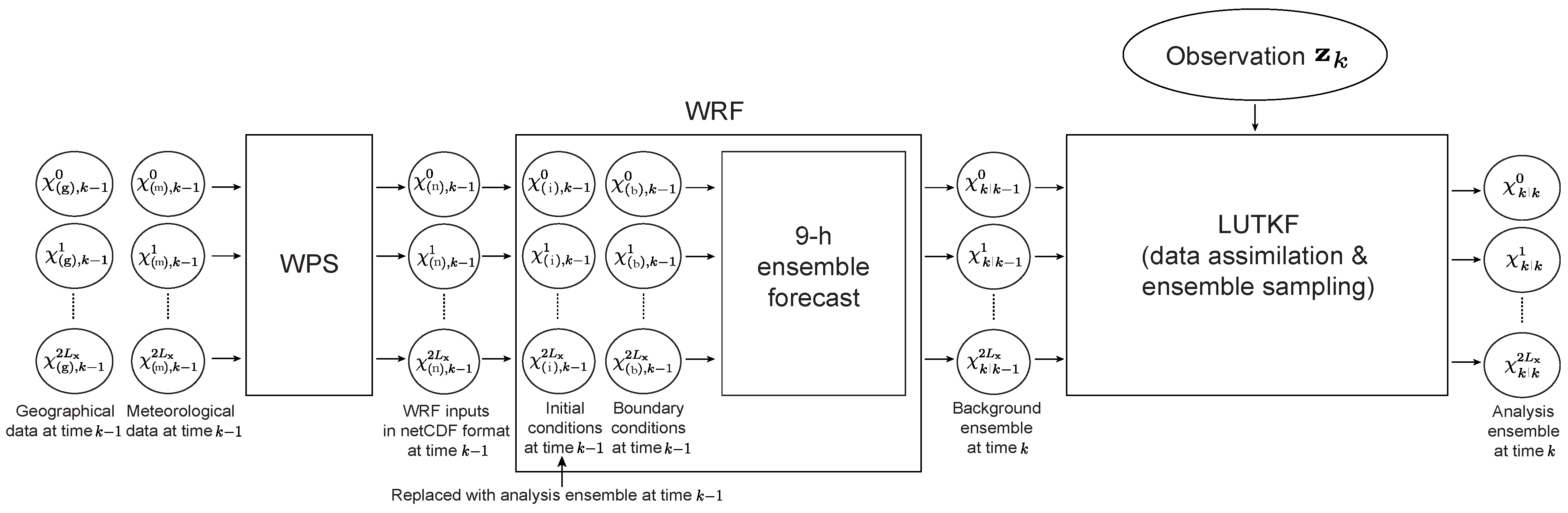
Figure 2.
Schematic design of the forecast and analysis cycle for the WRF-LUTKF system. Yellow star symbols represents the analysis time used for the data assimilation every 6 h (i.e., at 0000, 0600, 1200 or 1800 UTC). To perform the data assimilation at analysis time k (e.g., 0600 UTC) denoted by the yellow star symbol, the 9 h ensemble forecast using the WRF model generates the background ensemble every hour. The LUTKF computes the analysis ensemble by assimilating the hourly observations within seven time slots centered at analysis time k. To conduct the data assimilation at analysis time (e.g., 1200 UTC), several variables in the initial conditions for the 9 h ensemble forecast are substituted with their corresponding variables in analysis ensemble members .
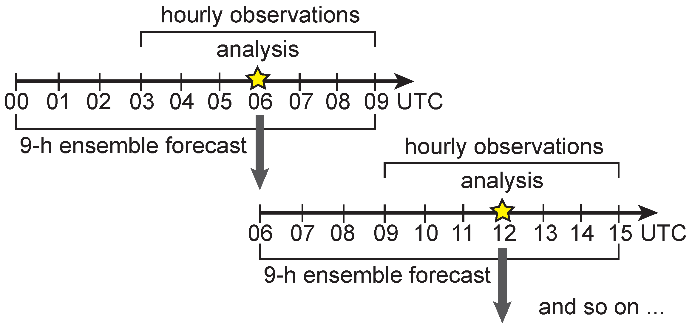
Figure 3.
Time series of prior domain-averaged RMSEs from the NCEP analysis for (a) 500 hPa zonal wind component (U500), (b) 500 hPa meridional wind component (V500), (c) 500 hPa temperature (T500), and (d) 500 hPa specific humidity (Q500) using the LETKF with , LETKF with , and LUTKF with . The blue shading represents that the LUTKF with a small ensemble size can provide better analysis results than the LEKTF, while the gray shading shows marginal estimation accuracy improvements of the LUTKF over the LETKF.

Figure 4.
Vertical profiles of the posterior mean bias relative to the NCEP analysis for (a) U, (b) V, (c) T, and (d) Q using LETKF with , LETKF with , and LUTKF with . The bias values are averaged over 13 days from 1200 UTC 6 September 2008 to 1200 UTC 19 September 2008.
Figure 4.
Vertical profiles of the posterior mean bias relative to the NCEP analysis for (a) U, (b) V, (c) T, and (d) Q using LETKF with , LETKF with , and LUTKF with . The bias values are averaged over 13 days from 1200 UTC 6 September 2008 to 1200 UTC 19 September 2008.

Figure 5.
As in Figure 4 but for the posterior mean spread and RMSE relative to the NCEP analysis. Solid lines represent the RMSE of the analysis ensemble mean for the LETKF and LUTKF against the NECP analysis. Dashed lines denote the spread of the analysis ensemble for the LETKF and LUTKF.
Figure 5.
As in Figure 4 but for the posterior mean spread and RMSE relative to the NCEP analysis. Solid lines represent the RMSE of the analysis ensemble mean for the LETKF and LUTKF against the NECP analysis. Dashed lines denote the spread of the analysis ensemble for the LETKF and LUTKF.
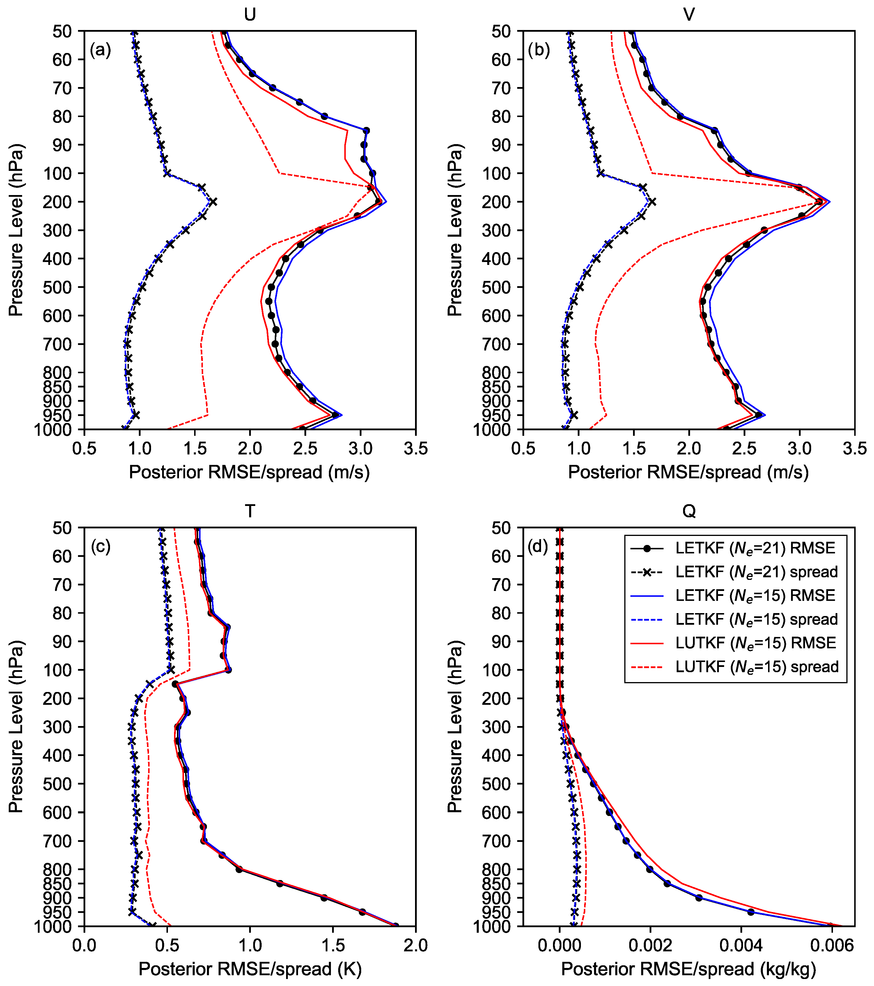
Figure 6.
As in Figure 4, but for the prior mean bias relative to the NCEP analysis for short-term (6 h) ensemble forecasts during 13 days from 1200 UTC 6 September 2008 to 1200 UTC 19 September 2008.
Figure 6.
As in Figure 4, but for the prior mean bias relative to the NCEP analysis for short-term (6 h) ensemble forecasts during 13 days from 1200 UTC 6 September 2008 to 1200 UTC 19 September 2008.
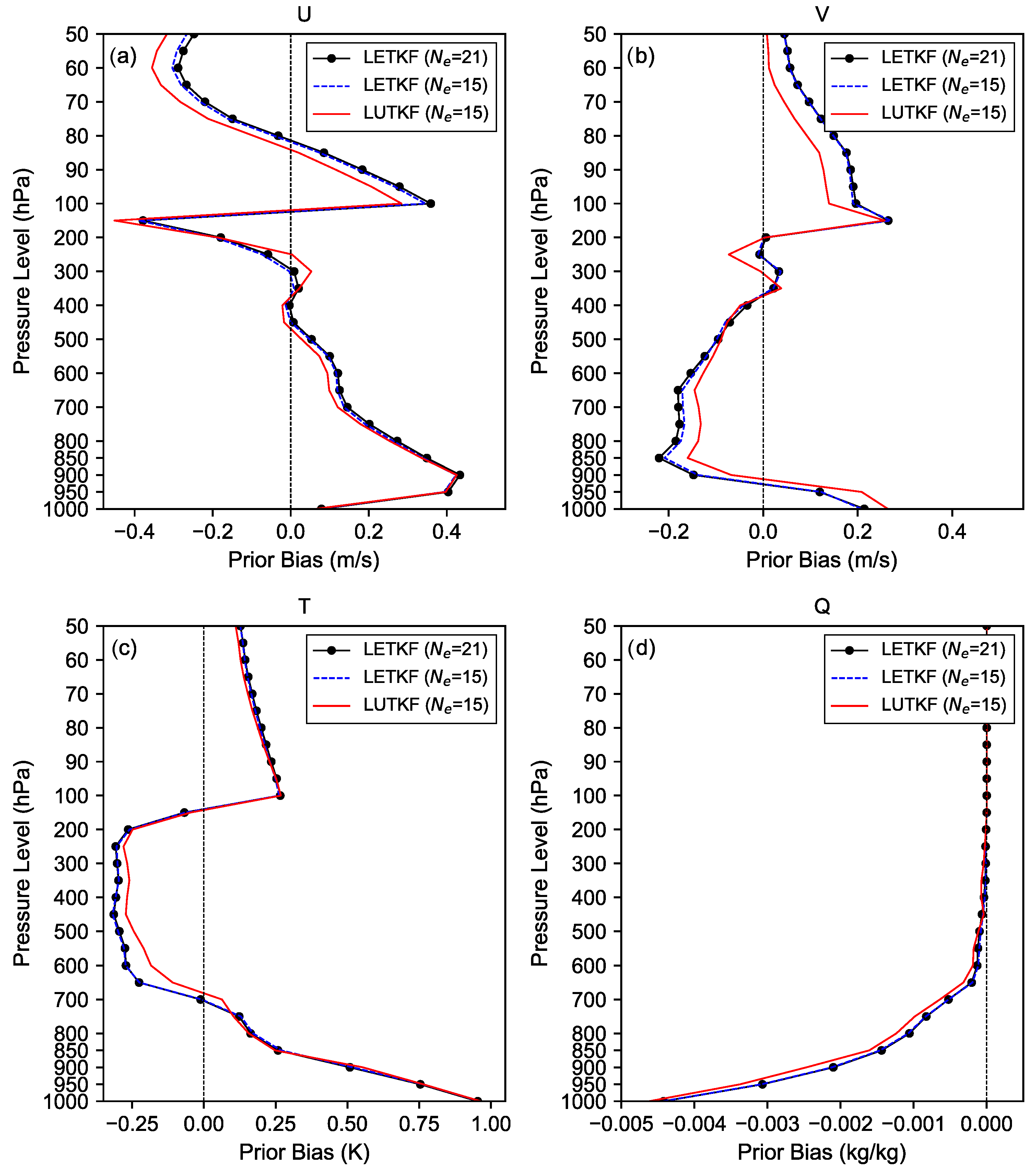
Figure 7.
As in Figure 5 but for the prior mean RMSE and spread of short-term (6 h) ensemble forecasts during 13 days from 1200 UTC 6 September 2008 to 1200 UTC 19 September 2008.
Figure 7.
As in Figure 5 but for the prior mean RMSE and spread of short-term (6 h) ensemble forecasts during 13 days from 1200 UTC 6 September 2008 to 1200 UTC 19 September 2008.
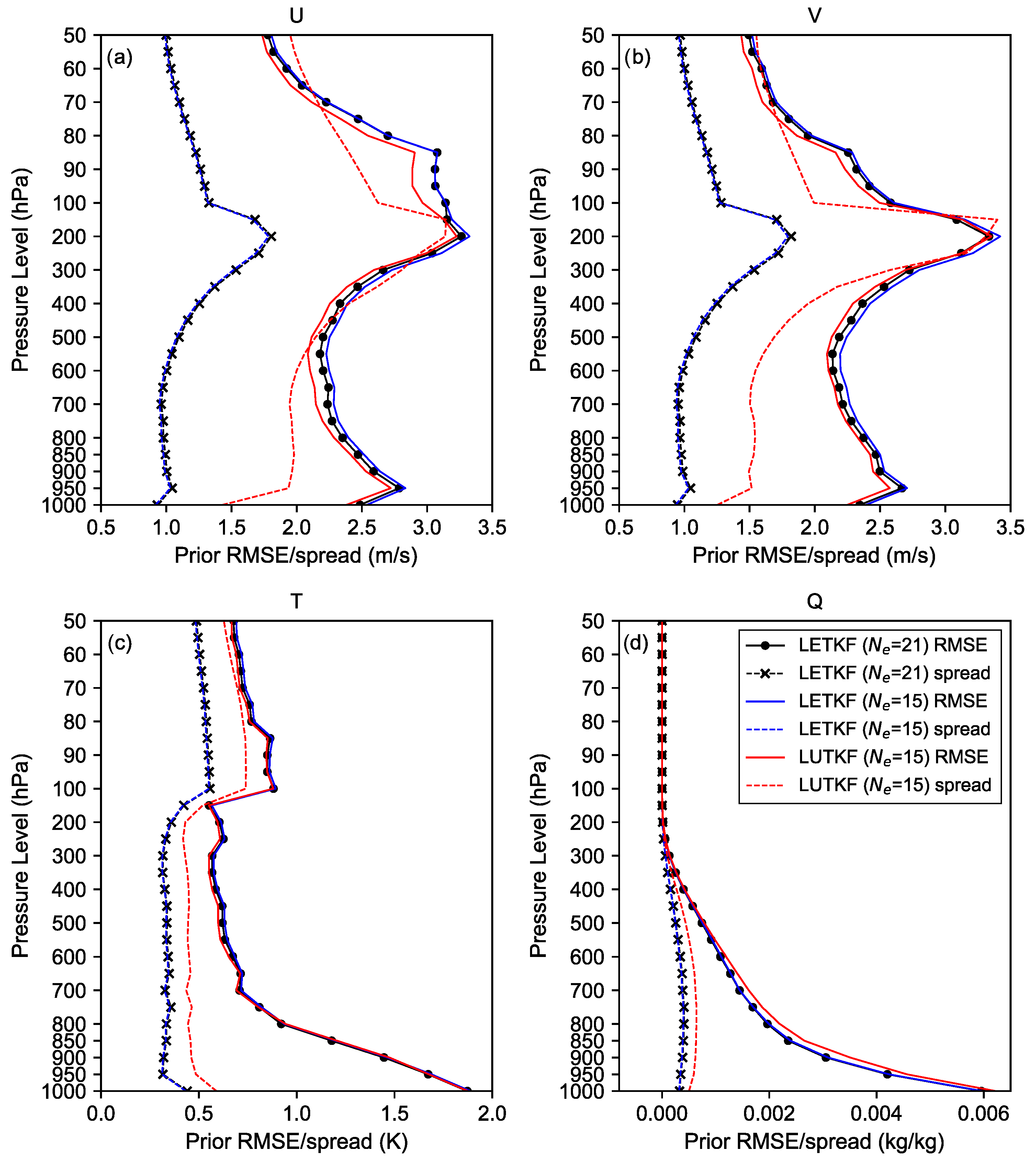
Figure 8.
Horizontal map of the mean sea level pressure (hPa) obtained from (a) NCEP analysis and the 6 h ensemble forecast initiated by the analysis of (b) LETKF with , (c) LETKF with , or (d) LUTKF with on 1200 UTC 12 September 2008.
Figure 8.
Horizontal map of the mean sea level pressure (hPa) obtained from (a) NCEP analysis and the 6 h ensemble forecast initiated by the analysis of (b) LETKF with , (c) LETKF with , or (d) LUTKF with on 1200 UTC 12 September 2008.
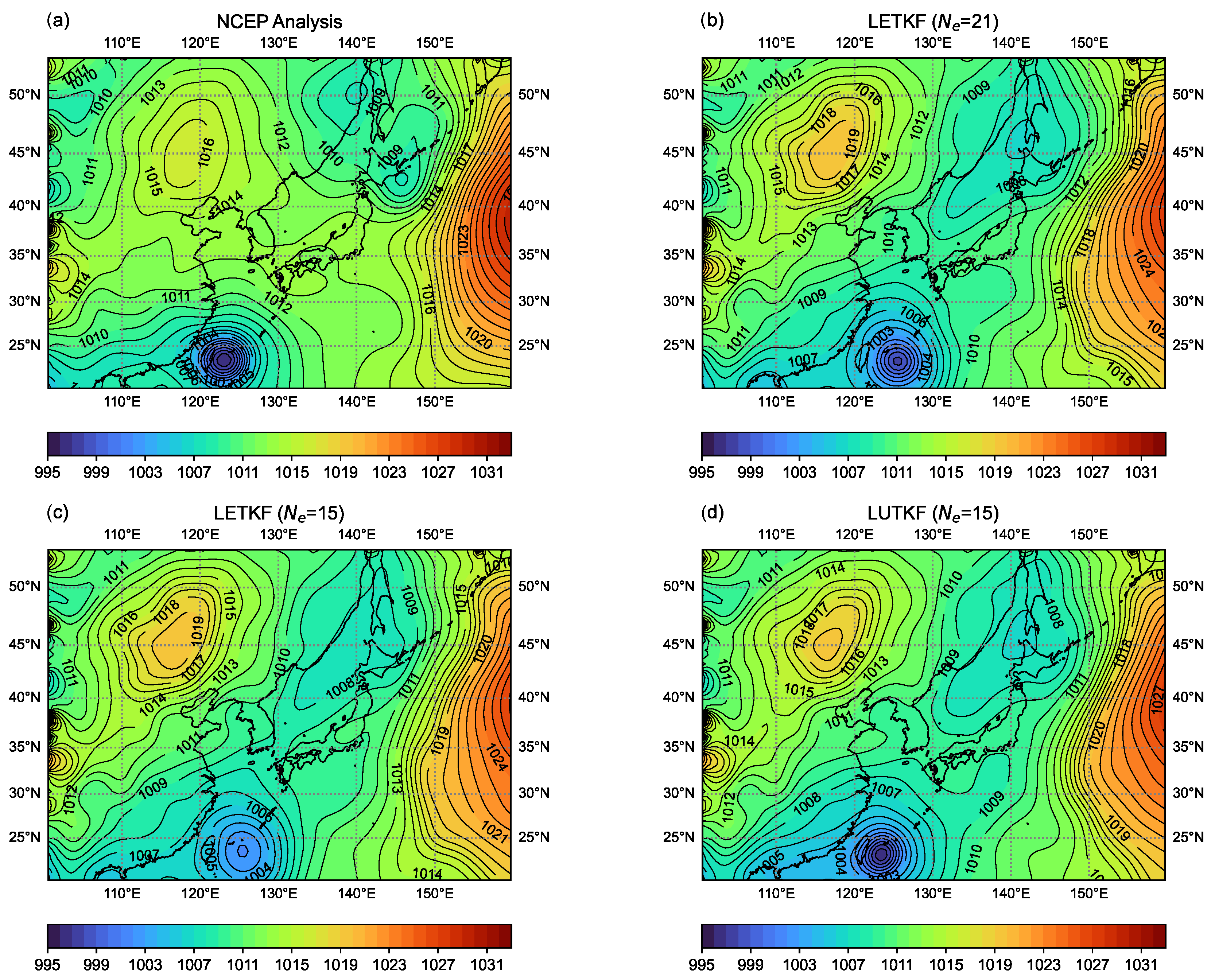
Figure 9.
As in Figure 8 but for the wind speed (m/s) at 850 hPa.
Figure 9.
As in Figure 8 but for the wind speed (m/s) at 850 hPa.
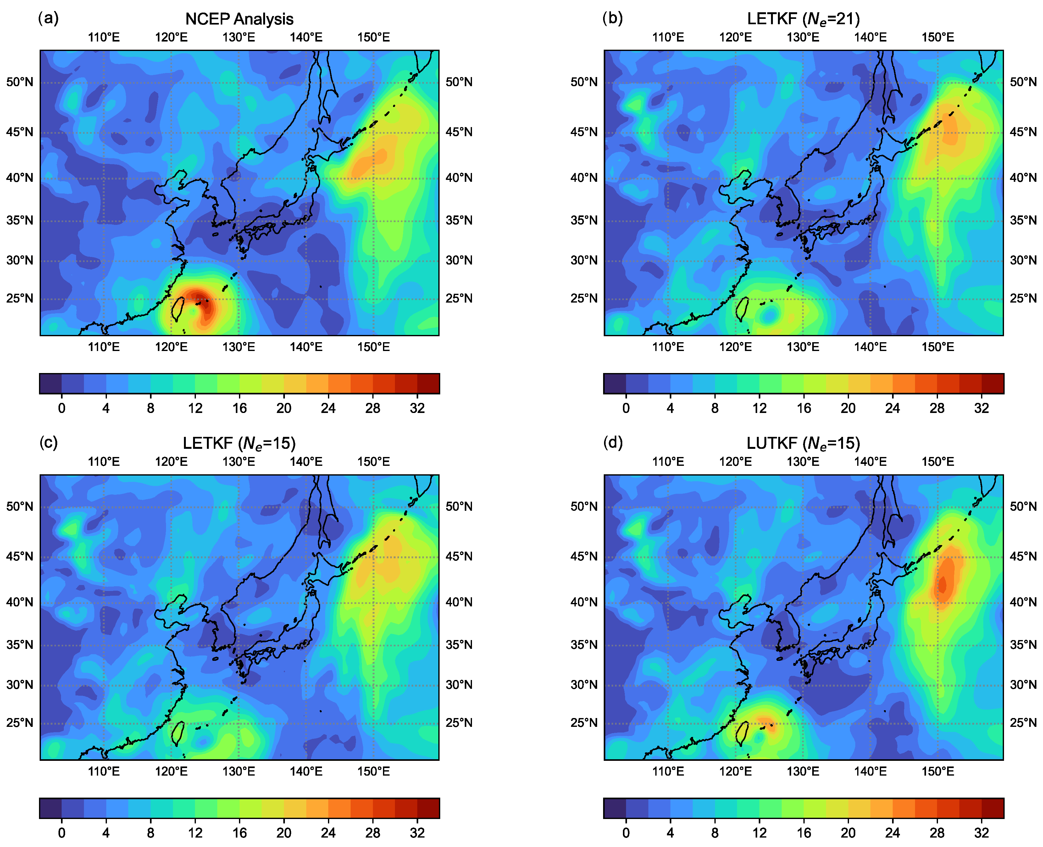
Figure 10.
Horizontal map of the difference of the 6 h forecast RMSE against the NCEP analysis between the LETKF with and LUTKF with for (a) zonal wind component (U500), (b) meridional wind component (V500), (c) temperature (T500), and (d) specific humidity (Q500) at 500 hPa during 13 days from 1200 UTC 6 September 2008 to 1200 UTC 19 September 2008. Red (blue) areas denote that the RMSEs of the LUTKF are smaller (larger) than those of the LETKF.
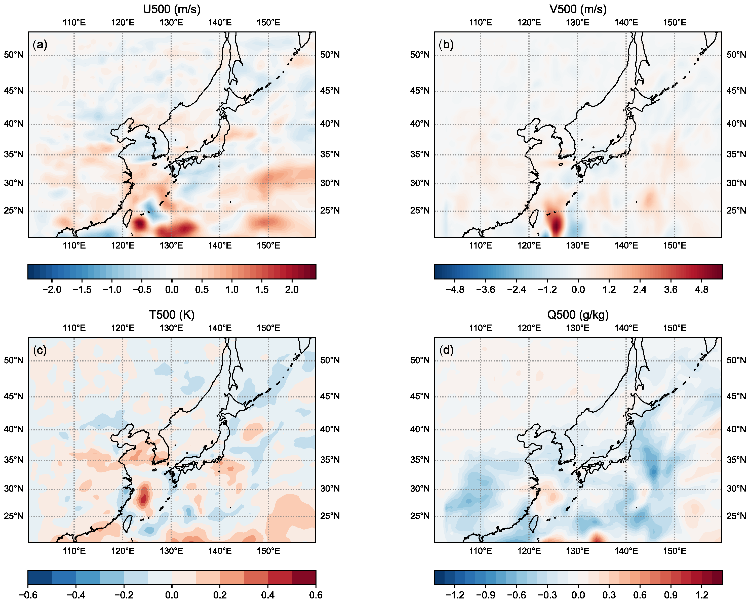
Figure 11.
As in Figure 10 but for the difference of the 6 h forecast RMSE between the LETKF with and LUTKF with .
Figure 11.
As in Figure 10 but for the difference of the 6 h forecast RMSE between the LETKF with and LUTKF with .


Table 1.
Prior mean RMSEs relative to observations for U, V, T, and Q using the LETKF with , LETKF with , and LUTKF with . The RMSE values are averaged over 13 days from 1200 UTC 6 September 2008 to 1200 UTC 19 September 2008.
Table 1.
Prior mean RMSEs relative to observations for U, V, T, and Q using the LETKF with , LETKF with , and LUTKF with . The RMSE values are averaged over 13 days from 1200 UTC 6 September 2008 to 1200 UTC 19 September 2008.
| Assimilation Method | U (m/s) | V (m/s) | T (K) | Q (kg/kg) |
|---|---|---|---|---|
| LETKF () | 3.86 | 3.86 | 1.95 | 174.56 |
| LETKF () | 3.91 | 3.93 | 1.99 | 179.47 |
| LUTKF () | 3.84 | 3.88 | 1.89 | 180.94 |
Table 2.
As in Table 1 but for posterior mean RMSEs relative to observations.
Table 2.
As in Table 1 but for posterior mean RMSEs relative to observations.
| Assimilation Method | U (m/s) | V (m/s) | T (K) | Q (kg/kg) |
|---|---|---|---|---|
| LETKF () | 3.38 | 3.34 | 1.75 | 124.03 |
| LETKF () | 3.48 | 3.45 | 1.80 | 129.19 |
| LUTKF () | 3.38 | 3.33 | 1.69 | 130.24 |
Table 3.
Computational time(s) of each assimilation method.
| Assimilation Method | 9 h Ensemble Forecast for the First Guess | Data Assimilation | Total |
|---|---|---|---|
| LETKF () | 148.45 | 17.36 | 165.81 |
| LETKF () | 75.68 | 14.58 | 90.26 |
| LUTKF () | 77.81 | 46.47 | 124.28 |
Disclaimer/Publisher’s Note: The statements, opinions and data contained in all publications are solely those of the individual author(s) and contributor(s) and not of MDPI and/or the editor(s). MDPI and/or the editor(s) disclaim responsibility for any injury to people or property resulting from any ideas, methods, instructions or products referred to in the content. |
© 2023 by the author. Licensee MDPI, Basel, Switzerland. This article is an open access article distributed under the terms and conditions of the Creative Commons Attribution (CC BY) license (https://creativecommons.org/licenses/by/4.0/).
Share and Cite
MDPI and ACS Style
Sung, K. The Local Unscented Transform Kalman Filter for the Weather Research and Forecasting Model. Atmosphere 2023, 14, 1143. https://doi.org/10.3390/atmos14071143
AMA Style
Sung K. The Local Unscented Transform Kalman Filter for the Weather Research and Forecasting Model. Atmosphere. 2023; 14(7):1143. https://doi.org/10.3390/atmos14071143
Chicago/Turabian StyleSung, Kwangjae. 2023. "The Local Unscented Transform Kalman Filter for the Weather Research and Forecasting Model" Atmosphere 14, no. 7: 1143. https://doi.org/10.3390/atmos14071143
Note that from the first issue of 2016, this journal uses article numbers instead of page numbers. See further details here.