Abstract
The study investigated the impact of temperature extremes on carbon emissions (CE) from crop production. (1) Background: Many scholars have studied climate extremes. However, the research on the relationship between temperature extremes and CE is not extensive, which deserves attention. (2) Methods: The study adopted a fixed-effect model to analyze the impact of temperature extremes on CE from crop production, and the moderating effect was tested using total factor productivity (TFP) in agriculture. (3) Results: Temperature extremes in Hebei Province were mainly reflected in a decline in the cold day index (TX10p) and a rise in the warm spell duration index (WSDI) and the number of summer days (SU25). Additionally, TX10p was positively correlated with CE. For every 1% reduction in TX10p, CE dropped by 0.237%. There was no significant correlation between WSDI and CE. Finally, the agricultural TFP had a significant moderating effect on CE, with each 1% increase resulting in a corresponding 0.081% decrease in CE. (4) Conclusions: The results indicated a warming trend in Hebei Province, which resulted in a decrease in the number of winter days, and reduced CE from crop production. The improvement of input efficiency in agricultural production factors helped moderate the CE.
1. Introduction
There have been frequent temperature extremes caused by climate change in recent years, which have already received widespread attention from the international community [1]. Many available studies that focused on climate extremes found that agriculture is significantly affected by changes in climate [2]. Some scholars pointed out that farmers and governments take actions to mitigate the impact of climate extremes on crop production, such as increasing fertilizer and pesticide use and promoting agricultural machinery upgrades. These actions lead to changes in carbon emissions (CE) from crop production. For example, the excessive use of fertilizers and pesticides can increase additional CE, while intensive agricultural machinery upgrades have the opposite effect [3,4,5]. Therefore, agricultural CE could be severely affected by climate extremes, because the inputs of carbon sources related to crop production will change to cope with the extremes. It has become an international topic to study the impact of climate extremes on crop production CE, and strengthen the construction of green agriculture [6].
Numerous researchers have investigated the frequency and intensity of climate extremes and analyzed the potential future trends. Research by Anemüller et al. illustrated that the climate extremes in most land areas were mainly reflected in a significant decrease in the frequency of cold nights and a significant increase in the frequency of warm nights [7]. Jiao et al. obtained similar results to Anemüller et al., and indicated that the warm index and the index of temperature extremes were increasing, while the cold index and the index of daily temperature range were decreasing in northern China [8]. However, there was no significant extreme precipitation compared with extreme temperature in northern China, because the northeast wind there was restricted, which was not conducive to water vapor transportation [9]. Meanwhile, a study showed that changes in temperature had more dramatic effects than changes in precipitation [10], making the impact of temperature extremes on CE from crop production more important. Temperature extremes have continued to occur in China over the past 50 years, mainly manifesting as an increase in the frequency of warm extremes and a decrease in the frequency of cold extremes [11,12], especially in Hebei, Sichuan, Hubei, where temperature extremes were more significant than in other places [13]. Since crop production is highly dependent on the amount of cultivated land, temperature extremes in Heilongjiang, Henan, Shandong, Inner Mongolia, and Hebei, which are the top five provinces in China [14], were more valuable for research. The province that satisfied the conditions of both a large cultivated land area and temperature extremes is Hebei. Therefore, this study focused on the impact of extreme temperatures on CE in Hebei Province, China.
Studies on agricultural CE have made considerable progress. The carbon emission coefficient method has been widely used as a calculation method for measuring agricultural CE in many studies [15,16,17]. Some scholars used carbon emission coefficients to calculate Chinese CE and conducted driving factor analysis using the Logarithmic Mean Divisia Index (LMDI) model [18]. Furthermore, some scholars pioneered the use of the life cycle assessment method [19], ecosystem Lund–Potsdam–Jena model [20], and remote sensing technology [21] for agricultural CE measurement. Fertilizer application [22], straw burning [23], and irrigation [24] were factors that directly affected the carbon emission levels of crop production. In addition, agricultural development level, industrial structure, labor force level [25], improvements in agricultural production efficiency, research, development expenditure, government efficiency [26], and digital economic development [27] also had significant impacts on CE.
As climate extremes increase in frequency, climate factors are gradually becoming an undeniable factor influencing agricultural CE [28]. Climate extremes have not only led to increased input of production factors by affecting crop growth with drought and pest infestations [29], but have also harmed carbon absorption in land systems [30]. Strengthening agricultural management and changing production methods are effective ways to mitigate climate extremes [31]. There are several ways to make agriculture more adaptable to climate extremes and improve the input efficiency of production factor, while reducing CE, such as agricultural machinery upgrades [3], improving fertilizers and water sources [32], soil management to improve the carbon sequestration capacity of cultivated land [33], and the use of soil microbial response mechanisms to various climate changes [34]. The use of multiple crop rotations and intercropping can also alleviate the effects of high temperatures and droughts by maintaining soil moisture, thereby reducing CE caused by irrigation energy consumption [35]. However, some studies also found that climate extremes did not necessarily lead to an increase in CE. For example, extreme high temperatures in Switzerland reduced pesticide use by 11.5%, with a subsequent reduction in CE caused by pesticide use [36]. Similarly, research in Hebei Province found that local climate extremes were related to low-carbon agricultural efficiency, and temperature and precipitation had a positive impact [37].
The various measures mentioned above, such as upgrading agricultural machinery, improving fertilizers, water-saving irrigation, rational use of pesticides, and adopting new planting methods, are all aimed at optimizing production factor input efficiency to reduce carbon source usage, while mitigating the pressure of climate extremes on CE. Agricultural total factor productivity (TFP) is a common indicator for measuring agricultural production factor input efficiency and a specific manifestation of the development of agricultural productivity [38]. There have been some indications that the continuous improvement of TFP promotes the transformation of the agricultural development mode, gradually changing from extensive to intensive [39]. Long-term adjustments to production factors such as fertilizers and machinery could improve agricultural environmental adaptability to reduce CE [40].
The above studies showed that climate extremes, particularly temperature extremes, influence agricultural CE from crop production. However, research on the relationship between them within the context of the current increasingly severe temperature extremes has not been extensive. How do temperature extremes affect CE from crop production? Could the current crop production models effectively bear out the CE changes brought about by significant temperature extremes? These are matters of great concern for ensuring food security and agricultural economic stability. Based on previous research findings, this study focused on Hebei Province as the research subject, because it is the only province in China that satisfies two conditions: it is among the top five provinces in China in terms of arable land area and has already experienced temperature extremes. For research purposes, this study used extreme temperature indices to study the relationship between temperature extremes and CE from crop production in Hebei Province, China. Then, TFP was introduced as a moderating variable to analyze whether changes in the input efficiency of production factors could moderate the CE changes caused by temperature extremes.
2. Material and Methods
2.1. Study Area
Hebei Province is located in the North China Plain (36°05′ N–42°40′ N, 113°27′ E–119°50′ E) (Figure 1a), with a total area of 188,800 km2, surrounding Beijing and Tianjin, and is divided into 11 prefecture-level cities. Due to its four-seasonal climate and geographical location, Hebei Province has become an important crop-producing area in China and an important promotion area for China’s East–West Economic Belt. According to the Hebei Rural Statistical Yearbook, the main crops in Hebei Province include rice, wheat, corn, millet, soybeans, potatoes, sweet potatoes, etc. This study focused on the CE of these crops. The mean temperature in January is below 3 °C, and in July it ranges from 18 °C to 27 °C. The mean annual temperature (MAT) is approximately 12 °C (Figure 1b). The MAT is slowly rising, excluding the marked decline between 2010 and 2013.
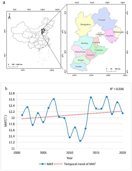
Figure 1.
Location and temperature conditions of Hebei Province. (a) The location of Hebei Province, China. (b) The temporal trend in mean annual temperature (MAT) from 2001 to 2020.
2.2. Data Description
The research period was from 2001 to 2020. Based on research needs, this study selected temperature data, CE factors consumption of crop production data, and other CE-related factors data in 11 prefecture-level cities in Hebei Province. The temperature data used in this study were supplied by the China Meteorological Science Data Sharing Service [41]. The original data were daily site data, and the sites were distributed in various parts of Hebei Province. The following steps were used to obtain daily temperature data of prefecture-level cities, covering all areas of the city: (1) The original data were cleaned using Python to retain the values of latitude, longitude, and average daily temperature. (2) The exhibition points were reprojected, and the daily data were interpolated using the inverse distance weighting method. (3) According to the administrative division, the data were divided into statistics and stitched together to obtain the daily temperature data of each city. CE factors consumption of crop production data and other CE-related factors data came from the Hebei Rural Statistical Yearbook from 2002 to 2021 [42].
2.3. Data Processing
2.3.1. Calculation of Climate Indexes
This study referred to the extreme climate indexes set by the 10 Expert Team on Climate Change Detection and Indices [43] to measure temperature extremes. Jiang and Kim et al. both used these indexes to conduct extreme climate researches [44,45]. Rclimdex1.0 is used to analyze the quality of the temperature data of cities and calculate 12 extreme temperature indexes of 11 prefecture-level cities, which were classified into three categories, namely relative threshold, absolute threshold, and extreme value [46] (Table 1).

Table 1.
Extreme temperature indexes and definitions.
The Theil–Sen slope is a non-parametric estimation method, which is often used to analyze the changing trend in a certain element in a long-term series [8]. Its calculation formula is as follows:
In this formula, median represents the median function; β represents the changing trend of an extreme temperature index; xi and xj represent the sequence data of different years; ti and tj represent the time series. When β > 0, it indicates that an extreme temperature index is rising; when β < 0, the index shows a downward trend.
In the process of calculating the extreme temperature indexes, the significance degree of the index can be obtained. Based on these, this study selected the extreme temperature indexes required in future research. The more cities in which an extreme temperature index is significant, the wider is the impact range of extreme temperature changes represented by the index. This index also has broader implications for crop production and is an ideal index to represent temperature extremes in Hebei province. To determine the most effective indexes, the number of prefecture-level cities with a significant extreme temperature index were counted, and the results are shown in Figure 2.
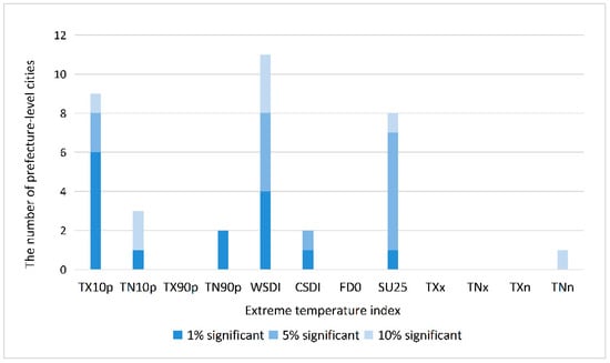
Figure 2.
The number of cities whose extreme temperature index passed the significance test.
From the figure, it can be seen that SU25, TX10p, and WSDI had significant changes in most prefecture-level cities in Hebei Province. Among them, SU25 is an absolute threshold index reflecting the extreme high temperature of summer; WSDI is a relative threshold index reflecting the same content; and TX10p is a relative threshold index reflecting the extreme coldness in winter. Both SU25 and WSDI are extreme temperature indexes for high temperature phenomena in summer, but the threshold types are different. Therefore, only one of them was selected. This study discarded SU25 and took TX10p and WSDI as variables in the regression to measure extreme temperature changes in Hebei Province. There were two reasons for this: (1) TX10p, like WSDI, belongs to the relative threshold index, indicating that that Hebei Province mainly experienced relative changes. (2) Judging from the number of prefecture-level cities with significant changes, TX10p is larger than SU25, and the scope of the influence of TX10p is wider.
2.3.2. Calculation of Carbon Emissions
Many scholars believe that the CE from crop production is largely derived from the input production factors brought by the main agricultural activities. These input production factors are generally considered to be the CE factor [18,47]. Hence, this study selected six CE factors and employed the Intergovernmental Panel on Climate Change (IPCC) carbon emission coefficient method, which has been widely adopted by researchers to calculate the CE from crop production [48]. According to the emission coefficient of CE factors released by Chinese and foreign laboratories, an assessment of CE from crop production was conducted (the emission coefficient of the six major CE factors multiplied by the consumptions of these CE factors). A comprehensive breakdown of each carbon emission coefficient along with their respective sources is presented in Table 2.
Table 2.
Carbon emission factors from crop production, coefficients, and sources.
The estimation formula of CE from crop production is:
A set of variables was introduced to calculate CE. E represents the total CE from crop production; i in the subscripts of Ei, Ti, and Ki represents the ith of the six CE factors; Ei represents the CE from crop production associated with the ith CE factor; Ti is used to represent the input amount of the ith CE factor; Ki represents the carbon emission coefficient of the ith CE factor.
Utilizing Formula (2), we calculated the panel data of the annual CE of 11 prefecture-level cities, by adopting the CE factors data from the Hebei Rural Statistical Yearbook from 2002 to 2021. The CE factors are listed in Table 2. These data of CE factors were obtained from the annual inputs of fertilizers, pesticides, agricultural films, diesel, plowing, and irrigation for crop production in 11 prefecture-level cities in Hebei Province, which were disclosed in the Hebei Rural Statistical Yearbook. Next, these panel data of CE calculated by Formula (1) were used as dependent variables in the Formulas (3)–(5) to study the impact of temperature extremes on CE.
2.4. Research Methods
2.4.1. Fixed Effect Model
The study design drew on the model setting ideas advanced by other scholars [50], designed the main model as a fixed effect estimation model of panel data [51], and selected control variables with reference to the research of Tian et al. [18], as follows:
In the formula, Cit represents the CE from crop production and serves as the dependent variable of the model after taking the logarithm; i represents prefecture-level cities in Hebei Province; t is the time interval; αi represents the individual effect of each city, and λt represents the time effect; TX10pit and WSDIit take the logarithm as the core dependent variables, which are used to reflect the extreme temperature changes in prefecture-level cities in Hebei Province; EIit, CIit, SIit, and LABit are model control variables; εit is a random disturbance item, and βj (j = 1, 2, 3, 4, 5, and 6) is a parameter to be estimated.
The selection of control variables was based on the Kaya identity, which was formally proposed at the IPCC International Symposium [52]. Since then, the method of using the LMDI factor decomposition method has been commonly used to decompose the influencing factors of CE. Based on the Kaya identity [53], the study used the following factors as the control variables affecting agricultural CE: (1) agricultural efficiency (EI), which is the ratio of the total CE from crop production to the total output value of crops; (2) agricultural structure (CI), which is the ratio of the total output value of crops to the total output value of agriculture, forestry, animal husbandry, and fishery; (3) agricultural economic level (SI), which is the ratio of the total output value of agriculture, forestry, animal husbandry, and fishery to the scale of agricultural labor; and (4) the scale of agricultural labor (LAB), which is the total workforce engaged in agriculture, forestry, animal husbandry, and fishery.
2.4.2. Fixed Effect Test
Before the empirical analysis could be performed, it was necessary to test whether there were serial correlations and heteroscedasticity in the variables. The results showed that there were serial correlations and heteroscedasticity in the disturbance term; therefore, it was necessary to use an appropriate estimation method to remove these influences from the regression analysis. The outcome of the test is shown in Table 3.
Table 3.
Serial correlation and heteroscedasticity test results.
It was essential to determine the suitability of a fixed effect model. The null hypothesis was proposed as H0: pool model, and the individual fixed effect test was carried out. When performing the individual fixed effect test, F = 50.907 was greater than the critical value 2.341, corresponding to the 5% significance level. Therefore, there was an individual effect to reject the null hypothesis pool model. The LR test result was 125.254, which was far greater than the critical value of 30.144, corresponding to the 5% significance level of the chi-square test, which also rejected H0. Furthermore, the time point fixed effect test was carried out and the test result F = 34.220 was greater than the critical value 2.054, corresponding to the 5% significance level. Additionally, the LR test statistic was 160.740, greater than the critical value 18.307 and corresponding to the 5% significance level of the chi-square test, which also rejected H0. There was therefore a double fixed effect of individual time point. Finally, it was necessary to verify whether there were double fixed effects of individual time points instead of random effects. The null hypothesis was a random effects model. Due to the existence of serial correlation and heteroscedasticity, the modified Hausman statistic was used with a result of Prob > chi2 = 0.000, which significantly rejected the null hypothesis, indicating that there was a fixed effect.
2.4.3. Moderating Effect Model
As evidenced by previous research mentioned in the Introduction, temperature extremes can affect the input of agricultural production factors, subsequently influencing CE from crop production. Fortunately, enhancing the input efficiency of production factors could have offered an effective means of mitigating the CE change caused by temperature extremes. Agricultural TFP is a common indicator for measuring input efficiency of agricultural production factors. This study attempted to validate the moderating effect of TFP on crop production. To this end, this study referenced research of Dong et al. and added an interaction term to the two independent variables based on Formula (3) [50], which incorporated the intersection of agricultural TFP and extreme temperature indexes, and applied a series of formulas to test their efficacy:
Since there were two independent variables reflecting extreme temperature changes, the moderating effect was divided into two formulas. Formula (4) tested the moderating effect of input efficiency of agricultural production factors on the duration of cold days in winter, and Formula (5) tested the moderating effect of input efficiency of agricultural production factors on the duration of hot days in summer.
In these formulas, TFP is the agricultural TFP, which was used to assess the input efficiency of agricultural production factors. The higher the efficiency, the more advanced the agricultural production mode and the less influence extreme temperature changes had on CE. The value of TFP was the fixed reference Malmquist index under the assumption of constant returns to scale. The output index utilized the gross value of agricultural production, while the input indexes utilized labor force, chemical fertilizer, irrigation and planting area, diesel oil, and agricultural film usage in each city. The cross-product coefficients δ3 and θ3 are utilized in quantifying the moderating effect of agricultural TFP on the relationship between temperature extremes and CE.
2.5. Variable Descriptive Statistics
Before carrying out the test of fixed effects and moderating effects, descriptive statistics were performed on all variables, and the statistical results are shown in Table 4.
Table 4.
Variable descriptive statistics.
3. Results
3.1. Changes in Extreme Temperature Indexes
3.1.1. Cold Days
Through an analysis of temperature data collected from prefecture-level cities in Hebei Province over the years 2001 to 2020, it was determined that the annual variation in extreme temperature was mainly reflected in three indexes: TX10p, WSDI, and SU25. Among them, TX10p quantifies the number of days on which the highest temperature falls below the 10th percentile, mainly indicating the duration of winter with low temperatures during the day. It could also be said that TX10p can represent the length of cold winter days to a certain extent. Compared with TN10p, which measures the duration of winter using the low temperatures at night, TX10p was more valuable in this study. Because daytime is the main period for crop photosynthesis and growth, daytime temperature changes have a greater impact on crop growth. Moreover, there was a statistically significant change in TX10p in most cities, so focusing on the analysis of the changes in TX10p explained the extreme temperature changes in Hebei Province in winter.
TX10p showed significant changes in nine prefecture-level cities in Hebei Province. Among them, Shijiazhuang, Handan, Baoding, Cangzhou, Langfang, and Hengshui all reached the 1% significance level. As shown in Figure 3, the extreme temperature index TX10p of these six cities decreased at rates of 0.38 d/a, 0.352 d/a, 0.405 d/a, 0.375 d/a, 0.394 d/a, and 0.351 d/a, respectively. A reduction in TX10p indicates a reduction in the number of days during winter, while an escalation indicates a rise in the number of days during winter. The outcome revealed that Hebei Province had encountered a decline in cold days, thereby eliciting the phenomenon of a “warm winter”. The other three prefecture-level cities reached a significant level of at least 10%, following the same trend. It could be considered that most areas in Hebei Province have experienced a warming trend in winter.
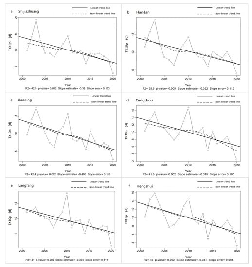
Figure 3.
Change trend in the Cold Days Index (TX10p) in prefecture-level cities. (a) Shijiazhuang, (b) Handan, (c) Baoding, (d) Cangzhou, (e) Langfang, and (f) Hengshui.
3.1.2. Warm Spell Duration Index
WSDI refers to the number of days on which the highest temperature was over the 90th percentile, and measures the number of days with continuously high temperatures in summer. All prefecture-level cities in Hebei Province experienced significant changes in this index: four prefecture-level cities reached a 1% significance level, four prefecture-level cities reached a 5% significance level, and three prefecture-level cities reached a 10% significance level. Figure 4 shows the changing trend of WSDI in eight prefecture-level cities with a minimum 5% significance level, including Shijiazhuang, Tangshan, Qinhuangdao, Handan, Xingtai, Baoding, Langfang, and Hengshui. The WSDI of these eight cities increased at rates of 0.665 d/a, 0.675 d/a, 0.704 d/a, 0.522 d/a, 0.494 d/a, 0.600 d/a, 0.700 d/a, and 0.518 d/a, respectively. It can be seen from the figure that the WSDI has risen sharply in various cities since 2016, indicating that the duration of high temperatures during summer demonstrated a significant rise in most parts of Hebei.
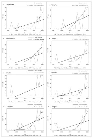
Figure 4.
Change trend of Warm Spell Duration Index (WSDI) in prefecture-level cities. (a) Shijiazhuang, (b) Tangshan, (c) Qinhuangdao, (d) Handan, (e) Xingtai, (f) Baoding, (g) Langfang, and (h) Hengshui.
Combining Figure 3 and Figure 4 with the above analysis content, it was determined that since 2001, most areas in Hebei Province had experienced extreme temperature changes, mainly manifested in the shortening of the duration of winter with low temperatures represented by TX10p, and the length of the duration of summer with continuously high temperatures represented by WSDI. It was also found that both have relatively large slopes, indicating that the extreme climate phenomena represented by these two indexes underwent relatively large changes. However, there were differences between the two. TX10p fluctuated and fell with a slope of about 0.35 d/a. WSDI rose rapidly from around 2016 with a slope of about 0.6 d/a.
3.2. Carbon Emissions from Crop Production
Figure 5 is a statistical chart of the total CE from crop production in Hebei Province from 2001 to 2020. The total CE from crop production rose rapidly from 2001 to 2007, and reached its peak at 7.897 million tons in 2007. After 2007, the total CE showed a downward trend and began to decline rapidly in 2016. By 2020, the CE reached the lowest level during the study period at 5.393 million tons. In 2004, there was a notable surge in the growth rate of CE. The growth rate of CE reached the highest value of 19.88% in 2004, gradually began to appear negative after 2006, and reached the lowest value of −11.46% in 2008, and then remained at a low level.
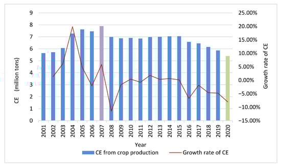
Figure 5.
Carbon emissions (CE) and the growth rate of CE from crop production in Hebei Province from 2001 to 2020.
Since 2000, Hebei Province vigorously developed agriculture and pursued economic growth, which directly led to an increase in CE. Zhou et al. pointed out that in the process of pursuing agricultural economic growth, the degree of mechanization, the intensity of chemical fertilizer application, and energy consumption were all important factors that caused the increase in agricultural CE in Hebei Province [54]. Therefore, the rise in CE from 2000 to 2007 was related to the low utilization rate of production factors under the extensive production mode. In 2007, Hebei Province accelerated the pace of low-carbon agriculture, implemented the “Double Thirty” project, and promoted low-carbon economic and technological reforms [55]. The growth rate of CE had gradually turned negative, and the total amount of CE remained in balance for a period. Especially after 2016, China paid more attention to green agricultural production and ecological sustainable development. The specific measures such as zero growth in chemical fertilizer use were implemented, and CE began to show a clear downward trend.
3.3. Agriculture Total Factor Productivity
It is generally believed that the higher the agricultural TFP is, the more scientific and efficient the input method of agricultural production factors will be. Agricultural TFP was used as the moderating variable of the model, and descriptive statistics research was needed for it. According to the agricultural TFP of Hebei Province from 2001 to 2020 (Figure 6), during 2001 to 2004, the agricultural TFP remained below 1. It increased significantly after 2005, and reached its first peak of 1.289 in 2008. Since 2008, it has remained between 1 and 1.2. From 2016 to 2020, with the continuous advancement of agricultural modernization technology, the agricultural TFP once again achieved a breakthrough, reaching a peak of 1.304 in 2020. Overall, the agricultural TFP of Hebei Province experienced rising fluctuations.
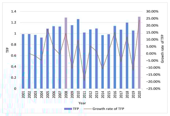
Figure 6.
Agricultural total factor productivity (TFP) and the growth rate of TFP in Hebei Province from 2001 to 2020.
3.4. Temperature Extremes and Carbon Emissions
The objective of this study was to investigate the effects of temperature extremes on CE from crop production in Hebei Province. Regression analysis of the individual time-point double fixed effect model was carried out to obtain the results shown in Table 5. In order to ensure the robustness and predictability of the regression results, six model processing methods in Table 5 were adopted:
Table 5.
Fixed effect regression results.
Model 1: Direct regression of the dependent variable and the independent variable, to observe whether there is a direct relationship between the two.
Model 2: Ordinary least squares (OLS) is a basic parameter estimation method that estimates the unknown parameters of a linear regression model by minimizing the sum of squared residuals.
Model 3: Least squares dummy variable (LSDV) is a method for working with panel data. The LSDV method introduces dummy variables (also known as fixed effects) based on OLS to control individual fixed effects.
Model 4: Model 4 combines LSDV with robust standard errors for robust estimation. Robust standard error is a modified standard error estimation method that better handles heteroscedasticity or correlation in the data. Combining LSDV with robust standard errors increases the robustness of the LSDV and reduces the impact of outliers or violations of model assumptions on parameter estimates.
Model 5: Panel-corrected standard errors (PCSE) is a better fixed effect model than the LSDV. Unlike the LSDV, which controls individual fixed effects by introducing dummy variables, the PCSE corrects all possible serial correlations and heteroscedasticity using a heteroscedasticity processing method to obtain a more robust estimate of the standard error.
Model 6: The corresponding random effect result serves as a reference for comparative analysis.
According to the regression results in Table 5, the following results were obtained from the core independent variable: the coefficient of the core independent variable lnTX10p was 0.237, and passed the significance test at the confidence level of 1%. This showed that in Hebei Province, for every 1% decrease in the index TX10p representing the duration of winter cold, CE from crop production would decrease by 0.237%. Another core independent variable, lnWSDI, had a coefficient of −0.047, but was not statistically significant. This showed that the index WSDI representing the duration of continuous high temperature in summer, had little effect on CE. Based on the previous analysis of changes in extreme temperature indexes from 2001 to 2020, it was concluded that the duration of cold days in winter had shortened in the past two decades, leading to a decline in CE from crop production.
Additionally, there was a noteworthy positive correlation between the CE from crop production and the control variables, such as EI, CI, and SI. For every incremental ton/yuan in agricultural efficiency, there was a corresponding 0.706% increase in CE; for every incremental 1% in agricultural structure, there was a corresponding 0.943% increase in CE; and for every incremental 1 yuan/person in agricultural output levels, there was a corresponding 0.050% increase in CE. There was no notable outcome to support a correlation between LAB and CE.
3.5. The Moderating Effect of Agriculture TFP
Since WSDI in the fixed effect model was not significant, only the result of Formula (4) is discussed here to analyze the moderating effect (Table 6). The result showed that the coefficient of the interaction term was 0.318, and it passed the significance test at the 5% confidence level. This indicated that agricultural TFP could significantly and positively regulate the relationship between TX10p and CE. With every 1% increase in TFP, the impact of TX10p on CE increased significantly by 0.318%. As the duration of low temperature in winter in Hebei Province became shorter, the CE decreased accordingly, and the higher the TFP, the more effectively the climatic conditions were utilized, further reducing CE.
Table 6.
Moderating Effect Regression Results.
4. Discussion
Most previous studies on the relationship between climate extremes and crop production focused on the changes brought about by climate extremes on agricultural production methods [31] and production factor inputs [29,35], and simply speculated that these changes may affect CE. There were few studies that could directly use empirical data to prove the impact of climate extremes on CE of crop production. Based on previous studies, this study used extreme temperature indexes and CE data from Hebei Province between 2001 and 2020 to visually verify that TX10p had a significant positive impact on the CE from crop production: the shorter the cold duration in winter, the lower the CE. Simultaneously increasing TFP could enhance the effective use of climate change. These findings provided an important reference for Chinese agriculture to improve the input efficiency of agricultural production factors under changing climate conditions, make rational use of climate change, and realize green agriculture.
4.1. Impact of TX10p on Carbon Emissions
The results of this study may not be consistent with the views of some scholars, who believe that rising temperatures will cause the greenhouse effect, making it difficult for crops to grow and requiring more CE factors to maintain normal crop production [30,56]. However, this is not necessarily true in all regions. Other studies showed that rising temperatures lead to lower CE [36,37]. Hebei Province is located in northern China, with an average temperature below 3 °C in winter and 18 °C to 27 °C in summer [57]. The optimal temperature for plant growth is between 25 °C and 30 °C [58]. An increase in temperature to a favorable degree could enhance crop growth by improving plant photosynthesis, resulting in a reduced need for fertilizers and agricultural film. Therefore, a decrease in TX10p could reduce CE caused by CE factor consumption. This result means that not all temperature changes are harmful. When the extreme temperature index does not exceed a certain maximum (or minimum) threshold, its change could have a certain positive impact on agriculture. Therefore, strengthening agricultural technology innovation and making rational use of climate change could help ensure agricultural economy and food security.
4.2. Improvement of Agricultural TFP
Based on the research results, promoting better agricultural TFP not only facilitates the reduction of CE from crop production, but also serves to mitigate the effects of temperature extremes on CE. Therefore, accelerating the process of agricultural technology reform and modernization and improving agricultural TFP are important aspects of adapting to climate change and realizing green agricultural reform [24,59]. This study found that the TFP in Hebei Province has gradually been increasing, but some scholars pointed out that there is still an imbalance of TFP development in the region [60]. To promote the growth of TFP, the core driving force is technological progress [61]. Some green agricultural technologies are being widely promoted, such as the use of organic fertilizers to increase fertilization efficiency CE [62], reducing the risk of pests caused by climate change through biological controls to reduce the use of pesticides [63], and adopting new energy-saving irrigation technologies to improve resource utilization [64]. Some studies pointed out that these technologies gradually increased agricultural TFP in Hebei Province from 2000 to 2016 [60]. Therefore, actively promoting the development of green technology to improve the input efficiency of agricultural factors could improve agricultural economic benefits and enhance the ability to adapt to climate change [39].
4.3. Limitations
This paper has the following limitations: First, this study mainly focused on Hebei Province, a major crop production area in China, to analyze the impact of temperature extremes on CE. However, various climatic shifts in distinct areas have varying effects on the agricultural CE within the respective localities. In future studies, the scope of the research could be expanded to analyze these relationships in other regions. Second, There are many greenhouse gases other than carbon dioxide that need attention [65]. This paper did not discuss these greenhouse gases. Research on greenhouse gases such as methane, nitrogen dioxide should be included in future work in order to more fully reflect the impact of temperature extremes.
5. Conclusions
With the continuous emergence of extreme climates, China’s agriculture needs to improve its ability to cope with extreme climates while developing. Therefore, it is very important to use empirical data to intuitively prove the impact of temperature extremes on agricultural CE. This research analyzed the temperature and CE data of 11 prefecture-level cities in Hebei Province from 2001 to 2020 and employed a fixed effect model to examine the impact of temperature extremes on the CE from crop production. Agricultural TFP was used to measure the input efficiency of agricultural production factors to study the moderating effect of TFP on the relationship between them. This research found that:
- (1)
- Hebei Province has experienced extreme temperature changes in the past 20 years. TX10p, WSDI, and SU25 underwent significant changes in most parts of Hebei Province, and the temperature showed a warming trend.
- (2)
- Temperature extremes exerted a substantial influence on CE, and the shorter the duration of extreme cold in winter, the smaller the CE. Every 1% reduction in TX10p reduced CE by 0.237%. However, the relationship between WSDI and CE was not significant.
- (3)
- The agricultural TFP had a notable positive moderating effect: the higher the input efficiency of production factors, the more it positively moderated the impact of temperature extremes on CE.
This research contradicted the inherent perception that temperature extremes would lead to an increase in CE, and clarified the effective moderating effect of the input efficiency of production factors. The results indicate that we not only need to save energy and reduce emissions but must also learn to better adapt to temperature extremes, which provides theoretical support for the development of green agriculture.
Author Contributions
Conceptualization, S.S. and H.Q.; Methodology, S.S. and H.Q.; Software, S.S.; Validation, S.S.; Formal analysis, S.S.; Resources, S.S.; Data curation, S.S.; Writing—original draft, S.S.; Writing—review & editing, S.S. and H.Q.; Visualization, S.S.; Supervision, H.Q. project administration, S.S. All authors have read and agreed to the published version of the manuscript.
Funding
This research received no external funding.
Institutional Review Board Statement
Not applicable.
Informed Consent Statement
Not applicable.
Data Availability Statement
Not applicable.
Conflicts of Interest
The authors declare no conflict of interest.
References
- Coumou, D.; Rahmstorf, S. A decade of weather extremes. Nat. Clim. Chang. 2012, 2, 491–496. [Google Scholar] [CrossRef]
- Guo, J. Advances in Impacts of Climate Change on Agricultural Production in China. J. Appl. Meteorolgical Sci. 2015, 26, 1–11. [Google Scholar]
- Yang, T.F.; Huang, X.T.; Wang, Y.; Li, H.J.; Guo, L.L. Dynamic Linkages among Climate Change, Mechanization and Agricultural Carbon Emissions in Rural China. Int. J. Environ. Res. Public Health 2022, 19, 4508. [Google Scholar] [CrossRef] [PubMed]
- Stathers, T.; Lamboll, R.; Mvumi, B.M. Postharvest agriculture in changing climates: Its importance to African smallholder farmers. Food Secur. 2013, 5, 361–392. [Google Scholar] [CrossRef]
- Aryal, J.P.; Sapkota, T.B.; Krupnik, T.J.; Rahut, D.B.; Jat, M.L.; Stirling, C.M. Factors affecting farmers’ use of organic and inorganic fertilizers in South Asia. Environ. Sci. Pollut. Res. 2021, 28, 51480–51496. [Google Scholar] [CrossRef]
- Sun, F.R.; Tan, J. Study on the Mode of Developing Low-carbon Agriculture in China. In Proceedings of the International Conference of Asia-Pacific Low Carbon Economy/9th Northeast Asia Academic Network, Changsha, China, 26–27 November 2010; pp. 485–488. [Google Scholar]
- Anemüller, S.; Monreal, S.; Bals, C. Global Climate Risk Index 2006: Weather Related Loss Events and Their Impacts on Countries in 2004 and in a Long-term Comparison; Germanwatch: Bonn, Germany, 2006. [Google Scholar]
- Jiao, W.; Zhang, B.; Ma, B.; Cui, Y.; Huang, H.; Wang, X. Temporal and spatial changes of extreme temperature and its influencing factors in northern China in recent 58 years. Arid. Land Geogr. 2020, 43, 1220–1230. [Google Scholar]
- Hongchao, J.; Guang, Y.; Xiaomin, L.; Bingrui, J.; Zhenzhu, X.; Yuhui, W. Climate extremes drive the phenology of a dominant species in meadow steppe under gradual warming. Sci. Total Environ. 2023, 869, 161687. [Google Scholar] [CrossRef]
- Lobell, D.B.; Burke, M.B. Why are agricultural impacts of climate change so uncertain? The importance of temperature relative to precipitation. Environ. Res. Lett. 2008, 3, 034007. [Google Scholar] [CrossRef]
- Wu, X.Y.; Hao, Z.C.; Hao, F.H.; Zhang, X. Variations of compound precipitation and temperature extremes in China during 1961–2014. Sci. Total Environ. 2019, 663, 731–737. [Google Scholar] [CrossRef]
- Li, L.; Zha, Y. Mapping relative humidity, average and extreme temperature in hot summer over China. Sci. Total Environ. 2018, 615, 875–881. [Google Scholar] [CrossRef]
- Zhang, Y.J.; Gao, Z.Q.; Pan, Z.T.; Li, D.; Huang, X.H. Spatiotemporal variability of extreme temperature frequency and amplitude in China. Atmos. Res. 2017, 185, 131–141. [Google Scholar] [CrossRef]
- Wang, J.; Xin, L. Spatial-temporal variations of cultivated land and grain production in China based on GlobeLand30. Trans. Chin. Soc. Agric. Eng. 2017, 33, 1–8. [Google Scholar]
- Wen, S.B.; Hu, Y.X.; Liu, H.M. Measurement and Spatial-Temporal Characteristics of Agricultural Carbon Emission in China: An Internal Structural Perspective. Agriculture 2022, 12, 1749. [Google Scholar] [CrossRef]
- Tubiello, F.N.; Salvatore, M.; Rossi, S.; Ferrara, A.; Fitton, N.; Smith, P. The FAOSTAT database of greenhouse gas emissions from agriculture. Environ. Res. Lett. 2013, 8, 015009. [Google Scholar] [CrossRef]
- Moucheng, L.; Lun, Y. Spatial pattern of China’s agricultural carbon emission performance. Ecol. Indic. 2021, 133, 108345. [Google Scholar] [CrossRef]
- Tian, Y.; Zhang, J.; He, Y. Research on spatial-temporal characteristics and driving factor of agricultural carbon emissions in China. J. Integr. Agric. 2014, 13, 1393–1403. [Google Scholar] [CrossRef]
- Peter, C.; Helming, K.; Nendel, C. Do greenhouse gas emission calculations from energy crop cultivation reflect actual agricultural management practices?–A review of carbon footprint calculators. Renew. Sustain. Energy Rev. 2017, 67, 461–476. [Google Scholar] [CrossRef]
- Yue, D.; Zhang, J.; Sun, G.; Han, S. Simulation of Potential Vegetation Distribution and Carbon Cycle in Northeast China from 1997 to 2010 by LPJ-WHyMe Model. Clim. Environ. Res. 2019, 24, 678–692. [Google Scholar]
- Engelbrecht, D.; Biswas, W.K.; Ahmad, W. An evaluation of integrated spatial technology framework for greenhouse gas mitigation in grain production in Western Australia. J. Clean. Prod. 2013, 57, 69–78. [Google Scholar] [CrossRef]
- Wang, Z.B.; Chen, J.; Mao, S.C.; Han, Y.C.; Chen, F.; Zhang, L.F.; Li, Y.B.; Li, C.D. Comparison of greenhouse gas emissions of chemical fertilizer types in China’s crop production. J. Clean. Prod. 2017, 141, 1267–1274. [Google Scholar] [CrossRef]
- Tian, P.P.; Li, D.; Lu, H.W.; Feng, S.S.; Nie, Q.W. Trends, distribution, and impact factors of carbon footprints of main grains production in China. J. Clean. Prod. 2021, 278, 123347. [Google Scholar] [CrossRef]
- Guo, Z.; Zhang, X. Carbon reduction effect of agricultural green production technology: A new evidence from China. Sci. Total Environ. 2023, 874, 162483. [Google Scholar] [CrossRef] [PubMed]
- Pang, L. Empirical study of regional carbon emissions of agriculture in China. J. Arid. Land Resour. Environ. 2014, 28, 1–7. [Google Scholar]
- Yasmeen, R.; Tao, R.; Shah, W.U.; Padda, I.U.; Tang, C.H. The nexuses between carbon emissions, agriculture production efficiency, research and development, and government effectiveness: Evidence from major agriculture-producing countries. Environ. Sci. Pollut. Res. 2022, 29, 52133–52146. [Google Scholar] [CrossRef] [PubMed]
- Zhong, R.; He, Q.; Qi, Y. Digital Economy, Agricultural Technological Progress, and Agricultural Carbon Intensity: Evidence from China. Int. J. Environ. Res. Public Health 2022, 19, 6488. [Google Scholar] [CrossRef]
- Zaharia, A.; Antonescu, A.G.; SGEM. Agriculture, greenhouse gas emissions and climate change. In Proceedings of the 14th International Multidisciplinary Scientific Geoconference (SGEM), Albena, Bulgaria, 17–26 June 2014; pp. 17–23. [Google Scholar]
- Ugalde, D.; Brungs, A.; Kaebernick, M.; McGregor, A.; Slattery, B. Implications of climate change for tillage practice in Australia. Soil Tillage Res. 2007, 97, 318–330. [Google Scholar] [CrossRef]
- Wang, M.M.; Wang, S.Q.; Zhao, J.; Ju, W.M.; Hao, Z. Global positive gross primary productivity extremes and climate contributions during 1982–2016. Sci. Total Environ. 2021, 774, 145703. [Google Scholar] [CrossRef]
- Wang, Y.C.; Tao, F.L.; Chen, Y.; Yin, L.C. Interactive impacts of climate change and agricultural management on soil organic carbon sequestration potential of cropland in China over the coming decades. Sci. Total Environ. 2022, 817, 153018. [Google Scholar] [CrossRef]
- Ismael, M.; Srouji, F.; Boutabba, M.A. Agricultural technologies and carbon emissions: Evidence from Jordanian economy. Environ. Sci. Pollut. Res. 2018, 25, 10867–10877. [Google Scholar] [CrossRef]
- O’Dell, D.; Eash, N.S.; Hicks, B.B.; Oetting, J.N.; Sauer, T.J.; Lambert, D.M.; Thierfelder, C.; Muoni, T.; Logan, J.; Zahn, J.A.; et al. Conservation agriculture as a climate change mitigation strategy in Zimbabwe. Int. J. Agric. Sustain. 2020, 18, 250–265. [Google Scholar] [CrossRef]
- Das, S.; Ho, A.; Kim, P.J. Editorial: Role of Microbes in Climate Smart Agriculture. Front. Microbiol. 2019, 10, 2756. [Google Scholar] [CrossRef] [PubMed]
- Ogle, S.M.; Olander, L.; Wollenberg, L.; Rosenstock, T.; Tubiello, F.; Paustian, K.; Buendia, L.; Nihart, A.; Smith, P. Reducing greenhouse gas emissions and adapting agricultural management for climate change in developing countries: Providing the basis for action. Glob. Chang. Biol. 2014, 20, 1–6. [Google Scholar] [CrossRef]
- Mohring, N.; Finger, R.; Dalhaus, T. Extreme heat reduces insecticide use under real field conditions. Sci. Total Environ. 2022, 819, 152043. [Google Scholar] [CrossRef]
- Bai, Y.P.; Deng, X.Z.; Jiang, S.J.; Zhao, Z.; Miao, Y. Relationship between climate change and low-carbon agricultural production: A case study in Hebei Province, China. Ecol. Indic. 2019, 105, 438–447. [Google Scholar] [CrossRef]
- Zhu, Y.Y.; Zhang, Y.; Piao, H.L. Does Agricultural Mechanization Improve the Green Total Factor Productivity of China’s Planting Industry? Energies 2022, 15, 940. [Google Scholar] [CrossRef]
- Liu, Y.N.; Su, J.R. Relationship between Climate Change and Agricultural Development Transition. In Proceedings of the 19th International Scientific Conference on Hradec Economic Days, Hradec Kralove, Czech Republic, 25–26 March 2021; pp. 541–554. [Google Scholar]
- Chen, S.; Gong, B.L. Response and adaptation of agriculture to climate change: Evidence from China. J. Dev. Econ. 2021, 148, 102557. [Google Scholar] [CrossRef]
- China Meteorological Data Service Centre. China Meteorological Science Data Sharing Service. Available online: http://data.cma.cn/ (accessed on 19 September 2022).
- China Statistics Press. Hebei Rural Statistical Yearbook; China Statistics Press: Hebei, China, 2021. [Google Scholar]
- ETCCDI. 10 Expert Team on Climate Change Detection and Indices. Available online: http://etccdi.pacificclimate.org/ (accessed on 19 September 2022).
- Jiang, H.L.; Xu, X. Impact of extreme climates on vegetation from multiple scales and perspectives in the Agro-pastural Transitional Zone of Northern China in the past three decades. J. Clean. Prod. 2022, 372, 133459. [Google Scholar] [CrossRef]
- Kim, Y.H.; Min, S.K.; Zhang, X.B.; Sillmann, J.; Sandstad, M. Evaluation of the CMIP6 multi-model ensemble for climate extreme indices. Weather. Clim. Extrem. 2020, 29, 100269. [Google Scholar] [CrossRef]
- Chervenkov, H.; Slavov, K. ETCCDI climate indices for assessment of the recent climate over southeast Europe. In Proceedings of the Advances in High Performance Computing: Results of the International Conference on “High Performance Computing”, Borovets, Bulgaria; 2021; pp. 398–412. [Google Scholar]
- Ma, S.L.; Li, J.F.; Wei, W.T. The carbon emission reduction effect of digital agriculture in China. Environ. Sci. Pollut. Res. 2022, 1–18. [Google Scholar] [CrossRef]
- Li, J.J.; Li, S.W.; Liu, Q.; Ding, J.L. Agricultural carbon emission efficiency evaluation and influencing factors in Zhejiang province, China. Front. Environ. Sci. 2022, 10, 2208. [Google Scholar] [CrossRef]
- Duan, H.; Zhang, Y.; Zhao, J.; Bian, X. Carbon footprint analysis of farmland ecosystem in China. J. Soil Water Conserv. 2011, 25, 203–208. [Google Scholar]
- Dong, F.; Zhu, J.; Li, Y.F.; Chen, Y.H.; Gao, Y.J.; Hu, M.Y.; Qin, C.; Sun, J.J. How green technology innovation affects carbon emission efficiency: Evidence from developed countries proposing carbon neutrality targets. Environ. Sci. Pollut. Res. 2022, 29, 35780–35799. [Google Scholar] [CrossRef] [PubMed]
- Li, J.; Sun, Z.C.; Zhou, J.; Sow, Y.; Cui, X.F.; Chen, H.P.; Shen, Q.L. The Impact of the Digital Economy on Carbon Emissions from Cultivated Land Use. Land 2023, 12, 665. [Google Scholar] [CrossRef]
- Kaya, Y. Impact of carbon dioxide emission on GNP growth: Interpretation of proposed scenarios. In Response Strategies Working Group; IPCC: Geneva, Switzerland, 1989. [Google Scholar]
- He, J.J.; Jiang, Y.H.; Zhang, H.; IOP. Research on Characteristics and Effecting Factors of Crop Farming Carbon Emission in Henan Province, China. In Proceedings of the 4th International Conference on Environmental Science and Material Application (ESMA), Xi’an, China, 15–16 December 2018. [Google Scholar]
- Yifan, Z.; Bin, L.; Runqing, Z. Spatiotemporal evolution and influencing factors of agricultural carbon emissions in Hebei Province at the county scale. Chin. J. Ecol. Agric. (Chin. Engl.) 2022, 30, 570–581. [Google Scholar]
- Ana, Y.; Siyuan, D.; Qingqing, H. Technology selection in the development of low-carbon industry in Hebei province. In Proceedings of the 2013 6th International Conference on Information Management, Innovation Management and Industrial Engineering, Xi’an, China, 23–24 November 2013; pp. 598–600. [Google Scholar]
- Xyu, L.; Liu, J. Climate change and issues of Chinese agricultural development. Acta Agric. Zhejiangensis 2013, 25, 192–199. [Google Scholar]
- Li, C.; Du, Y.; Zheng, N.; Li, B. Characteristics of minimum temperature variation in Hebei Province during 1965–2005. J. Arid. Land Resour. Environ. 2010, 24, 129–134. [Google Scholar]
- Zhu, T.T.; De Lima, C.F.F.; De Smet, I. The heat is on: How crop growth, development, and yield respond to high temperature. J. Exp. Bot. 2021, 72, 7359–7373. [Google Scholar] [CrossRef]
- Zhai, Z.; Yan, C.; Zhang, J. Study on adaptive capacity of agricultural technology to climate change. J. China Agric. Univ. 2015, 20, 185–194. [Google Scholar]
- Li, Q.; Li, G.; Yin, C.; Liu, F. Spatial characteristics of agricultural green total factor productivity at county level in Hebei Province. J. Ecol. Rural. Environ. 2019, 35, 845–852. [Google Scholar]
- Chen, P.-C.; Yu, M.-M.; Chang, C.-C.; Hsu, S.-H. Total factor productivity growth in China’s agricultural sector. China Econ. Rev. 2008, 19, 580–593. [Google Scholar] [CrossRef]
- Zhang, D.; Zong, J.; Ma, J.; Yang, X.; Hu, X.; Xu, S. Effects of Wheat-Maize Rotation System Tillage Method and Enhanced Organic Fertilizer on Soil Organic Carbon Pool and Greenhouse Gas Emission in Maize Soil. Ecol. Environ. Sci. 2019, 28, 1927–1935. [Google Scholar]
- Togni, P.H.B.; Venzon, M.; Lagoa, A.C.G.; Sujii, E.R. Brazilian Legislation Leaning Towards Fast Registration of Biological Control Agents to Benefit Organic Agriculture. Neotrop. Entomol. 2019, 48, 175–185. [Google Scholar] [CrossRef] [PubMed]
- Zhou, G.; Miao, H.; Wang, F.; Gu, B.; Li, Y. Discussion of Agricultural Water-saving Technique and Mode Adapting to Climate Change in Hebei Province. South-North Water Transf. Water Sci. Technol. 2013, 11, 157–162. [Google Scholar]
- Liu, Y.; Tang, H.Y.; Muhammad, A.; Huang, G.Q. Emission mechanism and reduction countermeasures of agricultural greenhouse gases—A review. Greenh. Gases-Sci. Technol. 2019, 9, 160–174. [Google Scholar] [CrossRef]


Disclaimer/Publisher’s Note: The statements, opinions and data contained in all publications are solely those of the individual author(s) and contributor(s) and not of MDPI and/or the editor(s). MDPI and/or the editor(s) disclaim responsibility for any injury to people or property resulting from any ideas, methods, instructions or products referred to in the content. |
© 2023 by the authors. Licensee MDPI, Basel, Switzerland. This article is an open access article distributed under the terms and conditions of the Creative Commons Attribution (CC BY) license (https://creativecommons.org/licenses/by/4.0/).