Abstract
By decomposing observed El Niño and La Niña events into a strong group and a weak group, respectively, we discovered that the strong La Niña group has its peak center more towards the west compared to the weak La Niña group, whereas the strong El Niño group has its peak center more towards the east compared to the weak El Niño group. The cause of this structure asymmetry is investigated through an ocean mixed-layer heat budget analysis. It was found that the asymmetry is closely linked to the longitudinal distribution of SST anomaly (SSTA) skewness along the equator, and is fundamentally caused by nonlinear dynamic heating, especially nonlinear horizontal temperature advection. It was demonstrated that near the equatorial central Pacific, the anomalous zonal and meridional currents generate negative nonlinear zonal and meridional temperature advection anomalies for both the El Niño and La Niña events, thus favoring a stronger La Niña and a weaker El Niño. Over the eastern Pacific, due to the dominant geostrophic zonal current anomalies and the southward shift of SSTA centers, nonlinear horizontal temperature advection anomalies tend to be positive for both the El Niño and La Niña, thus favoring a stronger growth of El Niño than La Niña. Nonlinear vertical temperature advection anomalies play minor roles in the central Pacific and tend to partially offset the nonlinear horizontal advection effect in the equatorial eastern Pacific.
1. Introduction
El Niño Southern Oscillation (ENSO), which is the most dominant mode on the interannual timescale, can provide sources of predictability for global weather and climate [1,2,3,4,5]. However, ENSO-based climate predictions have sometimes proven to be unsuccessful, one possible reason being the complexity of ENSO [6,7,8]. Much observational evidence has suggested that ENSO events exhibit great differences in amplitude, temporal evolution, and spatial patterns. Understanding the diversity of ENSO is of great importance for socioeconomics as the ENSO sea surface temperature anomaly (SSTA) magnitude and location can largely influence ENSO teleconnections to tropical and extratropical regions [7,9,10]. Many studies have suggested that the positive phase and negative phase of ENSO, which are denoted as El Niño and La Niña, are not in a pure mirror image and show several asymmetric features. It was noted that the amplitude of El Niño is on average larger than that of La Niña [11,12,13,14] and El Niño tends to terminate rapidly after its mature phase and transition to a La Niña in the following winter while La Niña usually persists longer and re-intensifies in the next year [7,15,16,17,18,19,20].
In addition to the amplitude and evolution asymmetries between El Niño and La Niña, the spatial structure also shows asymmetric features. Previous studies have pointed out that SSTA fields associated with El Niño exhibit two major longitudinal centers over the equatorial Pacific: one with an anomalous warming center in the eastern Pacific and the other in the central Pacific [21,22,23]. Some observational evidence also showed that the El Niño events that appear in the eastern Pacific tend to be stronger than those that appear in the central Pacific. However, the La Niña SSTA center shows a more limited longitudinal excursion, mostly located in the central Pacific, especially for the stronger La Niña [6,24,25,26,27].
What causes the asymmetry of ENSO? Much effort has been devoted to solving this issue and most studies have attributed this complex issue to nonlinear dynamics. For example, the amplitude asymmetry is suggested to be caused by nonlinear vertical temperature advection [12], nonlinear horizontal advection [13], the outcropping thermocline nonlinearity [12,28,29], tropical instability wave activity [30,31], biophysical feedback [32], etc. However, how do the nonlinear dynamics influence the ENSO spatial structure asymmetry? Why does a stronger El Niño favor developing towards the eastern Pacific while a stronger La Niña favors developing towards the central Pacific? This paper attempts to address this question based on an ocean mixed-layer heat budget analysis.
The rest of this paper is organized as follows: Section 2 describes the data and method. Section 3 shows the asymmetric features of ENSO spatial structure. The physical causes of the spatial structure asymmetry between El Niño and La Niña are discussed in Section 4. Conclusions are presented in Section 5.
2. Materials and Methods
2.1. Data
The SST field used in this study is adopted from the Extended Reconstructed Sea Surface Temperature version 5 (ERSST.v5) [33]. The three-dimensional ocean current and temperature fields are obtained from Simple Ocean Data Assimilation version 2.2.4 (SODAv2.2.4) [34], the National Center for Environmental Prediction (NCEP) Global Ocean Data Assimilation System (GODAS) [35] and global ocean reanalysis products: Ocean Reanalysis System 5 (ORAS5) [36].
The surface heat flux fields are taken from various datasets, including the Earth System Research Laboratory Twentieth Century Reanalysis version 2c (20CRv2c) [37], the National Center for Environmental Prediction Reanalysis version 2 (NCEP2) [38] and the fifth generation of atmospheric reanalysis produced by the European Centre for Medium-Range Weather Forecasts (ERA5) [39]. For the current study, we focus on our analysis from 1958 to 2019. Since the datasets of SODAv2.2.4 and 20CRv2 only cover up to 2010, while GODAS and NCEP2 flux cover 1980 onwards, these datasets are combined together to analyze the circulation patterns. SODAv2.2.4 and 20CRv2 apply to 1958–1979, and GODAS and NCEP2 apply to 1980–2019.
2.2. Method
To verify the link between ENSO spatial structure asymmetry and amplitude asymmetry, skewness is calculated. It can represent the asymmetry of a probability distribution function, with a value of 0 representing a normal distribution [40]. The skewness is defined as skewness = m3/(m2)3/2, where is kth moment, = 1/N, is the ith observation (seasonal mean field in here), is the long-term climatological mean, and N is the number of observations.
To understand the relative roles of ocean advection and surface heat flux terms in causing the asymmetric spatial structure of ENSO, the oceanic mixed-layer heat budget is diagnosed. Following previous studies [13,41,42,43,44], the mixed-layer temperature anomaly (MLTA) tendency equation can be written as follows:
where T denotes mixed-layer temperature, u, v, and w represent the three-dimensional mixed-layer current, a prime denotes the interannual anomaly field, a bar represents the climatological mean annual cycle field, denote the linear advection terms, and denote the nonlinear temperature advection terms. represents the net surface heat flux anomaly that includes anomalous longwave radiation, shortwave radiation, latent heat flux and sensible heat flux, = 1015 kg∙m−3 denotes the density of water, = 4000 J kg−1 K−1 is the specific heat of water, and H denotes the climatological mixed-layer depth (we take 50m in our study). The climatological annual cycle is calculated based on the period of 1958–2019. The anomaly field is calculated by subtracting the original monthly mean field from its climatological annual cycle at the period. The MLTA tendency term (dT’/dt) is calculated by a centered finite difference method using monthly data. The mixed-layer heat budget analysis results are based on the average of SODAv2.2.4-GODAS and ORAS5 datasets, whereas the heat flux is calculated according to the average of 20CRv2c-NCEP2 and ERA5.
3. Asymmetric Features of ENSO Spatial Structure
3.1. Composite Analysis of SST Anomaly
To examine the spatial structure of El Niño and La Niña events during their mature phase (DJF, December–January–February), composite analyses are conducted in this section. First, El Niño and La Niña events are selected as the normalized DJF Niño-3.4 SSTA index is greater (smaller) than 0.5 (−0.5) standard deviations. Then, we further divide those cases into relatively stronger and weaker groups to compare their spatial structures. Figure 1 shows the normalized DJF Niño-3.4 SSTA index during 1958–2019, a weak (strong) El Niño event is defined as the normalized DJF Niño-3.4 SSTA index is between 0.5 and 1 (greater than 1) standard deviation and weak (strong) La Niña event is defined as the normalized DJF Niño-3.4 SSTA index is between −1 and −0.5 (smaller than −1) standard deviation. Light red (light blue) bars denote weak El Niño (La Niña) events and red (blue) bars denote strong El Niño (La Niña) events, respectively. The selected strong and weak El Niño/La Niña events are shown in Table 1.
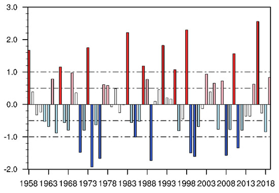
Figure 1.
Time series of normalized DJF Niño−3.4 index from 1958 to 2019. Dashed lines indicate 0.5 (−0.5) and 1.0 (−1.0) standard deviations, respectively. Light red (light blue) bars denote relatively weaker El Niño (La Niña) events and red (blue) bars denote relatively stronger El Niño (La Niña) events.

Table 1.
The selected strong and weak El Niño/La Niña events during 1958–2019.
Figure 2 shows the composite DJF SSTA for strong and weak El Niño/La Niña events, respectively. It is interesting to notice that a stronger El Niño shifts its maximum location eastward, approximately located around 120° W (Figure 2a), while a stronger La Niña tends to shift its SSTA center westward, approximately around 160° W (Figure 2c). In contrast, the SSTA center for a weaker El Niño lies more westward than stronger El Niño, which implies that the amplitude for El Niño that appears in central Pacific tends to be weaker (Figure 2b). Similarly, for La Niña events, the amplitude is weaker when its SSTA center is shown more to the east (Figure 2d). This raises a very interesting scientific question about the spatial structure asymmetry between El Niño and La Niña: why does a stronger El Niño favor developing towards the eastern Pacific while a stronger La Niña favors developing towards the central Pacific?
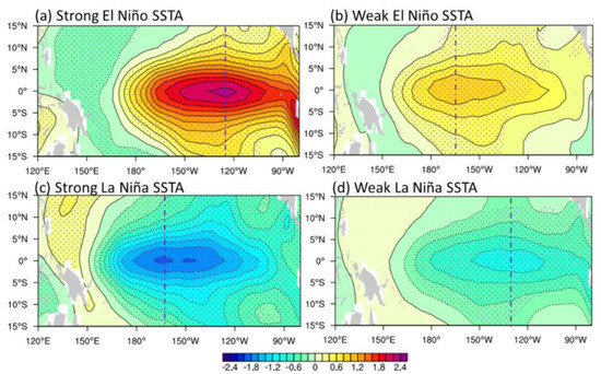
Figure 2.
Composite DJF SSTA (shading, °C) for strong and weak El Niño (a,b)/La Niña (c,d). The dotted region denotes above 90% confidence level.
3.2. Temperature Skewness
As we show in the previous subsection, the stronger El Niño (La Niña) tends to shift its center to the equatorial eastern (central) Pacific, which implies that the amplitude of stronger El Niño might be stronger (weaker) than La Niña in the eastern (central) Pacific. To verify the link between the spatial structure asymmetry and the amplitude asymmetry, the skewness of SSTA is further calculated (Figure 3a). It is interesting to note that positive skewness is presented in the equatorial eastern Pacific, while negative skewness is shown in the equatorial central Pacific, which indicates that the amplitude for El Niño events is stronger (weaker) than La Niña events in the equatorial eastern (central) Pacific. Therefore, the zonally asymmetric feature of ENSO spatial structure is closely linked to the longitudinal distribution of SSTA skewness along the equator. As the skewness measures the general features between El Niño and La Niña, we also calculated the asymmetric component of the composite SSTA for total El Niño and total La Niña events (Figure 3b). Here, the asymmetric component is defined as the sum of the composite El Niño and La Niña SSTA, following [45]. It was shown that the pattern of asymmetric component of SSTA between total El Niño and La Niña resembles the SSTA skewness to a large extent. In the following, we will analyze the physical cause of the spatial structure asymmetry of El Niño and La Niña based on a mixed-layer heat budget analysis. To reveal general nonlinear dynamical heating feature of ENSO, we will compose all El Niño and La Niña cases. As the positive (negative) skewness is mainly located to the east of 120° W (west of 170° W), the mixed-layer heat budget analysis will be conducted over the equatorial central Pacific (5° N–5° S, 160° E–170° W, red box in Figure 3) and the equatorial eastern Pacific (5° N–5° S, 120°–90° W, blue box in Figure 3).

Figure 3.
(a) DJF SSTA skewness; (b) asymmetric component of composite SSTA (shading, °C) for total El Niño and La Niña events. Red box denotes the central Pacific (5° N–5° S, 160° E–170° W) and blue box represents the eastern Pacific (5° N–5° S, 120°–90° W).
4. The Physical Causes of the Spatial Structure Asymmetry between El Niño and La Niña
In this section, the mixed-layer heat budget results will be shown to reveal the physical causes of the spatial structure asymmetry between El Niño and La Niña. As we examine the SSTA spatial structure during ENSO mature phase, the MLT budget is conducted towards ENSO developing phase (June-November). Figure 4 shows the MLT budget results for El Niño and La Niña over the equatorial central Pacific and the eastern Pacific. Note that an eastward extension of the diagnosis region in the equatorial eastern Pacific by 10° yields similar results. Although the MLT budget is not exactly in a balance due possibly to some subgrid processes and the uncertainties of ocean reanalysis data and heat flux data, the relative strength of the MLTA tendency terms (dT’⁄dt) calculated directly from the reanalysis data also show similarities to that calculated by Equation (1) (sum term) (Figure 4a,b), giving us the confidence to make further analyses. It was shown that over the central Pacific, the amplitude of the MLT tendency is stronger for La Niña than El Niño (Figure 4a), indicating that the negative SSTA development for La Niña is larger than the positive SSTA development for El Niño. In contrast, over the eastern Pacific, the positive MLT tendency for El Niño is stronger than its negative counterpart for La Niña (Figure 4b), which suggests a larger growth for El Niño events. Moreover, Figure 4 shows that the MLT tendency is mostly contributed by the dynamic terms, while the net surface heat flux terms tend to dampen the SSTA development for both El Niño and La Niña.
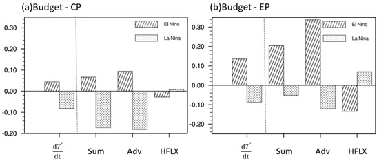
Figure 4.
The mixed−layer budget results over the (a) equatorial central Pacific (5° S–5° N, 160° E–170° W) and (b) the eastern Pacific (5° S–5° N, 120°–90° W). Along the x axis is the observed MLT tendency, the MLT tendency calculated by (Equation (1)), the three-dimensional total ocean temperature advection, the surface heat flux. Hatched bar and dotted bar represent composite results for El Niño and La Niña events, respectively.
In the following, we will focus on explaining the role of the dynamic terms in causing the asymmetry of MLT tendency for El Niño and La Niña events over the equatorial central and the eastern Pacific, respectively. For the dynamic terms (zonal/meridional/vertical ocean temperature advection), each term is further decomposed into two linear and one nonlinear term (see description of the linear and nonlinear terms in Section 2.2) following Su et al. [13]. Figure 5a,b shows the decomposition of temperature advection terms into linear and nonlinear terms for El Niño and La Niña events over the equatorial central Pacific (Figure 5a) and the eastern Pacific (Figure 5b). Note that over the equatorial central Pacific region (Figure 5a), the linear term for El Niño is positive and La Niña is negative, which favors the development of positive (negative) SSTA for El Niño (La Niña) events. However, the nonlinear terms are negative for both El Niño and La Niña, which tend to weaken the El Niño and strengthen the La Niña development in this particular region. It is interesting to note that although the linear terms for El Niño in the region are larger than those of La Niña, the total advection contribution for El Niño is smaller than that of La Niña due to the nonlinear advective effect (Figure 5a). This explains physically why the ocean dynamics over the equatorial central Pacific are more favorable for the growth of La Niña than El Niño. On the contrary, such an ocean dynamic role is very different over the equatorial eastern Pacific. Figure 5b shows that whereas the linear advection terms are positive for El Niño and negative for La Niña, which contributes to the growth of both El Niño and La Niña, the nonlinear advection terms are positive for both El Niño and La Niña. This implies that the nonlinear terms tend to enhance El Niño but weaken La Niña. While the sum of the linear terms for El Niño is comparable to that of La Niña, the total dynamic advection tendency for El Niño is almost three times as large as that of La Niña but due to the addition of the nonlinear terms (Figure 5b). This indicates that over the equatorial eastern Pacific, the ocean dynamics are more favorable for the growth of El Niño than La Niña.
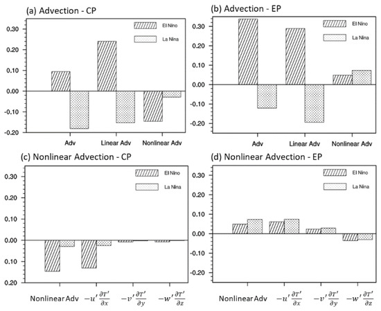
Figure 5.
The advection terms over the (a) equatorial central Pacific (5° S–5° N, 160° E–170° W) and the (b) eastern Pacific (5° S–5° N, 120°–90° W). Along the x axis is the total advection terms, linear advection terms and nonlinear advection terms. (c,d) Decomposition of nonlinear advection terms. Along the x axis is the total nonlinear advection, zonal nonlinear advection, meridional nonlinear advection and vertical nonlinear advection. Hatched bar and dotted bar represent composite results for El Niño and La Niña events, respectively.
Therefore, our budget analysis demonstrates that the nonlinear advection terms play important roles in shifting the ENSO center locations and causing asymmetric spatial structure between El Niño and La Niña. In the following, we further analyzed individual nonlinear advection terms in the equatorial central/eastern Pacific region, and the results are shown in Figure 5c,d. It was noted that in the equatorial central Pacific, nonlinear horizontal and vertical temperature advection terms are negative for both the El Niño and La Niña events, thus favoring a stronger La Niña and a weaker El Niño. Compared with the nonlinear horizontal advection, the nonlinear vertical advection plays a minor role over the central Pacific. In the eastern Pacific, the anomalous horizontal nonlinear temperature advection terms tend to be positive for both El Niño and La Niña, thus favoring a stronger growth of El Niño than La Niña. However, the nonlinear vertical temperature advection is negative for both, which tends to offset the nonlinear horizontal advection effect.
How does the nonlinear temperature advection affect the ENSO spatial structure asymmetry? To answer this question, we first examined the longitude-depth cross-section of the anomalous ocean temperature and ocean currents along the equatorial region (Figure 6a,b). For El Niño, the highest MLT anomaly is around 120° W and the zonal current anomaly in the mixed layer is eastward from central to the eastern Pacific (Figure 6a). According to Su et al. [13], zonal current anomaly is dominated by the geostrophic current in association with the thermocline depth variation. Therefore, the eastward current anomalies lead to a negative zonal nonlinear advection over the central Pacific (west of 170° W) while leading to a positive zonal nonlinear advection over the eastern Pacific (east of 120° W) (Figure 6a). Therefore, the zonal nonlinear advection tends to weaken El Niño in the central Pacific, while strengthening El Niño in the eastern Pacific. For the La Niña composite, the lowest MLT anomaly is also around 120° W. The anomalous westward current (u′ < 0) leads to a negative zonal nonlinear advection over the central Pacific (west of 170° W) while inducing positive zonal nonlinear advection over the eastern Pacific (east of 120° W) (Figure 6b). Therefore, La Niña tends to be strengthened in the central Pacific but weakened in the eastern Pacific due to the effect of nonlinear zonal advection.
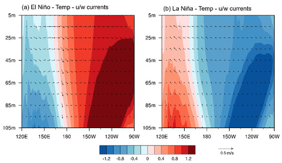
Figure 6.
Longitude−depth cross−section of the anomalous ocean temperature (shading; unit: °C) and zonal currents (vector; unit: m∙s−1)/vertical currents (vector; unit: 104 m∙s−1) along the equatorial region (within ±5°) at the development stage (June−November) of (a) El Niño and (b) La Niña.
Then, we analyzed the nonlinear meridional temperature advection via the longitudinal-depth cross-section of the ocean temperature and currents anomaly (Figure 7). It can be seen that for El Niño (La Niña), over the central Pacific, the maximum (minimum) MLT anomaly is located near the equator (Figure 7a,b) and the anomalous Ekman-induced meridional current is equatorward (poleward) in both hemispheres, causing negative nonlinear meridional advection for both El Niño and La Niña (Figure 7a,b). However, over the eastern Pacific, although the maximum (minimum) MLT anomaly for El Niño (La Niña) locates slightly south of the equator, the meridional current is northward (southward) (Figure 7c,d), which both generates positive meridional nonlinear advection (Figure 7c,d). According to Su et al. [13], over the eastern Pacific, due to the presence of climatological ITCZ (Inter-Tropical Convergence Zone) north of the equator, although the maximum (minimum) MLTA locates south of the equator, the anomalous convergence (divergence) appears north of the equator, which generates northward (southward) current for El Niño (La Niña). Therefore, the negative meridional nonlinear temperature advection tends to weaken (strengthen) El Niño (La Niña) in the central Pacific while the positive meridional nonlinear temperature advection tends to strengthen (weaken) El Niño (La Niña) in the eastern Pacific.
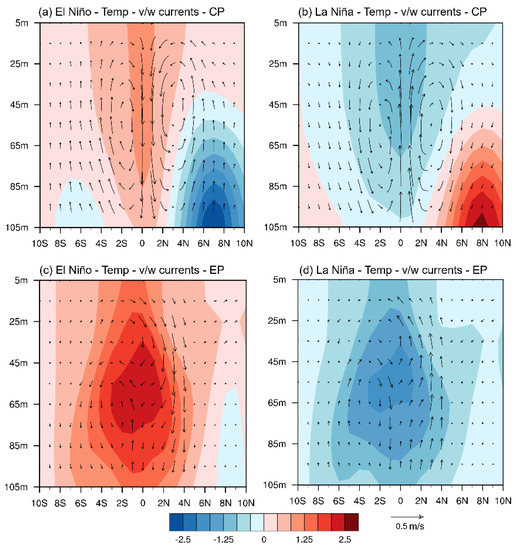
Figure 7.
Latitudinal−depth cross−section of the anomalous ocean temperature (shading; unit: °C) and meridional currents (vector; unit: m∙s−1)/vertical currents (vector; unit: 104 m∙s−1) averaged over the central Pacific (160° E–170° W) at the development stage (June–November) of (a) El Niño and (b) La Niña. (c,d) are the same as (a,b) but are averaged over the eastern Pacific (120°–90° W).
In addition, as the vertical temperature gradient is smaller in the mixed layer over the central Pacific (Figure 7a,b), the nonlinear vertical advection is small and plays a minor role. Over the eastern Pacific, the equatorial region (5° S–5° N) is dominated by anomalous downwelling (upwelling) for El Niño (La Niña) due to the convergence (divergence) of eastward (westward) geostrophic current [13]. This downwelling (upwelling) generates negative nonlinear vertical advection given the negative (positive) vertical temperature gradient (Figure 7c,d), acting to offset the nonlinear horizontal advection effects.
Therefore, it was found that nonlinear horizontal temperature advection, namely the nonlinear zonal and meridional advection are mainly responsible for the spatial structure asymmetry between El Niño and La Niña. Over the equatorial central Pacific, zonal and meridional nonlinear temperature advection terms tend to be negative for both the El Niño and La Niña events, thus favoring the development of a stronger La Niña and a weaker El Niño. Towards the eastern Pacific, the nonlinear horizontal temperature advection terms tend to be positive for both El Niño and La Niña, thus favoring a stronger growth for El Niño than La Niña. Anomalous nonlinear vertical temperature advection plays a minor role in the central Pacific and tends to offset the nonlinear horizontal advection effect in the equatorial eastern Pacific.
5. Conclusions and Discussions
In this study, the structure asymmetry between strong and weak El Niño and La Niña episodes is revealed via observational analyses. By decomposing El Niño and La Niña events into a strong group and a weak group, it was found that the strong El Niño group tends to shift its peak SSTA center towards the east relative to the weak El Niño group, whereas the strong La Niña group tends to shift its center towards the west compared to the weak La Niña group. This zonally asymmetric feature of ENSO spatial structure is closely linked to the longitudinal distribution of SSTA skewness along the equator. Positive SSTA skewness appears in the equatorial eastern Pacific, while negative skewness is located in the equatorial central Pacific, implying that the amplitude of El Niño events is stronger (weaker) than La Niña events in the equatorial eastern (central) Pacific. The skewness distribution is consistent with the ENSO structure asymmetry characteristic.
A further diagnosis of the ocean mixed-layer heat budget for El Niño and La Niña events demonstrates the importance of the nonlinear dynamic heating in contributing to the aforementioned ENSO pattern asymmetry. Although the linear terms contribute to the growth of both El Niño and La Niña in the equatorial central and the eastern Pacific, the nonlinear dynamic terms tend to be negative (positive) for both the El Niño and La Niña events in equatorial central (eastern) Pacific (Figure 8), causing a stronger growth of La Niña (El Niño) over the equatorial central (eastern) Pacific.
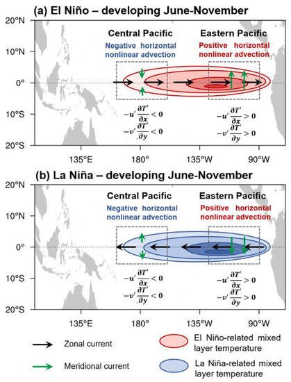
Figure 8.
Schematic diagram of nonlinear horizontal advection in causing spatial structure asymmetry for El Niño (a) and La Niña (b). Black/Green vectors indicate anomalous zonal/meridional currents; red/blue shading represents the El Niño−related/La Niña−related mixed−layer temperature anomaly during ENSO developing June–November).
The cause of the distinctive nonlinear temperature advection processes for El Niño and La Niña is further investigated and shown in a schematic diagram (Figure 8). Over the central Pacific, the westward (eastward) zonal currents for La Niña (El Niño) cause anomalous negative nonlinear zonal advection for both El Niño and La Niña. Meanwhile, the meridional current anomalies in CP are equatorward for El Niño and poleward for La Niña (Figure 8), which leads to a negative meridional nonlinear advection for both El Niño and La Niña (Figure 8). Over the equatorial eastern Pacific, as the maximum SSTA center is located near 120° W, the westward (eastward) zonal currents for La Niña (El Niño) cause anomalous positive nonlinear zonal advection for both El Niño and La Niña. Meanwhile, as the SSTA center associated with ENSO is located slightly south of the equator, the anomalous northward (southward) meridional current during El Niño (La Niña) (Figure 8) causes a positive nonlinear meridional temperature advection anomaly for both El Niño and La Niña (Figure 7c,d and Figure 8a,b).
To sum up, the mixed-layer budget analysis results indicate that the nonlinear horizontal temperature advection terms play an important role in causing the distinctive ENSO pattern asymmetry shown in Figure 2. Some previous studies [12,29] suggested a “thermocline outcropping” mechanism. The key premise behind this mechanism is the impact of the mean state on the anomalous wind stress–thermocline depth relationship. Because the mean ocean thermocline depth is shallow in the equatorial eastern Pacific, a nonlinear relation between anomalous wind stress in the central Pacific and anomalous thermocline anomaly in the eastern Pacific was assumed, that is, a westerly wind stress anomaly in the central Pacific could lead to a positive thermocline depth anomaly in the eastern Pacific, but an easterly wind stress anomaly in the central Pacific could not cause a comparable negative thermocline depth anomaly in situ because the thermocline might outcrop to the surface. An opposite argument was applied to the warm ocean such as the central Pacific or Indian Ocean where the mean thermocline is deep. In an Indian Ocean Dipole (IOD)-related work, it was demonstrated that such an argument is faulted [46]. Our further analysis (figure not shown) shows a linear relationship between the zonal wind stress anomaly in the central Pacific and the thermocline depth anomaly in the eastern Pacific (with a linear correlation coefficient of 0.9). There is no obvious asymmetry between positive and negative events, and the thermocline depth anomaly associated with La Niña can reach a similar amplitude as El Niño. Based on these results, we argue that the background mean SST/thermocline depth distribution does not play a critical role in causing the El Niño and La Niña pattern asymmetry discovered in the current study.
Moreover, given the observed characteristic shown in Figure 2, it is natural to ask what is the capability of the current state-of-art coupled atmosphere–ocean models in reproducing the ENSO pattern asymmetry feature. Therefore, a further diagnosis of the coupled model (such as CMIP6) simulations is needed. In addition to revealing the asymmetric spatial SSTA patterns, the diagnosis of the model’s nonlinear dynamical heating processes is also needed. Such diagnosis works will be performed in future endeavors.
Author Contributions
J.Y., T.L. and L.J. conceived the idea. J.Y. conducted the data analyses and prepared figures. All contribute in writing and revising the manuscript. All authors have read and agreed to the published version of the manuscript.
Funding
This research was supported by National Natural Science Foundation of China (NSFC), grant 42088101.
Institutional Review Board Statement
Not applicable.
Informed Consent Statement
Not applicable.
Data Availability Statement
The reanalysis datasets used in this study are available through the following websites: SODA224 at https://iridl.ldeo.columbia.edu/SOURCES/.CARTON-GIESE/.SODA/.v2p2p4/datasetdatafiles.html accessed on 11 November 2021; GODAS at https://cfs.ncep.noaa.gov/cfs/godas/monthly/ accessed on 11 November 2021; ORAS5 at https://icdc.cen.uni-hamburg.de/thredds/catalog/ftpthredds/EASYInit/oras5/r1x1/catalog.html and https://icdc.cen.uni-hamburg.de/thredds/catalog/ftpthredds/EASYInit/oras5_backward_extension/r1x1/catalog.html accessed on 9 November 2022; NCEP at https://psl.noaa.gov/data/gridded/data.ncep.reanalysis2.html accessed on 11 November 2021; 20CRv2 at https://psl.noaa.gov/data/gridded/data.20thC_ReanV2.html accessed on 22 August 2022; ERA5 at https://cds.climate.copernicus.eu/#!/search?text=ERA5&type=dataset on 25 November 2021.
Acknowledgments
We thank three anonymous reviewers for their valuable comments and work was supported by NSFC grant 42088101.
Conflicts of Interest
The authors declare no conflict of interest.
References
- Horel, J.D.; Wallace, J.M. Planetary-Scale Atmospheric Phenomena Associated with the Southern Oscillation. Mon. Weather Rev. 1981, 109, 813–829. [Google Scholar] [CrossRef]
- Philander, S.G.H. El Niño Southern Oscillation Phenomena. Nature 1983, 302, 295–301. [Google Scholar] [CrossRef]
- Ropelewski, C.F.; Halpert, M.S. Global and Regional Scale Precipitation Patterns Associated with the El Niño/Southern Oscillation. Mon. Weather Rev. 1987, 115, 1606–1626. [Google Scholar] [CrossRef]
- McPhaden, M.J.; Zebiak, S.E.; Glantz, M.H. ENSO as an Integrating Concept in Earth Science. Science 2006, 314, 1740–1745. [Google Scholar] [CrossRef]
- Li, T.; Hsu, P. Dynamics of El Niño–Southern Oscillation. In Fundamentals of Tropical Climate Dynamics; Springer Atmospheric Sciences; Springer International Publishing: Cham, Switzerland, 2018; pp. 149–183. ISBN 978-3-319-59595-5. [Google Scholar]
- Capotondi, A.; Wittenberg, A.T.; Newman, M.; Di Lorenzo, E.; Yu, J.-Y.; Braconnot, P.; Cole, J.; Dewitte, B.; Giese, B.; Guilyardi, E.; et al. Understanding ENSO Diversity. Bull. Am. Meteorol. Soc. 2015, 96, 921–938. [Google Scholar] [CrossRef]
- Timmermann, A.; An, S.-I.; Kug, J.-S.; Jin, F.-F.; Cai, W.; Capotondi, A.; Cobb, K.M.; Lengaigne, M.; McPhaden, M.J.; Stuecker, M.F.; et al. El Niño–Southern Oscillation Complexity. Nature 2018, 559, 535–545. [Google Scholar] [CrossRef] [PubMed]
- Wang, B.; Luo, X.; Yang, Y.-M.; Sun, W.; Cane, M.A.; Cai, W.; Yeh, S.-W.; Liu, J. Historical Change of El Niño Properties Sheds Light on Future Changes of Extreme El Niño. Proc. Natl. Acad. Sci. USA 2019, 116, 22512–22517. [Google Scholar] [CrossRef]
- Hoerling, M.P.; Kumar, A.; Zhong, M. El Niño, La Niña, and the Nonlinearity of Their Teleconnections. J Clim. 1997, 10, 1769–1786. [Google Scholar] [CrossRef]
- Frauen, C.; Dommenget, D.; Tyrrell, N.; Rezny, M.; Wales, S. Analysis of the Nonlinearity of El Niño–Southern Oscillation Teleconnections. J. Clim. 2014, 27, 6225–6244. [Google Scholar] [CrossRef]
- Hannachi, A.; Stephenson, D.B.; Sperber, K.R. Probability-Based Methods for Quantifying Nonlinearity in the ENSO. Clim. Dyn. 2004, 22, 69–70. [Google Scholar] [CrossRef]
- An, S.-I.; Jin, F.-F. Nonlinearity and Asymmetry of ENSO. J. Clim. 2004, 17, 2399–2412. [Google Scholar] [CrossRef]
- Su, J.; Zhang, R.; Li, T.; Rong, X.; Kug, J.-S.; Hong, C.-C. Causes of the El Niño and La Niña Amplitude Asymmetry in the Equatorial Eastern Pacific. J. Clim. 2010, 23, 605–617. [Google Scholar] [CrossRef]
- Frauen, C.; Dommenget, D. El Niño and La Niña Amplitude Asymmetry Caused by Atmospheric Feedbacks: Atmospheric Causes for Enso Asymmetry. Geophys. Res. Lett. 2010, 37, L18801. [Google Scholar] [CrossRef]
- Kessler, W.S. Is ENSO a Cycle or a Series of Events? Geophys. Res. Lett. 2002, 29, 40-1–40-44. [Google Scholar] [CrossRef]
- Larkin, N.K.; Harrison, D.E. ENSO Warm (El Niño) and Cold (La Niña) Event Life Cycles: Ocean Surface Anomaly Patterns, Their Symmetries, Asymmetries, and Implications. J. Clim. 2002, 15, 1118–1140. [Google Scholar] [CrossRef]
- McPhaden, M.J.; Zhang, X. Asymmetry in Zonal Phase Propagation of ENSO Sea Surface Temperature Anomalies. Geophys. Res. Lett. 2009, 36, L13703. [Google Scholar] [CrossRef]
- Okumura, Y.M.; Deser, C. Asymmetry in the Duration of El Niño and La Niña. J. Clim. 2010, 23, 5826–5843. [Google Scholar] [CrossRef]
- Chen, M.; Li, T.; Shen, X.; Wu, B. Relative Roles of Dynamic and Thermodynamic Processes in Causing Evolution Asymmetry between El Niño and La Niña. J. Clim. 2016, 29, 2201–2220. [Google Scholar] [CrossRef]
- Wu, X.; Okumura, Y.M.; DiNezio, P.N. What Controls the Duration of El Niño and La Niña Events? J. Clim. 2019, 32, 5941–5965. [Google Scholar] [CrossRef]
- Ashok, K.; Behera, S.K.; Rao, S.A.; Weng, H.; Yamagata, T. El Niño Modoki and Its Possible Teleconnection. J. Geophys. Res. 2007, 112, C11007. [Google Scholar] [CrossRef]
- Kao, H.-Y.; Yu, J.-Y. Contrasting Eastern-Pacific and Central-Pacific Types of ENSO. J. Clim. 2009, 22, 615–632. [Google Scholar] [CrossRef]
- Kug, J.-S.; Jin, F.-F.; An, S.-I. Two Types of El Niño Events: Cold Tongue El Niño and Warm Pool El Niño. J. Clim. 2009, 22, 1499–1515. [Google Scholar] [CrossRef]
- Schopf, P.S.; Burgman, R.J. A Simple Mechanism for ENSO Residuals and Asymmetry. J. Clim. 2006, 19, 3167–3179. [Google Scholar] [CrossRef]
- Capotondi, A.; Wittenberg, A.T.; Kug, J.; Takahashi, K.; McPhaden, M.J. ENSO Diversity. In Geophysical Monograph Series; McPhaden, M.J., Santoso, A., Cai, W., Eds.; Wiley: Hoboken, NJ, USA, 2020; pp. 65–86. ISBN 978-1-119-54816-4. [Google Scholar]
- Kug, J.-S.; Ham, Y.-G. Are There Two Types of La Nina?: Two Types of la Nina. Geophys. Res. Lett. 2011, 38, L16704. [Google Scholar] [CrossRef]
- Takahashi, K.; Dewitte, B. Strong and Moderate Nonlinear El Niño Regimes. Clim. Dyn. 2016, 46, 1627–1645. [Google Scholar] [CrossRef]
- Battisti, D.S.; Hirst, A.C. Interannual Variability in a Tropical Atmosphere–Ocean Model: Influence of the Basic State, Ocean Geometry and Nonlinearity. J. Atmospheric Sci. 1989, 46, 1687–1712. [Google Scholar] [CrossRef]
- Galanti, E.; Tziperman, E.; Harrison, M.; Rosati, A.; Giering, R.; Sirkes, Z. The Equatorial Thermocline Outcropping—A Seasonal Control on the Tropical Pacific Ocean–Atmosphere Instability Strength. J. Clim. 2002, 15, 2721–2739. [Google Scholar] [CrossRef]
- Yu, J.-Y.; Liu, W.T. A Linear Relationship between ENSO Intensity and Tropical Instability Wave Activity in the Eastern Pacific Ocean: Relationship between Enso and Tiws. Geophys. Res. Lett. 2003, 30, 1735. [Google Scholar] [CrossRef]
- An, S.-I. Interannual Variations of the Tropical Ocean Instability Wave and ENSO. J. Clim. 2008, 21, 3680–3686. [Google Scholar] [CrossRef]
- Timmermann, A. A Nonlinear Mechanism for Decadal El NiñO Amplitude Changes. Geophys. Res. Lett. 2002, 29, 1003. [Google Scholar] [CrossRef]
- Huang, B.; Thorne, P.W.; Banzon, V.F.; Boyer, T.; Chepurin, G.; Lawrimore, J.H.; Menne, M.J.; Smith, T.M.; Vose, R.S.; Zhang, H.-M. Extended Reconstructed Sea Surface Temperature, Version 5 (ERSSTv5): Upgrades, Validations, and Intercomparisons. J. Clim. 2017, 30, 8179–8205. [Google Scholar] [CrossRef]
- Carton, J.A.; Giese, B.S. A Reanalysis of Ocean Climate Using Simple Ocean Data Assimilation (SODA). Mon. Weather Rev. 2008, 136, 2999–3017. [Google Scholar] [CrossRef]
- Behringer, D.W. The Global Ocean Data Assimilation System (GODAS) at NCEP. In Proceedings of the 11th symposium on integrated observing and assimilation systems for the atmosphere, oceans, and land surface, San Antonio, TX, USA, 14–18 January 2007. [Google Scholar]
- Zuo, H.; Balmaseda, M.A.; Mogensen, K.; Tietsche, S. OCEAN5: The ECMWF Ocean Reanalysis System and its Real-Time Analysis Component; European Centre for Medium-Range Weather Forecasts: Reading, UK, 2018; p. 44. [Google Scholar]
- Compo, G.P.; Whitaker, J.S.; Sardeshmukh, P.D.; Matsui, N.; Allan, R.J.; Yin, X.; Gleason, B.E.; Vose, R.S.; Rutledge, G.; Bessemoulin, P.; et al. The Twentieth Century Reanalysis Project: The Twentieth Century Reanalysis Project. Q. J. R. Meteorol. Soc. 2011, 137, 1–28. [Google Scholar] [CrossRef]
- Kanamitsu, M.; Ebisuzaki, W.; Woollen, J.; Yang, S.-K.; Hnilo, J.J.; Fiorino, M.; Potter, G.L. NCEP–DOE AMIP-II Reanalysis (R-2). Bull. Am. Meteorol. Soc. 2002, 83, 1631–1644. [Google Scholar] [CrossRef]
- Hersbach, H.; Bell, B.; Berrisford, P.; Hirahara, S.; Horányi, A.; Muñoz-Sabater, J.; Nicolas, J.; Peubey, C.; Radu, R.; Schepers, D.; et al. The ERA5 Global Reanalysis. Q. J. R. Meteorol. Soc. 2020, 146, 1999–2049. [Google Scholar] [CrossRef]
- White, G.H. Skewness, kurtosis and extreme values of northern hemisphere geopotential heights. Mon. Weather. Rev. 1980, 108, 1446–1455. [Google Scholar] [CrossRef]
- Li, T.; Zhang, Y.; Lu, E.; Wang, D. Relative Role of Dynamic and Thermodynamic Processes in the Development of the Indian Ocean Dipole: An OGCM Diagnosis: Dynamic and thermodynamic processes. Geophys. Res. Lett. 2002, 29, 25-1–25-4. [Google Scholar] [CrossRef]
- Chen, L.; Li, T.; Yu, Y. Causes of Strengthening and Weakening of ENSO Amplitude under Global Warming in Four CMIP5 Models. J. Clim. 2015, 28, 3250–3274. [Google Scholar] [CrossRef]
- Chen, L.; Li, T.; Yu, Y.; Behera, S.K. A Possible Explanation for the Divergent Projection of ENSO Amplitude Change under Global Warming. Clim. Dyn. 2017, 49, 3799–3811. [Google Scholar] [CrossRef]
- Pan, X.; Li, T.; Chen, M. Change of El Niño and La Niña Amplitude Asymmetry around 1980. Clim. Dyn. 2020, 54, 1351–1366. [Google Scholar] [CrossRef]
- Wu, B.; Li, T.; Zhou, T. Asymmetry of Atmospheric Circulation Anomalies over the Western North Pacific between El Niño and La Niña. J. Clim. 2010, 23, 4807–4822. [Google Scholar] [CrossRef]
- Hong, C.-C.; Li, T. The independence of SST skewness to thermocline feedback in the eastern equatorial Indian Ocean. Geophys. Res. Lett. 2010, 37, L11702. [Google Scholar] [CrossRef]


Disclaimer/Publisher’s Note: The statements, opinions and data contained in all publications are solely those of the individual author(s) and contributor(s) and not of MDPI and/or the editor(s). MDPI and/or the editor(s) disclaim responsibility for any injury to people or property resulting from any ideas, methods, instructions or products referred to in the content. |
© 2023 by the authors. Licensee MDPI, Basel, Switzerland. This article is an open access article distributed under the terms and conditions of the Creative Commons Attribution (CC BY) license (https://creativecommons.org/licenses/by/4.0/).