Sichuan Rainfall Prediction Using an Analog Ensemble

Abstract

This study aimed to address the significant bias in 0–44-day precipitation forecasts under numerical weather conditions. To achieve this, we utilized observational data obtained from 156 surface stations in the Sichuan region and reanalysis grid data from the National Centers for Environmental Prediction Climate Forecast System Model version 2. Statistical analysis of the spatiotemporal characteristics of precipitation in Sichuan was conducted, followed by a correction experiment based on the Analog Ensemble algorithm for 0–44-day precipitation forecasts for different seasons in the Sichuan region. The results show that, in terms of spatial distribution, the precipitation amounts and precipitation days in Sichuan Province gradually decreased from east to west. Temporally, the highest number of precipitation days occurred in autumn, while the maximum precipitation amount was observed in summer. The Analog Ensemble algorithm effectively reduced the error in the model forecast results for different seasons in the Sichuan region. However, the correction effectiveness varied seasonally, primarily because of the differing performance of the AnEn method in relation to precipitation events of various magnitudes. Notably, the correction effect was the poorest for heavy-rain forecasts. In addition, the degree of improvement of the Analog Ensemble algorithm varied for different initial forecast times and forecast lead times. As the forecast lead time increased, the correction effect gradually weakened.

1. Introduction

The Sichuan Basin (SCB) in southwestern China is situated on the Tibetan Plateau, Yunnan–Guizhou Plateau, Wu Mountains, and Daba Mountains. Due to its unique topography, the SCB region is at risk of frequent heavy rainfall events during the warm season, resulting in severe floods and landslides that cause significant damage to life and property [1]. As a result of advancements in supercomputing and numerical weather prediction (NWP) methodologies, NWP can deliver continuous heavy-rainfall forecasts ranging from minutes to months [2,3,4]. Nevertheless, the capacity of NWP to forecast heavy precipitation in the SCB region is constrained, particularly in the context of large-scale precipitation prediction, because of its complex topographic characteristics [5,6,7,8]. Previous studies have shown that precipitation patterns in complex mountainous terrains are influenced by a variety of topographic factors and that the spatial representativeness of precipitation station observation data is poor, limiting the applicability and accuracy of remote sensing, reanalysis of meteorological products, and traditional interpolation methods [9]. Moreover, research has indicated that because of terrain complexity, sparse distribution of ground precipitation observation stations in remote areas, the limited number and maintenance difficulties of observation stations in high-altitude areas, and the accompanying three-dimensional climate in complex terrain regions, existing station data face challenges in providing accurate spatiotemporal precipitation-distribution information [10]. The external forcing of special terrain and the limited forecasting capabilities of global numerical prediction models and high-resolution mesoscale numerical models lead to difficulties in predicting heavy rainfall in mountainous areas [11].

To reduce the systematic and random errors of NWP in complex terrain, previous studies have explored statistical and machine learning methods and made corrections to model output results [12]. Research has been conducted on the correction of precipitation forecasts. For instance, Luca et al. [13] employed the weighted average of simulated observations for post-processing numerical weather forecasts, achieving a 35% improvement compared to the original predictions. Falck et al. [14] investigated the use of stochastic error models with empirical rainfall ensemble datasets, which improved the regional numerical weather forecast model by 60%. Zhao et al. [15] implemented a combination of nonlinear and nonparametric algorithms to optimize numerical weather forecast data, correcting probability density values and adjusting errors, leading to the effective integration of physical and statistical information and improved forecast accuracy. De Giorgi et al. [12] utilized numerical weather parameters that had the greatest impact on improved statistical models for post-processing numerical weather forecast results, effectively increasing the forecasting ability for power generation in complex-region wind farms. Nandar et al. [16] designed a weather forecasting system based on the Bayesian Network (BN) model, which displayed conditional probabilities and causal relationships between variables, achieving acceptable forecast accuracy in experimental results. Zhao et al. [17] proposed an innovative method for correcting precipitation forecasts of the European Centre for Medium-Range Weather Forecasts (ECMWF) by combining convolutional neural networks (CNN) and random forest regression models. In this method, the classification of station precipitation-forecast values according to the ECMWF model was first conducted, followed by the calculation of high-correlation factor matrices corresponding to different levels.

The Analog Ensemble (AnEn) technique serves as a significant method for forecast correction [18]. Monache et al. [18] introduced an analog-based strategy known as the analog ensemble (AnEn). To create ensembles, this method estimates the probability distribution of future atmospheric conditions by using a collection of historical observations that best resemble a deterministic NWP. AnEn has been demonstrated to be effective in various meteorological applications, such as probabilistic precipitation forecasts, 850 hPa temperature, 2 m temperature, and 10 m wind speed [13,19,20,21] Cervone et al. [22] employed artificial neural networks (ANN) and AnEn to correct synthetic data generated by 4450 solar power plants, constructing deterministic probability forecasts for the next 72 h. Hu et al. [23] proposed an evolutionary algorithm for dynamically and automatically learning optimal unstructured grid patterns to reduce spatial and temporal inconsistencies in some physical changes. The results demonstrate that the algorithm can optimize the available computational resources and generate probabilistic forecasts in the AnEn model. Junk et al. [24] designed static and dynamic weighting algorithms to enhance the effectiveness of AnEn in wind power forecasting; the results showed a 20% improvement over the original predictions for both onshore and offshore sites. Monache et al. [18] applied the AnEn method to precipitation forecasting, providing an excellent solution for assessing the uncertainty of precipitation forecasts.

The aim of this study was to address the significant biases present in 0–44-day precipitation forecasts in numerical weather prediction by utilizing observation data from 156 surface stations in Sichuan Province and reanalysis grid data from the National Centers for Environmental Prediction Coupled Forecast System Model version 2 (NCEP CFSv2). The AnEn algorithm was implemented in experimental settings to correct 0–44-day precipitation forecasts across various seasons in Sichuan Province. These experiments analyzed the numerical prediction errors in extended-range precipitation forecasts and investigated appropriate methods for adjusting these forecasts in the region, utilizing CFSv2 precipitation forecasts (beginning at 00 UTC) from 1 January 2017, to 30 December 2020. The goal of this study was to contribute to the development of effective strategies for mitigating the risks associated with natural disasters in Sichuan Province. The remainder of this article is structured as follows: Section 2 offers a comprehensive overview of the data and methods employed in this study; Section 3 presents a statistical analysis of the spatiotemporal characteristics of precipitation in Sichuan; Section 4 examines the comparison results between the CFSv2 model and observed values, along with the implications of bias correction; finally, Section 5 provides a summary and in-depth discussion of the research findings.

2. Overview of the Study Area

Sichuan Province is located in western China. Owing to its geographical position at the intersection of the first and second steps of China’s topographical gradient, Sichuan Province exhibits diverse and complex terrain characteristics with significant fluctuations in landforms and considerable differences in elevation (Figure 1). The western region of Sichuan is dominated by plateau topography, with higher elevations towards the west, making it part of the Qinghai–Tibet Plateau and the Transverse Mountain Range. Moving eastward from the western region, the terrain descends rapidly and enters the lowest elevation area of the second step, the Sichuan Basin. Compared to the western region, the basin has a relatively flat terrain and lower elevation, with a dense distribution of meteorological stations. Numerical prediction models encounter challenges in handling steep, tall, and complex terrains such as plateaus, mountains, and plains, along with their associated physical processes. Moreover, the scarcity and sparse distribution of meteorological observation data in these complex regions further complicate precipitation forecasting.

3. Data and Methodology

3.1. Data and Pre-Processing

In this study, daily precipitation observation data from 156 national meteorological stations in Sichuan Province, China, were collected from 2017 to 2020. The data were sourced from the Sichuan Climate Center. The distribution of these stations is shown in Figure 1. The topography of the Sichuan region is complex, with diverse geographical features such as plateaus, mountains, and hills. Plains areas have a higher density of meteorological stations than complex terrain regions, and the border areas between the plateau and mountainous regions exhibit a concentrated distribution of stations, such as those in Chengdu (red triangle in Figure 1). The northwestern mountainous area has a high elevation and sparse, uneven distribution of meteorological stations, whereas the eastern plains of Sichuan have a relatively flat topography and a uniform distribution of stations.

Subsequently, daily precipitation data from the meteorological stations were processed as a preparatory step for model correction. To maintain data continuity and adhere to the longest time principle, this study implemented three quality control methods, namely, internal consistency check, climatic boundary value check, and station extreme value check, while interpolating missing data using moving-average and anomaly-detection methods and smoothing daily precipitation data to mitigate the impact of short-term fluctuations on the analysis [25].

We also screened for missing data; if a station had more than 5% of the data missing in a year, that year’s data for the station were considered missing and only stations without missing data were retained. For stations with relocation issues, the criteria established by Zhai and Ren [26] were used: if a station’s location moved more than 20 km or its elevation changed by more than 50 m, the station was excluded.

Daily ground precipitation forecasts for the 44-day future period from 2017 to 2020 were obtained using the CFSv2 model. Numerical forecast grid data were derived from the NCEP CFSv2. The NCEP-CFSv2 model is a real-time dynamic prediction system developed by the U.S. Environmental Prediction Center that comprehensively considers the impacts of the oceans, land, sea ice, and atmosphere. The model data include hindcasts from 1982 to 2019 and real-time forecasts. Each month, the model integrates the initial fields for four different times, with 24–28 ensemble members for prediction at a resolution of 1° latitude × 1° longitude. CFSv2 is an upgraded version of CFSv1 with an improved data assimilation system, for land, ocean, and initial conditions. The atmospheric component uses the NCEP Global Forecast Model, the ocean component uses the GFDL MOM4 model, and the land component uses a 4-layer land surface model. The initial fields were based on National Center for Environmental Prediction (NCEP) Climate Forecast System Reanalysis (CFSR) [27].

The precipitation forecast for Sichuan Province was obtained through a bilinear interpolation process, which was used to interpolate CFSv2 data to 156 specific locations within the province. The study area was systematically divided into regular grids, with each grid point serving as a reference node for interpolation. The four nearest CFSv2 data points were identified for each of the 156 target locations, based on their proximity.

A bilinear interpolation method was employed to estimate the precipitation at a specific target location. This method uses a weighted average of the four nearest data points. The interpolation weights were computed by considering the distances between the target location and surrounding CFSv2 data points. The closer a data point to the target location, the higher the weight assigned during the interpolation process. By applying these calculated weights, the CFSv2 precipitation values were interpolated for each of the 156 target locations within the province.

3.2. Method

3.2.1. AnEn Method

Monache et al. [18] introduced the AnEn method to derive uncertainty forecasts from deterministic forecasts. This approach calculates uncertainty information using a set of M historical verifying observations (e.g., wind power) associated with M historical forecasts (analogs) that closely resemble current deterministic forecasts. By directly incorporating the verified observations as ensemble members, any observational errors in the verification were instantly accounted for. A cost function was employed to determine the multivariate metric that measured the similarity between the present deterministic forecast and past predictions from a historical dataset [28,29,30,31,32].

$$\left|\left|F_t,A_{t^{\mathrm{\prime }}}\right|\right|=\sum _{i=1}^{N_v}\frac{w_i}{{\sigma }_{f_i}}\sqrt{\sum _{j=-\tilde{t}}^{\tilde{t}}{\left(F_{i,t+j}-A_{{i,t}^{\mathrm{\prime }}+j}\right)}^2}$$

(1)

At the same spatial location, $F_t$ denotes the model forecast for the future at current time t; $A_t$ refers to the historical forecast at a similar initial time and forecast lead time in the current deterministic forecast; $N_v$ and $w_i$ represent the number of forecast factors associated with the forecast element and their respective weights (in this study, $N_v$ is set to 1, making $w_i$ equal to 1) [33,34,35,36]; ${\sigma }_{f_i}$ signifies the standard deviation of the historical time series for the ith factor; and $\tilde{t}$ corresponds to the time window (in this study, $\tilde{t}$ is set to 1, meaning both the previous and subsequent time steps of the current forecast are considered for calculation). $\left|\left|F_t,A_{t^{\mathrm{\prime }}}\right|\right|$ can be interpreted as the ‘distance’ between the two factors in a multidimensional vector space, with a smaller ‘distance’ indicating a higher similarity between them [37,38].

3.2.2. Evaluation Method

The Root-Mean-Square Error (RMSE) was obtained by computing the squared differences between the predicted and observed values, calculating their average, and taking the square root of the average. A lower RMSE typically indicates a better fit between the predictions and actual observations [39].

$$E_{RMSE}={\left[\frac{1}{n}{\sum }_{i=1}^n {\left(f_i-o_i\right)}^2\right]}^{\frac{1}{2}}$$

(2)

where n is the number of lattice samples in the space field, $f_i$ is the forecast value of the ith sample, and $o_i$ is the observation of the ith sample [40]. RMSE quantifies the discrepancy between the forecasted and analyzed fields; a larger value indicates a greater forecasting error [41].

3.2.3. Interpolation Methods: Bilinear Interpolation

To acquire extensive spatial precipitation data, this study employed a bilinear interpolation approach to interpolate the grid data to the corresponding observation stations, as described by Li and Heap [42,43]. The interpolation process also handled missing or irregular daily precipitation data based on spatial autocorrelation.

First, we collected the grid and station data and established the interpolation range. Subsequently, at each time step, an individual bilinear interpolation was performed for each station. For each target station, the four nearest grid points were identified and a weighted average was calculated using the data from these grid points and their relative distances to the target station, ultimately deriving the estimated value for the target station. This process was iterated throughout the entire time range until the daily precipitation data from all stations displayed comprehensive spatial distribution information. Utilizing this method, the study accomplished the cyclical interpolation of multiyear grid data, setting the groundwork for subsequent correction efforts [44,45,46].

We estimated the value at point (x,y) on a rectangular grid; the coordinates and values of the four corners of the rectangle were ($x_1$, $y_1$, $f_1$), ($x_1$, $y_2$, $f_2$), ($x_2{,y}_1$, $f_3$), and ($x_2$, $y_2$, $f_4$), where $x_1$< x < $x_2$ and $y_1$< y < $y_2$. The estimated value of f(x,y) at point (x,y) is:

$$\begin{gathered} f(x,y)=\frac{1}{(x_2-x_1)(y_2-y_1)}[f_1(x_2-x)(y_2-y)+f_3(x-x_1)(y_2-y)+f_2(x_2- \\ x)(y-y_1)+f_4(x-x_1)(y-y_1)] \end{gathered}$$

(3)

where (x,y) are the coordinates of the point to be estimated, f(x,y) is the estimated value, $f_1$, $f_2$, $f_3$, and $f_4$ are the values at the four corners of the rectangle, and $x_1$,$y_1$, $x_2$, and $y_2$ are the coordinates of the four corners of the rectangle [47,48,49].

4. Statistical Characteristics of Surface Precipitation Observations and Forecasts

To improve the accuracy of rainfall prediction models, it is imperative to conduct a statistical analysis of precipitation characteristics across different regions in Sichuan. Furthermore, comparative assessments of the model prediction errors for different seasons are required. The key parameters required for the corrections in this study were derived from statistical analyses.

4.1. Spatial Distribution Characteristics of Annual Precipitation in Sichuan

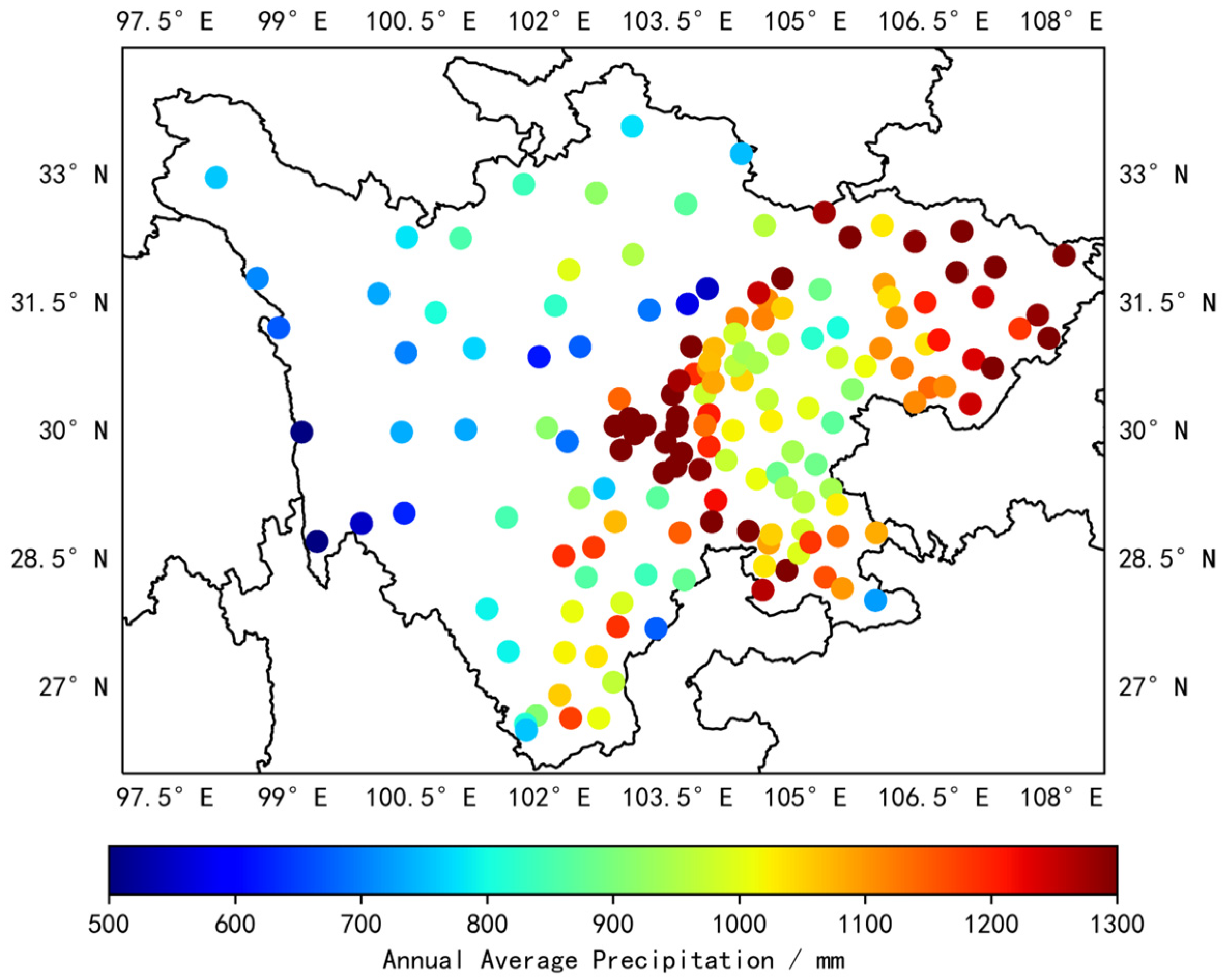
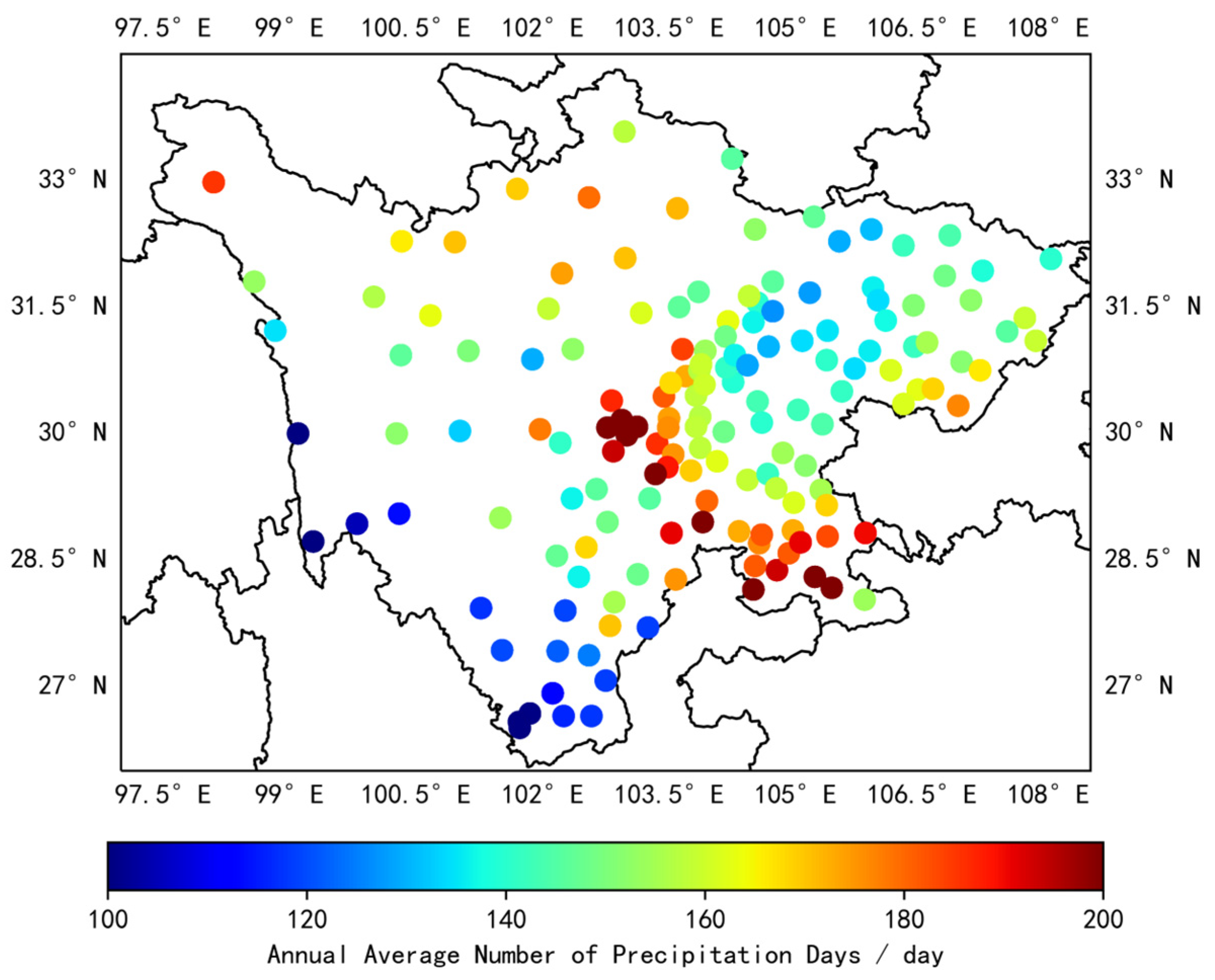
Considering both the annual average precipitation (Figure 2) and the annual average number of precipitation days (Figure 3) in the Sichuan region, it is evident that the western mountainous highlands receive less rainfall in terms of both volume and frequency than other areas. Here, the annual average precipitation was a minimum of 500 mm and the smallest average number of annual precipitation days was 100, signifying scarce rainfall in western Sichuan. In contrast, the central region, marked by complex topography at the junction of the plains and highlands, is conducive to precipitation owing to significant terrain variations. This area records a larger volume and number of rainy days, with the highest annual average precipitation of 1300 mm and 200 annual precipitation days on average. Finally, distinct precipitation patterns were observed in the eastern plains of Sichuan. The central plains experience noticeably less rainfall than the surrounding regions, with the annual average precipitation ranging from 800 to 1000 mm, which is slightly higher than that of the western highlands. In contrast, the northeastern plains registered fewer rainfall days but higher rainfall volumes, indicating the occurrence of intense rainfall events, thus indicating that this region is prone to heavy rainfall episodes.

4.2. Temporal Distribution Characteristics of Annual Precipitation in Sichuan

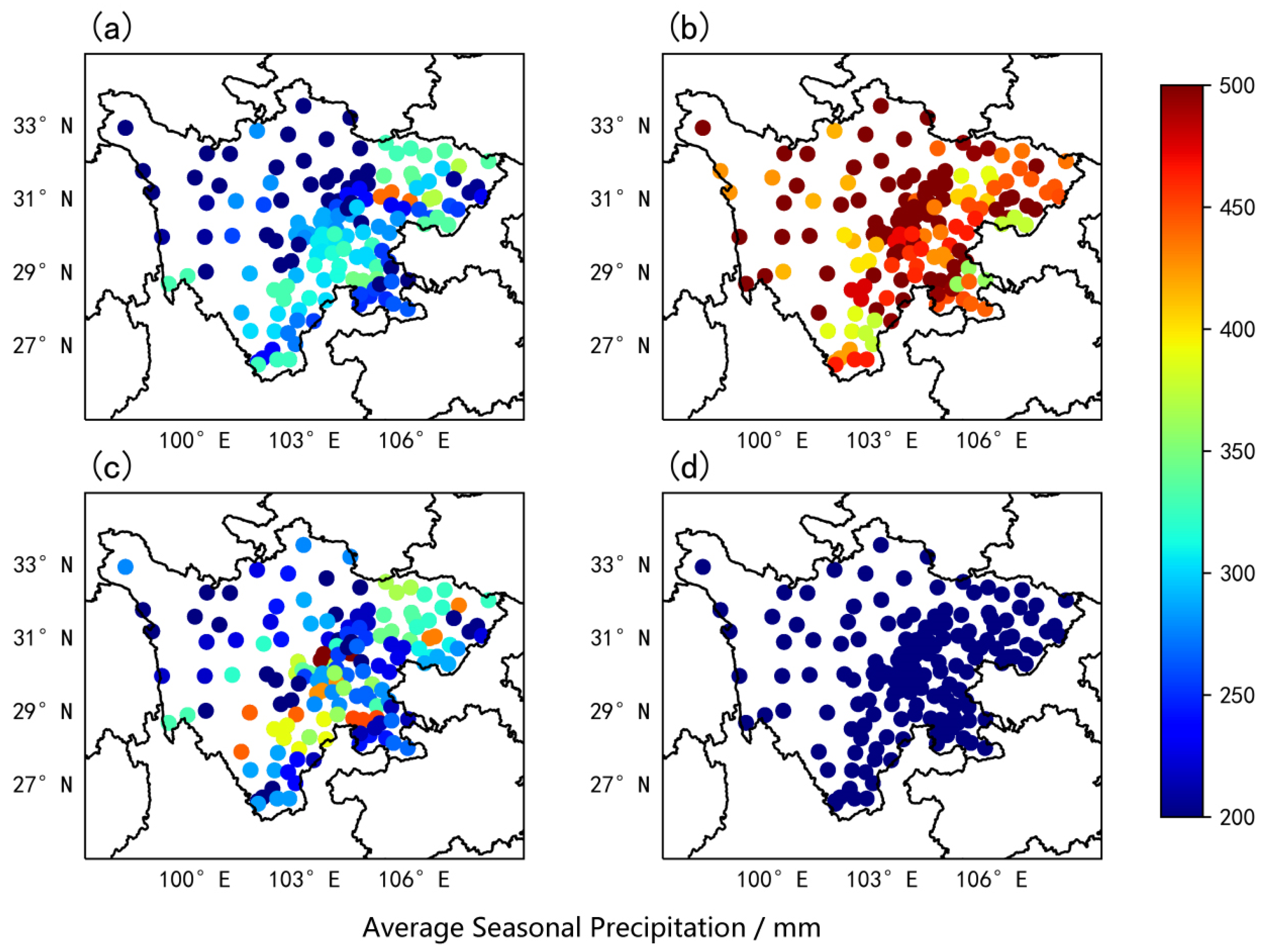
The observational data of seasonal average precipitation (Figure 4) showed that summer received the highest amount of rainfall, reaching over 500 mm, while winter received the lowest, at approximately 200 mm. The precipitation distribution during spring and autumn was uneven, with discernible concentration centers represented by the Daba Mountain and Western Sichuan rain screen belts. When comparing these observational results with the forecast data (Figure 5), the temporal analysis suggests that winter forecasts show the highest concurrence and smallest error, whereas summer forecasts demonstrate the lowest concurrence and the most significant error. Spatially, the complex terrain at the junction of the plains and highlands in Sichuan revealed the largest forecast errors, with a noticeable underestimation in precipitation predictions, whereas in the central plains, forecasts tended to overestimate rainfall. These two areas exhibited the most significant error distributions, whereas the western highland mountainous area exhibited smaller and more unevenly distributed errors.

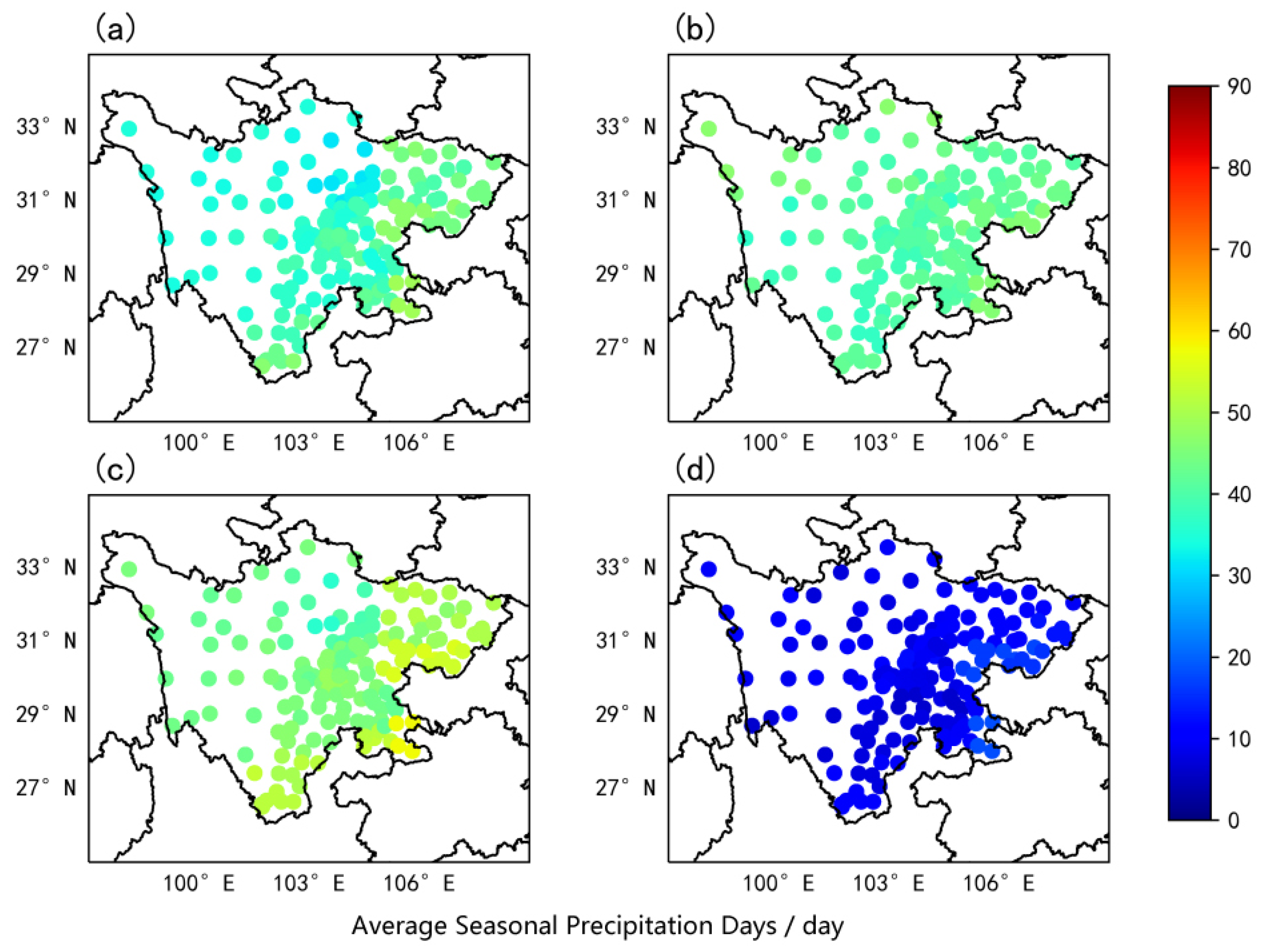
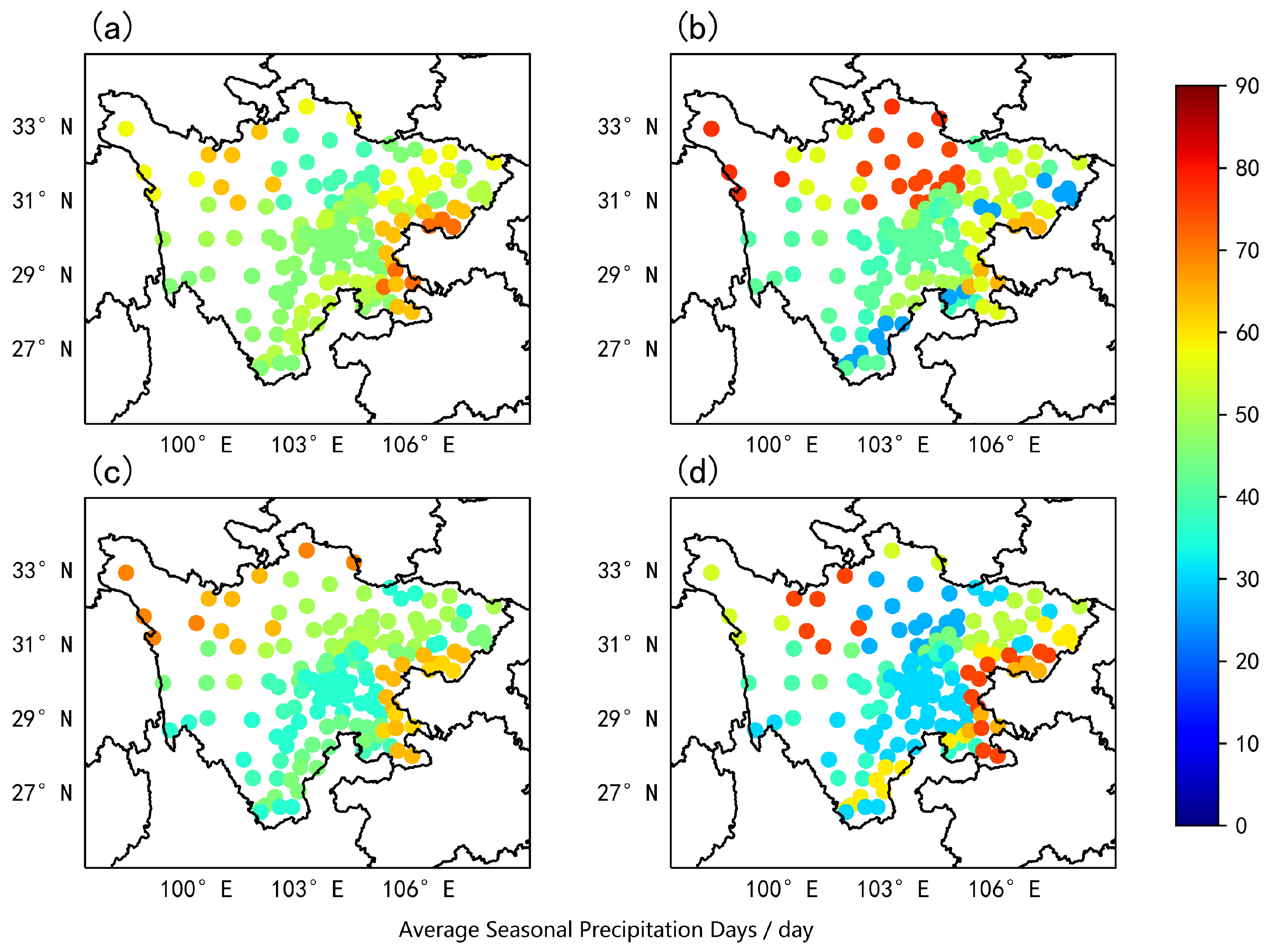
The observational data of average precipitation days per season (Figure 6) showed that autumn had the most rainy days, exceeding 55, whereas winter had the fewest at less than 10. Coupled with the analysis of average rainfall, it is evident that autumn has frequent rainfall with less precipitation per event, signifying persistent autumn rain. In contrast, summer experiences fewer rainfall events but with higher precipitation per event and is thus more prone to short-term heavy rainfall. Combining observational and forecast data (Figure 7), from a temporal perspective, winter showed the worst concurrence, whereas autumn demonstrated the best. Spatially, the overall forecasts of the Sichuan region are predominantly overestimated but the overestimation is most prominent in the central plains and northern highlands, with the error magnitude typically decreasing from the east–west extremes towards the center.

In summary, from a temporal perspective, summer forecasts presented the most significant errors, whereas winter forecasts presented the fewest. From a spatial viewpoint, the central complex terrain of the Sichuan region had the largest number of forecast errors, whereas the western highland mountainous area had the smallest.

5. Analysis of Analog Ensemble Method Application Results

5.1. Temporal Sequence Effectiveness Evaluation

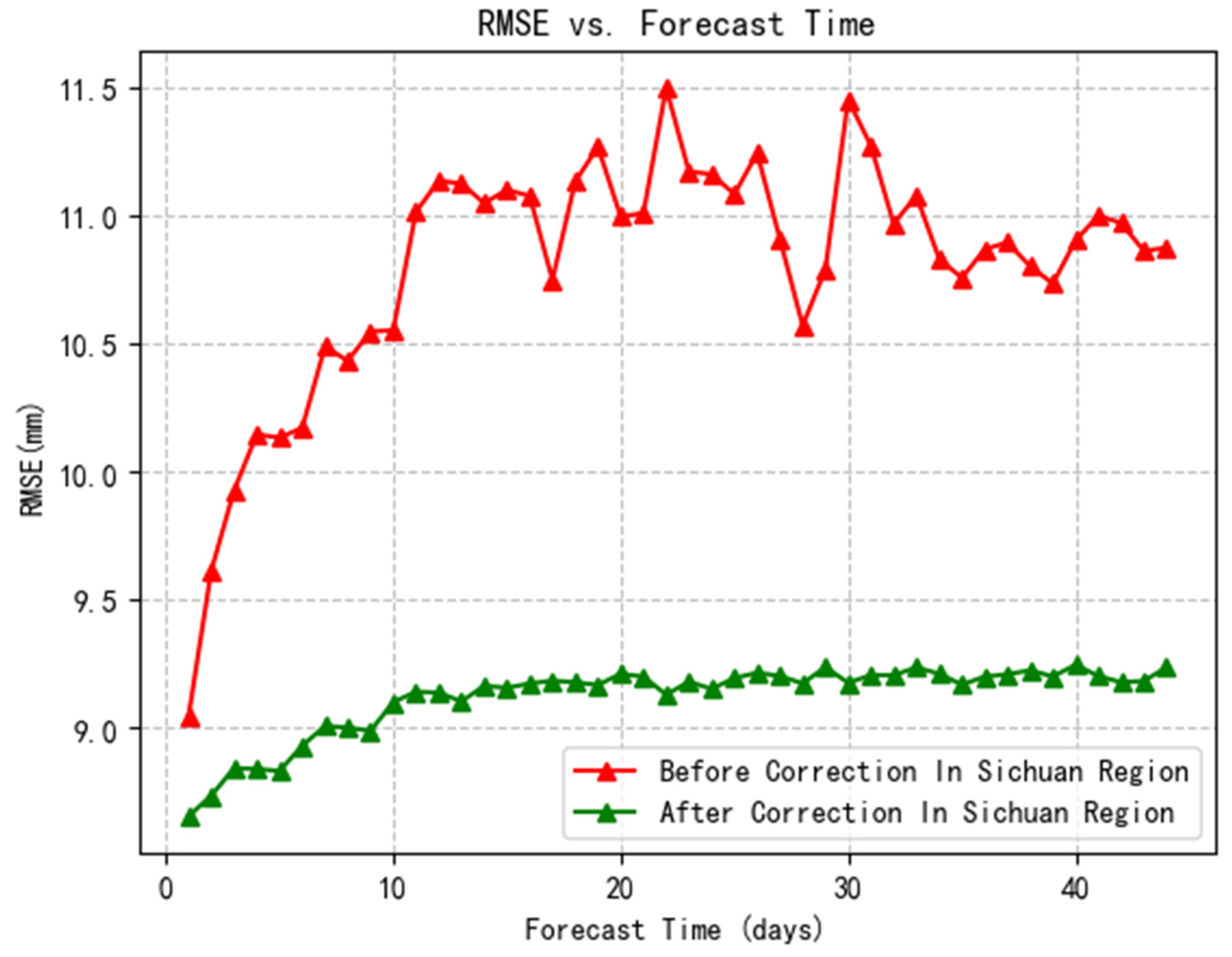
An examination of the forecast results for the average precipitation in Sichuan over the next 44 days using the CFSv2 model before and after correction (Figure 8) demonstrated improved forecast performance after correction, regardless of the forecast extension period. The RMSE was used as the evaluation metric, using the initial forecast times for each season from 2019 to 2020. The RMSE before correction ranged from 9 to 11.5 mm, whereas the RMSE after correction decreased by approximately 2 mm after correction. Before correction, the RMSE increased sharply within the first 15 days of the forecast period, with a minimum RMSE of 9 mm on day 1 and 11 mm on day 15. Subsequently, the rate of the RMSE increase slowed and oscillated at approximately 11 mm. After correction, the RMSE was significantly reduced to less than 9.5 mm and the rate of change was similar to that before correction. The RMSE increased rapidly within the first 10 days, then slowed and remained relatively stable at approximately 9.2 mm. The AnEn algorithm effectively reduced the model’s forecast error and partially mitigated the negative impact of increasing errors owing to the extension of the forecast period.

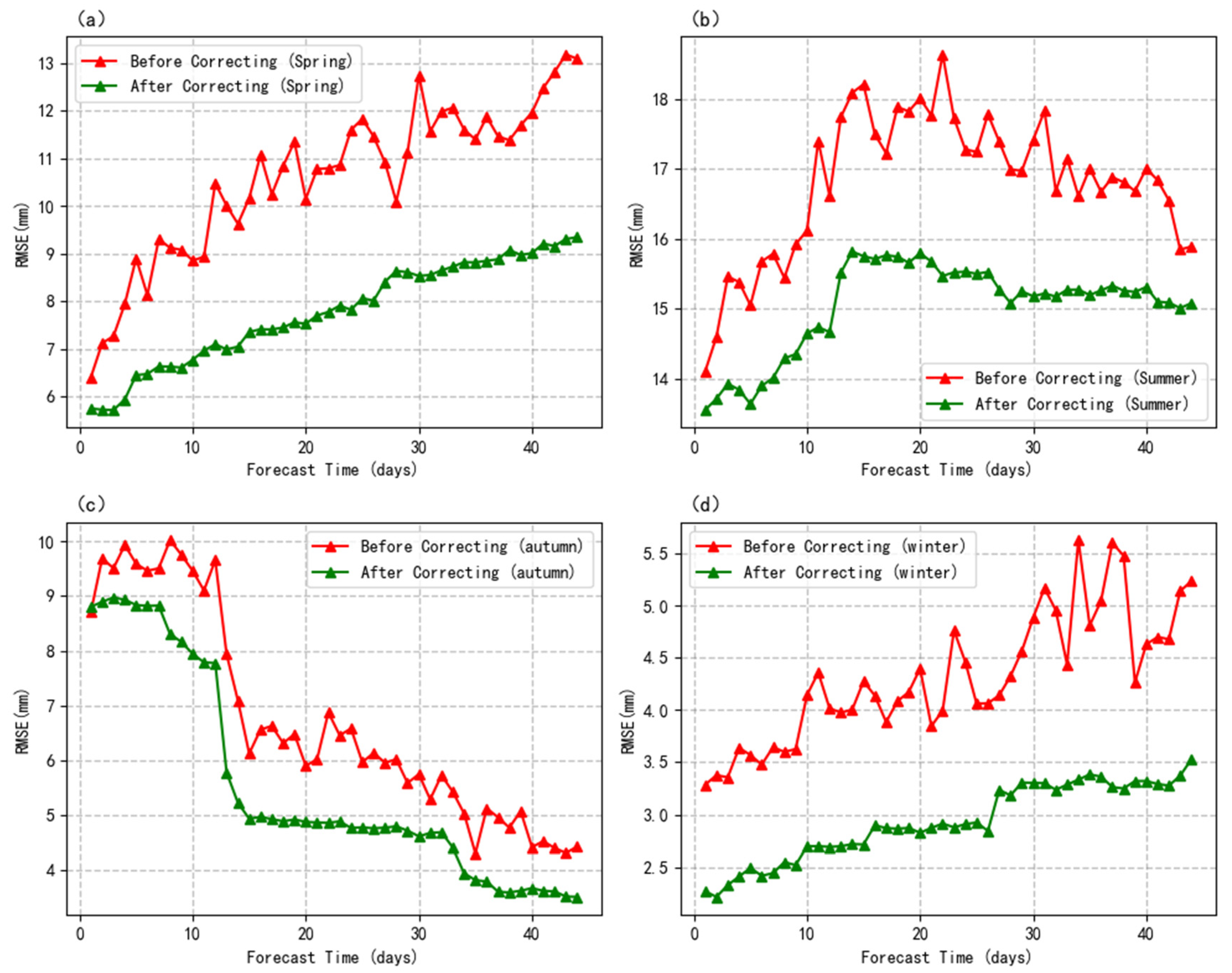
In terms of the precipitation forecasts before and after correction for different seasons (Figure 9), the corrected forecasts were superior regardless of the season. However, the number of errors was the largest in summer, smallest in winter, and intermediate in spring and autumn. The correction effect was the best in spring and summer, with the error reduction reaching 3–4 mm, whereas the effect was slightly weaker in autumn and winter, at approximately 1–2 mm. As the forecast extension period lengthened, the error growth rate increased in spring and winter, with an overall upward trend, whereas a downward trend was observed in summer and autumn. In autumn, before correction, the RMSE decreased sharply from 9.5 mm to approximately 6 mm after 11 days of the forecast period and then slowly declined to its minimum value of 4.5 mm at a forecast period of 40 days. After correction, the error trend remained unchanged, with an overall reduction of approximately 1 mm. In summer, both before and after correction, the error size reached a turning point at approximately 15 days of the forecast period, followed by a general downward trend. The correction effect improved after 15 d.

It is noteworthy that compared with the entire period, summer and autumn exhibited a different trend: the RMSE gradually decreased with the extension of the forecast period. We found that owing to the distinct precipitation patterns in different seasons in the Sichuan area, there were substantial differences in the error of model forecasts for each season. Specifically, the RMSE in autumn was lower than that in summer and that in winter was lower than that in autumn. As the forecast period extended, the actual forecast time approached the next season, resulting in a decreasing RMSE trend in summer and autumn over time. To some extent, this substantiates the significant differences in the errors of the model forecasts during different seasons in the Sichuan area.

5.2. Investigation of Precipitation Events across Varying Magnitudes

The results from the CFSv2 precipitation forecast indicate that the highest forecast error was observed in summer, followed by spring, autumn, and winter (Figure 9). However, when considering the correction effects (Figure 10), the most substantial improvement was observed in the spring precipitation forecast, whereas the correction for the summer forecast tended to be less effective. Considering the climatic characteristics of the Sichuan region, it can be postulated that the disparities between the forecast and correction results across different seasons are primarily attributed to the variable performance of the CFS model and AnEn algorithm in response to different precipitation amounts.

We classified the precipitation samples from 2017 to 2020 in the Sichuan region according to the daily rainfall levels into three classes: less than 10 mm (light rain), 10–25 mm (moderate rain), and greater than 25 mm (heavy rain). We then calculated the RMSE for the precipitation processes of different categories to compare the discrepancies in the forecasting performance of the CFS model and AnEn method. As shown in Figure 11, the largest forecasting error occurred in the prediction of heavy rain, followed by moderate and light rain. This trend suggests that the accuracy of the CFS model deteriorates as the rainfall amount increases. This observation may explain the larger errors observed during the summer season, which is typically characterized by frequent heavy rain in Sichuan, whereas lighter and moderate rain predominate in other seasons.

Considering the correction effects for different rainfall levels, the prediction accuracy for light rain improved notably after correction and the correction effect closely mirrored the effect observed when rainfall events were not categorized. This correlation may have been due to the high proportion of light rain events in Sichuan. However, for moderate and heavy rain events, the correction effects were less successful. In some instances, the forecast errors increased post-correction, explaining the poor correction outcomes observed in summer, a season with larger forecast errors.

From these results, we conclude that the diverse results produced by the model forecast and AnEn algorithm across different seasons primarily stem from their varied performance in predicting different levels of precipitation events.

5.3. Spatial Distribution Evaluation

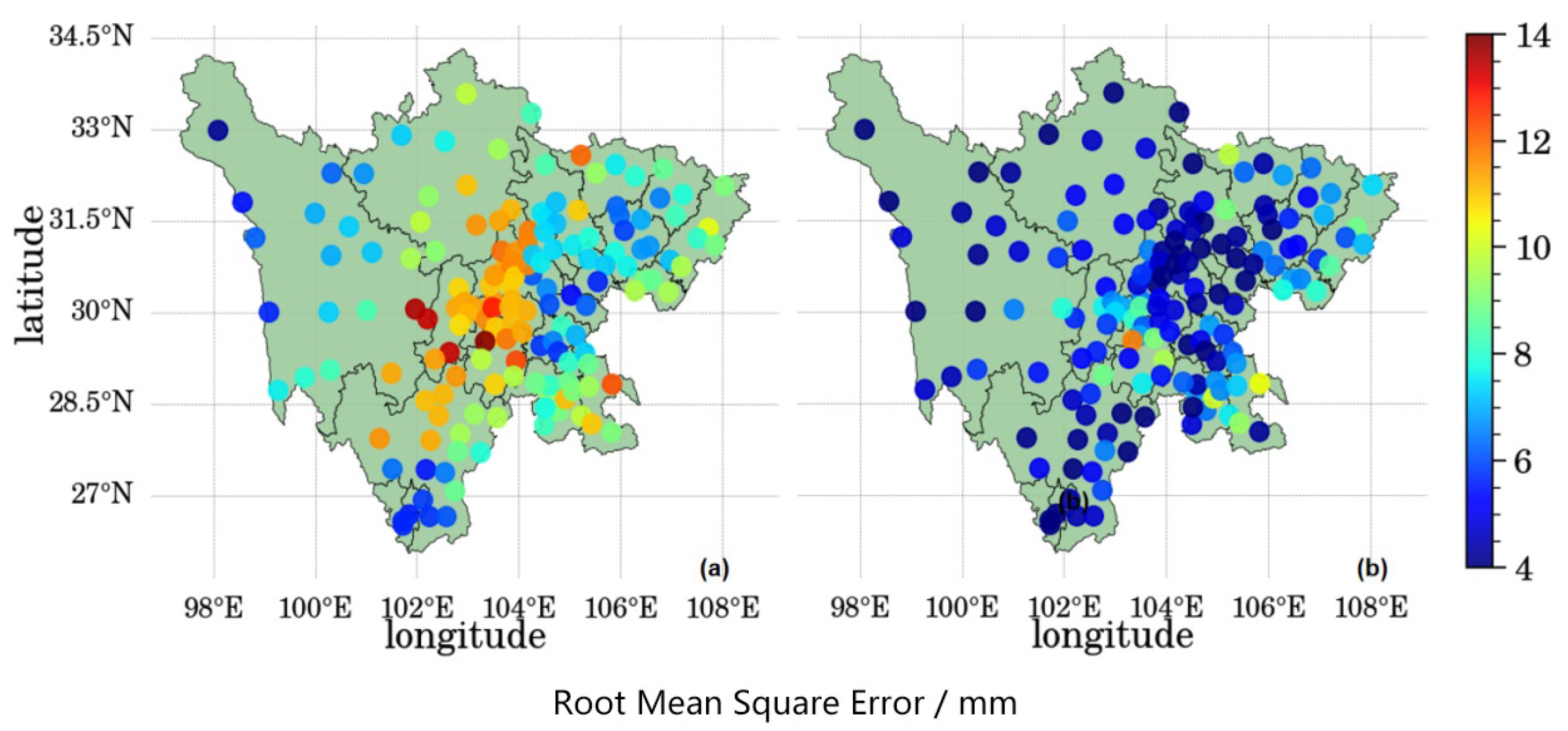
Figure 12 presents the RMSE of the accumulated precipitation on 14 October 2019, before and after correction for 156 observation stations. Overall, the AnEn method significantly reduced the RMSE of the CFSv2 precipitation data. Before correction, the RMSE in some regions exceeded 10 mm, particularly in areas with dramatic topographic changes in central Sichuan. After correction, the RMSE for most station locations was reduced to 4 mm; for some central stations, the reduction reached 10 mm. In contrast, a few stations near the western Sichuan Basin experienced a higher RMSE after correction and the reduction was smaller than that at the other stations. Additionally, there were a few stations in eastern Sichuan where a comparison between the pre- and post-correction effects was not evident.

Considering the impact of observational data on model results, it is worth noting that the pre-correction CFSv2 RMSE indicates a poorer forecast performance in central Sichuan, where stations are densely distributed, compared to that in western Sichuan, which has a sparse station distribution. At some central Sichuan stations, the error reached 14 mm, whereas the stations in eastern Sichuan exhibited consistently good forecasting data. Considering that central Sichuan serves as a boundary between complex and non-complex regions with rapidly decreasing terrain, it is expected to have a significant influence on the model forecast results.

In the preceding sections, we revised the model forecasts for all four seasons from 2019–2020. To more intuitively demonstrate the degree of improvement that the AnEn corrections have imparted to rainfall predictions in the Sichuan area, we calculated the RMSE before and after corrections for each forecast initiation time across the four seasons. We selected the day with the greatest reduction in RMSE post-correction, comparing the forecast results 1 day and 44 days before and after correction with the observed data. Specifically, we chose the rainfall forecast initiated on 30 May 2019, with a forecast period of 1 day (Figure 13). To contrast the varying effects of the model corrections for different forecast durations, we also selected the daily rainfall volume forecast initiated on May 30, 2019, with a forecast period of 44 days (Figure 14).

As observed from the figures, the primary rainfall regions during this period were situated in the western and northeastern parts of the plains, with sporadic rainfall areas in southern Sichuan. Before correction, the model forecasts significantly overestimated the precipitation, resulting in pronounced over-forecasting. The errors were primarily concentrated in areas with complex topography in the southern highlands and at the border, with a maximum error exceeding 10 mm. Concurrently, under-forecasting was observed in the northeastern plains, particularly around the Daba Mountains. After correction, the forecasted rainfall regions were more accurate although the forecasted area was larger than the actual area. However, the over-forecasting issue in areas with complex topography had been broadly corrected. As a practical reference for actual forecasting, the corrected model forecast provides more precise cues regarding rainfall locations than the pre-correction forecast.

With the extension of the forecast period, the model forecast errors notably increased. Apart from minor areas in the southern and northern highlands, over-forecasting occurred throughout Sichuan, with a maximum error exceeding 10 mm. After correction, over-forecasting was substantially improved, reducing the error to approximately 5 mm. Furthermore, the rainfall area originally located in the southwestern highlands was more accurately forecasted after correction despite reductions in intensity and range. Simultaneously, the forecast results for the rainfall area in the southeastern plains shifted westward and over-forecasting in the northeastern plains showed limited improvement. To some extent, this evidence confirms the phenomenon of diminishing correction effectiveness with forecast period extension.

5.4. Overall Performance Evaluation

To assess the accuracy of the CFSv2 model in forecasting precipitation before and after correction, Figure 15 compares the CFSv2 model results with the AnEn-corrected model results and selects two different forecast lead times of 1 and 40 days, ultimately quantifying the results using a Taylor diagram [50]. Overall, the results indicate that the corrected model forecasts are significantly better than those of the original CFSv2 model, with both lead times showing an increase of more than 0.1 in spatial correlation coefficients, and a significant reduction in root-mean-square error, with a decrease of up to 6 mm. The corrected standard deviation closely resembled the standard deviation of the observed data. The correction results show some differences when both forecast lead times are considered. The correction result for a 1-day lead time was significantly better than that for a 40-day lead time, with the standard deviation of the 1-day lead-time correction result being nearly identical to the observed value, a spatial correlation coefficient increase of approximately 0.1, and a root-mean-square error reduction of approximately 0.6. Based on the three evaluation metrics, it can be concluded that the correction effect gradually worsens as the forecast lead time increases.

6. Discussion and Considerations

This study utilized daily CFSv2 surface precipitation forecasts for 44 days ahead from 2017 to 2020 and employed the AnEn algorithm to construct a precipitation prediction experiment for 0–44 days forecasts, comparing the corrected model results with observed data. Daily precipitation observations from 156 meteorological stations in Sichuan Province from 2017 to 2020 were used to statistically analyze the spatiotemporal distribution characteristics of precipitation in different seasons. The following conclusions were drawn:

• In terms of spatial distribution, the amount of precipitation and rainy days in Sichuan Province generally decreased from east to west. Mountainous regions received higher annual precipitation with a more uniform distribution, whereas hilly and basin regions had an uneven precipitation distribution. In contrast, the plains and basins experienced a more consistent distribution of precipitation with an increased number of rainy days. As for the temporal distribution, autumn recorded the highest number of rainy days, while summer showed the maximum precipitation with continuous autumn rain and short-duration heavy rain.
• The AnEn algorithm improved the accuracy of extended-range precipitation forecasts for different seasons in Sichuan Province, significantly reducing the RMSE of the CFSv2 forecast results. Correction of the model forecast results significantly improved the precipitation forecasting in the region.
• To investigate the causes of varying correction effects in different seasons, we conducted a stratified study on precipitation. We found that the primary reason lay in the differing performances of the CFS model and AnEn correction method in relation to precipitation events at various levels. Notably, the CFS model and AnEn correction method exhibited the poorest performance in the context of heavy rainfall events.
• The effectiveness of the AnEn method in improving the model forecasting ability varies depending on the initial and forecast lead times in different seasons. Generally, the correction effect was more pronounced in spring and summer than in autumn and winter. Furthermore, short-term forecast lead times exhibited better correction effects than long-term forecast lead times. However, individual stations may exhibit suboptimal correction results.

The applicability of this study is limited because it focused only on the Sichuan Basin. Additionally, some stations may continue to demonstrate considerable errors in the corrected forecasts. Future research should consider expanding the study area and applying and validating the AnEn method in other regions. Furthermore, exploring the combination of other methods to improve precipitation forecasting accuracy in complex terrains could be beneficial.

References

1. Qian, T.; Zhao, P.; Zhang, F.; Bao, X. Rainy-Season Precipitation over the Sichuan Basin and Adjacent Regions in Southwestern China. Mon. Weather Rev. 2015, 143, 383–394. [Google Scholar] [CrossRef]
2. Vitart, F.; Molteni, F. Simulation of the Madden-Julian Oscillation and its teleconnections in the ECMWF forecast system. Q. J. R. Meteorol. Soc. 2010, 136, 842–855. [Google Scholar] [CrossRef]
3. Benjamin, S.G.; Weygandt, S.S.; Brown, J.M.; Hu, M.; Alexander, C.R.; Smirnova, T.G.; Olson, J.B.; James, E.P.; Dowell, D.C.; Grell, G.A.; et al. A North American Hourly Assimilation and Model Forecast Cycle: The Rapid Refresh. Mon. Weather Rev. 2016, 144, 1669–1694. [Google Scholar] [CrossRef]
4. Bauer, P.; Thorpe, A.; Brunet, G. The quiet revolution of numerical weather prediction. Nature 2015, 525, 47–55. [Google Scholar] [CrossRef]
5. Ming, X.; Liang, Q.; Xia, X.; Li, D.; Fowler, H.J. Real-Time Flood Forecasting Based on a High-Performance 2-D Hydrodynamic Model and Numerical Weather Predictions. Water Resour. Res. 2020, 56, e2019WR025583. [Google Scholar] [CrossRef]
6. Efstathiou, G.A.; Zoumakis, N.M.; Melas, D.; Lolis, C.J.; Kassomenos, P. Sensitivity of WRF to boundary layer parameterizations in simulating a heavy rainfall event using different microphysical schemes. Effect on large-scale processes. Atmos. Res. 2013, 132–133, 125–143. [Google Scholar]
7. Tudor, M.; Ivatek-Šahdan, S.; Stanešić, A.; Horvath, K.; Bajić, A. Forecasting weather in Croatia using ALADIN numerical weather prediction model. In Climate Change and Regional/Local Responses; IntechOpen: London, UK, 2013. [Google Scholar]
8. White, C.; Franks, S.; McEvoy, D. Using subseasonal-to-seasonal (S2S) extreme rainfall forecasts for extended-range flood prediction in Australia. Proc. Int. Assoc. Hydrol. Sci. 2015, 370, 229–234. [Google Scholar]
9. Lang, L.C.; Tang, C.; Gao, X.; Li, Z.H.; Wu, F. Spatial interpolation of high-resolution daily precipitation over complex terrains. Acta Geogr. Sin. 2023, 78, 101–120. [Google Scholar]
10. Zhao, P.W.; Li, B.; Wang, J.N.; Yang, H.Q.; Guo, P.; Gong, L.J. Accuracy Evaluation and Comparison of GPM IMERG and ERA5 Precipitation Products over Complex Terrain of Yunnan. Meteorol. Sci. Technol. 2021, 49, 114–123. [Google Scholar]
11. Chen, F.L.; Liu, X.T.; Zeng, D.D.; Jiang, S.; Gan, Q.; Liang, J.J. Effect of topography on a warm-sector heavy rainfall event in the northern pearl river delta. J. Trop. Meteorol. 2022, 38, 377–386. [Google Scholar]
12. De Giorgi, M.G.; Ficarella, A.; Tarantino, M. Assessment of the benefits of numerical weather predictions in wind power forecasting based on statistical methods. Energy 2011, 36, 3968–3978. [Google Scholar] [CrossRef]
13. Delle Monache, L.; Nipen, T.; Liu, Y.; Roux, G.; Stull, R. Kalman filter and analog schemes to postprocess numerical weather predictions. Mon. Weather Rev. 2011, 139, 3554–3570. [Google Scholar] [CrossRef] [Green Version]
14. Falck, A.S.; Tomasella, J.; Diniz, F.L.R.; Maggioni, V. Applying a precipitation error model to numerical weather predictions for probabilistic flood forecasts. J. Hydrol. 2021, 598, 126374. [Google Scholar] [CrossRef]
15. Zhao, X.; Liu, J.; Yu, D.; Chang, J. One-day-ahead probabilistic wind speed forecast based on optimized numerical weather prediction data. Energy Convers. Manag. 2018, 164, 560–569. [Google Scholar] [CrossRef]
16. Nandar, A. Bayesian network probability model for weather prediction. In Proceedings of the 2009 International Conference on the Current Trends in Information Technology (CTIT), Dubai, United Arab Emirates, 15–16 December 2009; IEEE: Piscataway, NJ, USA, 2009; pp. 1–5. [Google Scholar]
17. Zhao, H.S.; Jin, L.; Huang, X.Y.; Huang, Y. Ecmwf precipitation grading correction forecast method based on cnn and rf algorithm. Meteorol. Sci. Technol. 2021, 49, 419–426. [Google Scholar]
18. Delle Monache, L.; Eckel, F.A.; Rife, D.L.; Nagarajan, B.; Searight, K. Probabilistic Weather Prediction with an Analog Ensemble. Mon. Weather Rev. 2013, 141, 3498–3516. [Google Scholar] [CrossRef] [Green Version]
19. van den Dool, H.M. A New Look at Weather Forecasting through Analogues. Mon. Weather Rev. 1989, 117, 2230–2247. [Google Scholar] [CrossRef]
20. Panziera, L.; Germann, U.; Gabella, M.; Mandapaka, P.V. NORA-Nowcasting of Orographic Rainfall by means of Analogues. Q. J. R. Meteorol. Soc. 2011, 137, 2106–2123. [Google Scholar] [CrossRef]
21. Hamill, T.M.; Whitaker, J.S. Probabilistic Quantitative Precipitation Forecasts Based on Reforecast Analogs: Theory and Application. Mon. Weather Rev. 2006, 134, 3209–3229. [Google Scholar] [CrossRef]
22. Cervone, G.; Clemente-Harding, L.; Alessandrini, S.; Delle Monache, L. Short-term photovoltaic power forecasting using Artificial Neural Networks and an Analog Ensemble. Renew. Energy 2017, 108, 274–286. [Google Scholar] [CrossRef] [Green Version]
23. Hu, W.; Cervone, G. Dynamically Optimized Unstructured Grid (DOUG) for Analog Ensemble of numerical weather predictions using evolutionary algorithms. Comput. Geosci. 2019, 133, 104299. [Google Scholar] [CrossRef]
24. Junk, C.; Delle Monache, L.; Alessandrini, S.; Cervone, G.; von Bremen, L. Predictor-weighting strategies for probabilistic wind power forecasting with an analog ensemble. Meteorol. Z. 2015, 24, 361–379. [Google Scholar] [CrossRef]
25. Zhang, X.; Alexander, L.; Hegerl, G.C.; Jones, P.; Tank, A.K.; Peterson, T.C.; Trewin, B.; Zwiers, F.W. Indices for monitoring changes in extremes based on daily temperature and precipitation data. WIREs Clim. Chang. 2011, 2, 851–870. [Google Scholar] [CrossRef]
26. Zhai, P. On changes of China’s maximum and minimum temperature in 1951–1990. Acta Meteorol. Sin. 1999, 13, 190. [Google Scholar]
27. Saha, S.; Moorthi, S.; Wu, X.; Wang, J.; Nadiga, S.; Tripp, P.; Behringer, D.; Hou, Y.T.; Chuang, H.Y.; Iredell, M.; et al. The NCEP Climate Forecast System Version 2. J. Clim. 2014, 27, 2185–2208. [Google Scholar] [CrossRef]
28. Alessandrini, S.; Sperati, S.; Delle Monache, L. Improving the Analog Ensemble Wind Speed Forecasts for Rare Events. Mon. Weather Rev. 2019, 147, 2677–2692. [Google Scholar] [CrossRef]
29. Gneiting, T. Making and Evaluating Point Forecasts. J. Am. Stat. Assoc. 2012, 106, 746–762. [Google Scholar] [CrossRef] [Green Version]
30. Alessandrini, S. Predicting Rare Events of Solar Power Production with the Analog Ensemble. Sol. Energy 2022, 231, 72–77. [Google Scholar] [CrossRef]
31. Alaoui, B.; Bari, D.; Bergot, T.; Ghabbar, Y. Analog Ensemble Forecasting System for Low-Visibility Conditions over the Main Airports of Morocco. Atmosphere 2022, 13, 1704. [Google Scholar] [CrossRef]
32. Candido, S.; Singh, A.; Delle Monache, L. Improving Wind Forecasts in the Lower Stratosphere by Distilling an Analog Ensemble Into a Deep Neural Network. Geophys. Res. Lett. 2020, 47, e2020GL089098. [Google Scholar] [CrossRef]
33. Raman, A.; Arellano, A.F.; Delle Monache, L.; Alessandrini, S.; Kumar, R. Exploring Analog-Based Schemes for Aerosol Optical Depth Forecasting with WRF-Chem. Atmos. Environ. 2021, 246, 118134. [Google Scholar] [CrossRef]
34. Jeworrek, J.; West, G.; Stull, R. Optimizing Analog Ensembles for Sub-Daily Precipitation Forecasts. Atmosphere 2022, 13, 1662. [Google Scholar] [CrossRef]
35. Sha, Y.; Gagne, D.J., II; West, G.; Stull, R. A hybrid analog-ensemble, convolutional-neural-network method for post-processing precipitation forecasts. Mon. Weather. Rev. 2022, 150, 1495–1515. [Google Scholar] [CrossRef]
36. Alessandrini, S.; Delle Monache, L.; Rozoff, C.; Lewis, W. Probabilistic Prediction of Hurricane Intensity with an Analog Ensemble. In Proceedings of the 96th American Meteorological Society Annual Meeting, New Orleans, LA, USA, 10–14 January 2016. [Google Scholar]
37. Ren, F.; Ding, C.; Zhang, D.L.; Chen, D.; Ren, H.L.; Qiu, W. A Dynamical-Statistical-Analog Ensemble Forecast Model: Theory and an Application to Heavy Rainfall Forecasts of Landfalling Tropical Cyclones. Mon. Weather Rev. 2020, 148, 1503–1517. [Google Scholar] [CrossRef]
38. Keller, J.D.; Monache, L.D.; Alessandrini, S. Statistical Downscaling of a High-Resolution Precipitation Reanalysis Using the Analog Ensemble Method. J. Appl. Meteorol. Climatol. 2017, 56, 2081–2095. [Google Scholar] [CrossRef]
39. Willmott, C.; Matsuura, K. Advantages of the mean absolute error (MAE) over the root mean square error (RMSE) in assessing average model performance. Clim. Res. 2005, 30, 79–82. [Google Scholar] [CrossRef]
40. Zhi, X.F.; Wang, S.S.; Zhou, H.M.; Zhu, S.P.; Zhao, H. Statistical downscaling of precipitation forecasting using categorized rainfall regression. Trans. Atmos. Sci. 2016, 39, 329–338. [Google Scholar] [CrossRef]
41. Shao, D.; Zhang, Y.; Xu, J.; Zhang, H.; Chen, S.; Tu, S. Comparison between Multi-Physics and Stochastic Approaches for the 20 July 2021 Henan Heavy Rainfall Case. Atmosphere 2022, 13, 1057. [Google Scholar] [CrossRef]
42. Li, J.; Heap, A.D. A review of comparative studies of spatial interpolation methods in environmental sciences: Performance and impact factors. Ecol. Inform. 2011, 6, 228–241. [Google Scholar] [CrossRef]
43. Li, J.; Heap, A.D. Spatial interpolation methods applied in the environmental sciences: A review. Environ. Model. Softw. 2014, 53, 173–189. [Google Scholar] [CrossRef]
44. Hisham, M.B.; Yaakob, S.N.; Raof, R.A.A.; Nazren, A.B.A.; Wafi, N.M. An Analysis of Performance for Commonly Used Interpolation Method. Adv. Sci. Lett. 2017, 23, 5147–5150. [Google Scholar] [CrossRef]
45. Danahy, E.E.; Agaian, S.S.; Panetta, K.A. Algorithms for the resizing of binary and grayscale images using a logical transform. Proc. Imaging Process. Algorithms Syst. 2007, 6497, 305–314. [Google Scholar]
46. Deng, L.H.; Liu, G.Q.; Li, X.B.; Song, T.F.; Huang, S.J. Applied Research of Image Zoom Based on Interpolation Algorithm. Microcomput. Inf. 2010, 26, 23–24. [Google Scholar]
47. Cheng, Y.L.; He, F.; Tan, F.F.; Wang, Z.D.; Qin, L.A.; Jing, X.; Zhang, S.L.; Hou, Z.H. Research on the laser spot restoration method of detector array target. Laser Infrared 2020, 50, 749–753. [Google Scholar]
48. Jing, Z.; Wu, L.X.; Ma, X.H. Sensitivity of near-inertial internal waves to spatial interpolations of wind stress in ocean generation circulation models. Ocean Model. 2016, 99, 15–21. [Google Scholar] [CrossRef] [Green Version]
49. Li, P.C.; Liu, X.D. Bilinear interpolation method for quantum images based on quantum Fourier transform. Int. J. Quantum Inf. 2018, 16, 1850031. [Google Scholar] [CrossRef]
50. Guo, Y.; Nie, H. Summertime daily precipitation statistics over East China in CFSv2. Phys. Chem. Earth Parts A/B/C 2020, 115, 102841. [Google Scholar] [CrossRef]
Figure 1. Distribution of meteorological stations in Sichuan Province, marked with purple dots. The figure also depicts the height of each station. The triangular region corresponds to the city of Chengdu.
Atmosphere 14 01223 g001
Figure 2. Annual average precipitation in Sichuan.
Atmosphere 14 01223 g002
Figure 3. Annual average number of precipitation days in Sichuan.
Atmosphere 14 01223 g003
Figure 4. Average seasonal precipitation in Sichuan from 2017 to 2020 ((a): spring, (b): summer, (c): autumn, (d): winter).
Atmosphere 14 01223 g004
Figure 5. Average seasonal precipitation in Sichuan from 2017 to 2020 based on CFSv2 Forecasts ((a): spring, (b): summer, (c): autumn, (d): winter).
Atmosphere 14 01223 g005
Figure 6. Average seasonal precipitation days in Sichuan from 2017 to 2020 ((a): spring, (b): summer, (c): autumn, (d): winter).
Atmosphere 14 01223 g006
Figure 7. Average seasonal precipitation days in Sichuan from 2017 to 2020 based on CFSv2 Forecasts ((a): spring, (b): summer, (c): autumn, (d): winter).
Atmosphere 14 01223 g007
Figure 8. RMSE before and after correction in Sichuan (red line represents before correction and green line represents after correction).
Atmosphere 14 01223 g008
Figure 9. RMSE before and after correction for each season in Sichuan: (a) spring, (b) summer, (c) autumn, and (d) winter; red line indicates before correction and green line indicates after correction.
Atmosphere 14 01223 g009
Figure 10. Percentage reduction in RMSE after correction across different seasons in Sichuan.
Atmosphere 14 01223 g010
Figure 11. RMSE before and after corrections for light, moderate, and heavy rain events in Sichuan: (a) overall RMSE, (b) light rain, (c) moderate rain, and (d) heavy rain. The red line represents the RMSE before corrections and the green line indicates the RMSE after corrections.
Atmosphere 14 01223 g011
Figure 12. Distribution of RMSE for CFSv2 forecast results as the field to be corrected: before correction (a) and after correction (b). The correction time is 14 October 2019, and the colored solid circles represent RMSE.
Atmosphere 14 01223 g012
Figure 13. Daily precipitation in Sichuan Province on 30 May 2019, with a forecast time limit of 1 day, in mm: (a) observed data, (b) uncorrected CFSv2 forecast results, and (c) corrected CFSv2 model forecast results.
Atmosphere 14 01223 g013
Figure 14. Daily precipitation in Sichuan Province on 30 May 2019, with a forecast time limit of 44 days, in mm: (a) observed data, (b) uncorrected CFSv2 forecast results, and (c) corrected CFSv2 model forecast results.
Atmosphere 14 01223 g014
Figure 15. Taylor diagram comparing the CFSv2 model forecast results with the AnEn-corrected model results, considering forecast lead times of 1 day (black crosses for uncorrected, black circles for corrected) and 40 days (black X for uncorrected, black squares for corrected).
Atmosphere 14 01223 g015
Disclaimer/Publisher’s Note: The statements, opinions and data contained in all publications are solely those of the individual author(s) and contributor(s) and not of MDPI and/or the editor(s). MDPI and/or the editor(s) disclaim responsibility for any injury to people or property resulting from any ideas, methods, instructions or products referred to in the content.