Comparative Analysis of Neural Network Models for Predicting Ammonia Concentrations in a Mechanically Ventilated Sow Gestation Facility in Korea

Abstract

Conventional methods for monitoring ammonia (NH₃) emissions from livestock farms have several challenges, such as a poor environment for measurement, difficulty in accessing livestock, and problems with long-term measurement. To address these issues, we applied various neural network models for the long-term prediction of NH₃ concentrations from sow farms in this study. Environmental parameters, including temperature, humidity, ventilation rate, and past records of NH₃ concentrations, were given as inputs to the models. These neural network models took the encoder or the feature extracting parts from the representative deep learning models, including Long Short-Term Memory (LSTM), Convolutional Neural Network (CNN), and Transformer, to encode temporal patterns of time series. However, all of these models adopted dense layers for the decoder to format the task of long-term prediction as a regression problem. Due to their regression nature, all models showed a robust performance in predicting long-term NH₃ concentrations at a scale of weeks or even months despite there being a relatively short period of input signals (a few days to a week). Given one week of input, LSTM showed the minimum mean absolute errors (MAE) of 1.83, 1.78, and 1.87 ppm for the prediction of one, two, and three weeks, respectively, whereas Transformer performed best with a MAE of 1.73 ppm for a four-week prediction. In the long-term estimation of spanning months, LSTM showed the minimum MAEs of 1.95 and 1.90 ppm when trained on predicting two and three weeks of windows. At the same condition, Transformer gave the minimum MAEs of 1.87 and 1.83 when trained on predicting one and four weeks of windows. Overall, the neural network models can facilitate the prediction of national-level NH₃ emissions, the development of mitigation strategies for NH₃-derived air pollutants, odor management, and the monitoring of animal-rearing environments. Further, their integration of real-time measurement devices can significantly prolong device longevity and offer substantial cost savings.

1. Introduction

Ammonia (NH₃), a colorless, toxic, corrosive, and odorous compound with high viscosity, can form fine particulate matter when converted into secondary inorganic aerosols (SIAs) such as ammonium sulfate ((NH₄)₂SO₄) and ammonium nitrate (NH₄NO₃), which are the predominant components of PM_2.5 [1,2,3,4,5,6]. Many SIAs can negatively affect ecosystems by causing visibility reduction, crop damage, and respiratory diseases [7,8,9,10,11,12,13]. NH₃ is a naturally occurring and dissipating gas; however, a significant portion is also emitted from anthropogenic activities, with large-scale livestock farming, particularly animal husbandry (manure management and fertilizer), being the primary contributor [14,15,16,17,18,19,20].

To quantify NH₃ emissions from the livestock industry, field workers and researchers from various countries have previously proposed different methods for determining the emission factors. However, owing to the unique gas-phase characteristics of NH₃, its continuous and accurate measurement has proven to be considerably more challenging compared to that of other air pollutants. For example, when measuring NH₃ emissions at a pig farm using a device with a pump, the highly viscous NH₃ may be adsorbed onto the motor, interfering with the constant velocity suction. This can introduce inaccuracies in the final concentration calculations, corrosion of the detector responsible for identifying the target substance, and reduced signal sensitivity. Therefore, the measured concentrations may significantly deviate from the actual values [21,22,23]. Furthermore, NH₃ detectors tend to be more expensive than those used for other pollutants, such as SO_x and NO_x. Further, continuous monitoring often necessitates frequent replacement in case of equipment failure, which imposes a substantial financial burden on farms and research institutes, often leading to compromised measurement and monitoring practices. Because of these limitations, the quantification of NH₃ emission requires a method that employs rapidly evolving prediction techniques relying on minimal actual measurements obtained using instruments.

Data collected from livestock farms have been extensively used to predict NH₃ concentrations using traditional methods. Notably, one approach involves the application of rigorously designed methodologies to farms capable of consistent production to determine the NH₃ emission factor per unit of activity data, thereby predicting future NH₃ emissions [24,25,26,27,28,29,30]. This approach predominantly hinges on the number of animals being reared and is highly effective for farms that maintain a systematized livestock environment along with comprehensive management systems. However, significant discrepancies can arise in small-scale facilities and irregular breeding environments. Multivariate regression models may be useful to quantify NH₃ under these conditions. These equations leverage a range of farm-collected data, including temperature, humidity, number of livestock being reared, and quantity of feed provided, along with wind direction and speed, in cases of natural ventilation [31,32,33,34]. This method can be highly effective if an equation optimized for a specific farm is derived using suitable parameters. However, as mentioned previously, this can be a costly and laborious task.

The recent success of deep learning has motivated researchers to train neural network models to predict future time-series [35,36,37,38,39,40,41,42,43]. A typical setup frames time-series prediction as a sequence-to-sequence problem wherein an input sequence is fed into a model, which is then trained to predict the output sequence. Unlike traditional machine learning methods, where features in a time series need to be engineered manually, deep learning models take raw data and automatically discover hidden patterns or features during the training process [44]. Thus, they have the advantage of discovering better data representations that are often not straightforward in traditional feature engineering. Among various neural network architectures, the recurrent neural network (RNN), or its advanced version, long short-term memory (LSTM) [45] or gated recurrent unit (GRU) [46], has been mostly tested in time-series forecasting because of its natural sequence-to-sequence nature. Other major neural network architectures such as convolutional neural networks (CNN) [47] and transformers [48] have also been used to predict time series [49,50,51]. Although these neural network models have been successful for certain settings in particular domains, their performance and characteristics have not been fully tested in integrals for long-term forecasting of time series data such as NH₃ concentrations. Therefore, we systematically trained and compared these neural network models to determine their potential applicability in predicting gas concentration time-series data.

In previous research, our team obtained high-resolution time-series data (at 2 h intervals) over a year to calculate the NH₃ emission factor of sow houses in Korea [52]. We used these data to conduct multivariate analysis for a specific period, accounting for variables such as temperature, relative humidity (RH), ventilation rate, and NH₃ concentration, and found that the characteristics and emission coefficients of NH₃ in pigsties exhibited seasonal variations, underscoring the need for representative NH₃ emission coefficients to account for these differences.

The aim of this study is to identify the most reliable model among an array of time-series deep learning models for predicting NH₃ concentrations, leveraging previously acquired datasets. Since existing NH₃ emission studies have limitations such as poor environment for measurement and difficulty in accessing livestock, it will be possible to predict long-term concentrations through some measurement data and reliable modeling, which will entail less effort and time in securing high-quality data. Given that the results produced by a model can vary significantly based on the type of data, we experimented with the application of the most commonly used models to a dataset collected from a sow farm. Unlike fattening pigs, where NH₃ concentration gradually increases as the fattening period extends, sows do not show a consistent trend of either increasing or decreasing NH₃ concentration over time. This irregular pattern makes predictions challenging with conventional models. Hence, we configured models capable of learning subtle environmental changes through deep learning, enabling the prediction of NH₃ concentration, and evaluated the performance among these models. Subsequently, the validated model was used to forecast future NH3 concentrations using a dataset with minimal measurement frequency, thereby aiding its utility in real-world agricultural contexts.

2. Materials and Methods

2.1. Pig Farm

The ventilation rate, temperature, RH, and NH₃ data used in this study were collected from a sow house in Chungcheongbuk-do, South Korea. All data were collected from 25 March 2021, to 20 January 2022. The research methodology was the same as that described by Park et al. [52]. Figure 1 presents the plan and cross-section of the experimental pig pen. The internal structures of all the rooms were identical. The numbers of breeding pigs in Rooms 1, 2, and 3 were 154, 154, and 156, respectively. Pigs with impending farrowing were moved to a farrowing pen. After farrowing and nursing, they were moved back to the sow pen. In the pigsty ventilation, air entered from the side through the mid-ceiling and was then expelled through four exhaust vents (fans) located in the interior ceiling (Figure S2). The pigsty floor comprised a 1:1 ratio of concrete to plastic-slatted flooring, with livestock manure stored in pits beneath the plastic-slatted floor. A specific amount of livestock manure was discharged every Saturday, and the slurry level was maintained at approximately 70–80% of the total capacity.

Table 1. Feed composition provided to sows during the measurement period.

Nutritional Content	Crude Protein	Crude Fat	Calcium	Phosphorus	Crude Fiber	Crude Ash	Lysine
Percentage (%)	≤13.50	≥3.00	≥0.65	≤1.50	≤8.00	≤8.00	≥0.60

shows the major components of the feed provided to the pigs during the study period.

2.2. Measurements

2.2.1. NH₃ Concentration

NH₃ was measured in real-time using photoacoustic spectroscopy (LumaSense Technologies INNOVA 1512i, Ballerup, Denmark). A multi-sampler (LumaSense Technologies INNOVA 1409 (24 ports), Ballerup, Denmark) was connected to the measuring instrument to determine the concentration in each pig house (Rooms 1–3) and in the inlet air. The NH₃ concentrations discharged from the four exhaust ports in each pigsty were also measured. The NH₃ concentration incorporated into the model was determined by subtracting the inlet air concentration (average of 0.37 ppm) from the measurements acquired individually from each room. To ensure accurate measurements, the instrument was calibrated prior to the on-site data collection using high-purity nitrogen (Rigas 99.999%, Daejeon, Republic of Korea) and NH₃ standard gas (Rigas 12.5, 25, and 50 μmol/mol, Daejeon, Republic of Korea). Consequently, the error rate between the reference point concentration and the measured value was approximately 1.5%, the R² value was 0.9998 (Figure S3), and the method detection limit (MDL) of the measuring instrument was 0.2 ppm.

2.2.2. Ventilation Rate

A small ventilation rate-measuring device (VelociCalc Air Velocity Meter 9535, TSI, USA) was constructed in accordance with the standards of the American Society of Heating, Refrigerating, and Air-Conditioning Engineers (ASHRAE). After attaching the device to a fan (Vostermans Ventilation BV Multifan 4E50 (Ø630), Venlo, the Netherlands), the actual flow rate (m³/h) for each pen was measured [53]. In the experimental pigsty, the ventilation fan was not operated at <30%. The measured ventilation at the operating rates of 30%, 50%, 70%, and 100% was used to calculate the representative values [30]. Because the ventilation fan in the pigsty operated in 1% increments, the logistic curve proposed by Jo et al. [30] was applied to estimate the ventilation rate in the missing intervals (31–49%, 51–69%, and 71–99%) compared to that in the actual measurements.

2.2.3. Temperature and RH

For the internal temperature of the pigsty and the operating rate of the ventilation fan, the 1 h average value of the data collected using the in-house sensor (1 reading/min) installed in the pigsty was utilized. The dew point measured using photoacoustic spectroscopy was applied to the dew point-relative humidity conversion formula to determine the final internal RH [54]. The conversion formula used is as presented in Equation (1).

$${\mathrm{T}}_{\mathrm{d}\mathrm{e}\mathrm{w}}=\frac{\lambda \times \left\{\ln \left(\frac{\mathrm{R}\mathrm{H}}{100}\right)+\frac{\mathsf{\beta }\times \mathrm{T}}{\mathsf{\lambda }+\mathrm{T}}\right\}}{\mathsf{\beta }-\left\{\ln \left(\frac{\mathrm{R}\mathrm{H}}{100}\right)+\frac{\mathsf{\beta }\times \mathrm{T}}{\mathsf{\lambda }+\mathrm{T}}\right\}}$$

(1)

T: Temperature in pig room (−45 °C < T < 60 °C);

RH: Relative humidity (%);

$\mathsf{\beta }$: 17.62;

$\mathsf{\lambda }$: 243.12 °C.

The NH₃ concentration, ventilation rate, temperature, and relative humidity data are detailed in the Supplementary Materials (Figure S1).

2.3. Models

We first preprocessed the collected time-series data, set up baseline and neural network models, and then cross-validated the models to estimate their performance on predicting NH₃ concentrations. The pipeline of our analysis is outlined in Figure 2.

2.3.1. Data Preprocessing

Data blocks. All the data used were aggregated at 2 h intervals, which served as the NH₃ collection interval. For each room, the NH₃ concentrations from multiple sensors (four in Rooms 1 and 3, and three in Room 2) were averaged to obtain a single time series. The entire time series was then divided into several pieces or “blocks.” A block of data contained consecutive data points within a certain period. Of these multiple blocks, the two longest blocks were chosen for subsequent analysis, and the rest were discarded. The reason for this block selection was to ensure long consecutive data points for testing long-term forecasting within each block. Figure 3 shows the average NH₃ concentrations of the two longest blocks (the summer and the winter blocks) in the three rooms. The summer blocks spanned from late March to early October 2021, and the winter blocks ranged from late October 2021 to late January 2022. The lengths (in terms of time points of 2 h intervals) of the summer blocks were 2301, 2299, and 2298 for Room 1, 2, and 3, respectively. The winter blocks were of the same length (991) in all the three rooms. The presence of voids in the central region can be attributed to the remediation process of the measurement apparatus.

Data statistics. At each time point in the time series, four features were considered: the NH₃ concentration, ventilation rate, temperature, and RH.

Table 2. Data statistics of collected data, including average, minimum, maximum, and total data average values. The following values represent the calculated quantities obtained during the summer (25 March–7 October 2021) and the winter (29 October 2021–20 January 2022) periods.

		Collected Data from Pig House
		NH3 (ppm)	Ventilation Rate (m3/h)	Temp. (°C)	RH (%)
Room 1	Avg.	10.4	2387.4	22.6	65.7
	Min.	2.6	910.6	17.0	21.9
	Max.	36.1	4806.3	32.0	100.0
Room 2	Avg.	11.7	2598.8	22.7	63.5
	Min.	2.5	910.6	18.8	20.2
	Max.	40.4	4538.3	31.5	100.0
Room 3	Avg.	11.6	2809.0	23.4	65.4
	Min.	2.6	910.6	18.6	22.6
	Max.	40.1	5214.6	33.3	100.0
Grand Average		11.2	2598.4	22.9	64.8

and Figure S4 summarize the basic statistics for the values of these features. The statistics were calculated across the summer and the winter blocks for each room.

Sliding windows. To generate multiple input–output pairs of data to train and test the deep learning forecast models, the sliding window technique was applied to each data block (Figure 4). A sliding window comprises a pair with an input window of length iw and an output window of length ow. A model was provided with the true ground values in the input window and was required to predict every point of the NH₃ concentration in the output window. Within a block, a window slid according to the time step specified by the stride. We used different combinations of iw–ow pairs to evaluate the forecasting model performance. For the main analysis, we fixed the iw at 84 time points corresponding to one week (7 $\times$ 12 time points) and varied the ow by two, three, and four times the length of iw, corresponding to two, three, and four weeks, respectively. For all windows, the stride was set to a single time step (2 h). We also tested the fine adjustment of the iw–ow combinations, in which iw varied from 2 to 7 days and ow varied from 7 to 28 days with an increment of one day (12 time points). The purpose of this secondary analysis was to investigate the effect of the input length iw on the forecasting performance across various prediction window lengths.

Feature scaling and engineering. Because the original features (NH₃ concentration, ventilation rate, temperature, and RH) had different units and scales, these features were min–max scaled between −1 and 1. Further, two new pairs of temporal features, daily sine and cosine and yearly sine and cosine from the timestamp, were added to provide explicit temporal information that changed daily and yearly. The formulas for these new features are as follows:

$$\begin{gathered} day\_\mathit{sin}=\mathrm{s}\mathrm{i}\mathrm{n}\left(timestamp\times \frac{2\pi }{day\_s}\right) \\ day\_\mathit{cos}=\mathrm{c}\mathrm{o}\mathrm{s}\left(timestamp\times \frac{2\pi }{day\_s}\right) \\ year\_\mathit{sin}=\mathrm{s}\mathrm{i}\mathrm{n}\left(timestamp\times \frac{2\pi }{year\_s}\right) \\ year\_\mathit{cos}=\mathrm{c}\mathrm{o}\mathrm{s}\left(timestamp\times \frac{2\pi }{year\_s}\right) \end{gathered}$$

(2)

where $day\_s$ is one day in seconds (=24 $\times$ 60 $\times$ 60 s), and $year\_s$ is one year (=365.2425 × $day\_s$). Together with the scaled original features, all of these features are bound between −1 and 1, which helps accelerate the process of training the deep learning models.

2.3.2. Trainless Baseline Models

We evaluated the performance of two types of trainless baseline models for comparison with the neural network models. The first type was the mean baseline, where the predicted value in the output window was simply a constant of the mean NH₃ concentration in the input window. The second type of baseline was a repeated baseline, in which the NH₃ concentration in the input window was repeated to the length of the output window. These baseline models did not require a training process to update the model parameters; however, they did require the true ground values of the NH₃ concentration in the input window.

2.3.3. Neural Network Models

We formulated the forecasting task as a regression problem at every time point in the output window. Compared to the more traditional sequence to sequence prediction, this “one-shot” regression approach is more robust in the training process and can forecast for the longer temporal horizon. Thus, regardless of the model type, all these neural networks have their final layer as a dense layer, with the number of neurons equal to the length of the output window (ow). The difference between the models arises from the manner in which the input signal is encoded before being projected onto the final layer (Figure 5).

Linear regression model. The eight features (the original four features + two pairs of the daily and yearly sin and cos) were flattened to form the input layer of the model (Figure 5A), making the number of input neurons 8 $\times$ iw. The number of output neurons was equal to ow (the same across all models). There were a total of 8 $\times$ iw $\times$ ow connections between the input and output layers. Although this model requires training, we consider it a baseline model because it does not encode any mutual dependency inside the input series and treats each time step and feature independently.

LSTM regression model. The LSTM cells [45] were used as hidden neurons to encode temporal information (Figure 5B). The LSTM cells were updated with both the current input and last hidden states. In this study, we set the number of hidden layers to three, and the dimensions of the hidden units to 64. Unlike the traditional method of an LSTM encoder, which retains only the last hidden state in the input sequence, we preserved and flattened all the intermediate hidden states before connecting them to the final dense layer. Thus, each hidden neuron at input time step t could encode all the previous time step information. Finally, the neurons in the output layer receive information from each time step in the input window via a dense connection.

CNN regression model. The 1D convolution [55] along the temporal dimension captured the local temporal patterns across the entire input series (Figure 5C). We set the kernel size to five and the number of kernels to 16 for the three 1D convolution layers. Without padding, the size of the input series decreases after passing through each convolution layer. The output from the third convolution layer was then flattened to the size of the reduced number of time steps multiplied by 16, that is, the hidden dimension. It was then connected to the final dense layer as in the other models.

Transformer regression model. The same positional encoding as that in the original study [48] was applied to the input data to encode the relative temporal order. Three transformer encoder layers with self-attention captured the temporal patterns in the input data. Each layer consisted of two heads, and the dimension of the hidden and feedforward vectors was 32. The output from the third transformer encoder layer was then flattened before being connected to the final output layer.

2.3.4. Model Training and Evaluation

To test the generalizability of the trained model to an unseen environment, we used a three-fold cross-validation across the three rooms (Figure 6). Each room was designated as a training, validation, and test set. Model parameters were updated from a training set; the best model parameters were selected via an evaluation based on a validation set, and the model performance metric was measured on a test set. The final model performance was obtained by averaging the metrics of the three test sets from cross-validation.

Across all neural network models, the mean-squared-error (MSE) loss function was optimized using the AdamW optimizer [56] with a learning rate of 10⁻⁵ for the linear model and 10⁻³ for the remaining models. The linear model was trained with a much lower learning rate because the training process stopped prematurely when the same learning rate as that of the other models was applied. The batch size was 64 (windows) and the training epoch was 200. After each epoch, the model performance was measured using the validation set, and the best-performing model parameters were updated throughout the training process. After the training was completed, the best-performing model parameters were retrieved and evaluated for the test set. For a specific training algorithm, refer to Figure S5 of Supplementary Materials. Parameters for training, sliding windows, and neural network hyperparameters are given in Table S2 of Supplementary Materials.

2.3.5. Performance Metrics

We adopted the mean absolute error (MAE) as a performance metric to assess the model prediction error in terms of the original scale of NH₃ concentration Equation (3) [43].

$$\mathrm{M}\mathrm{A}\mathrm{E}=\frac{1}{n}\sum _{i=1}^n|S_i-O_i|$$

(3)

where $S_i$ represents the forecasted value, and $O_i$ denotes the observed true value of the NH₃ concentration at time step $i$ in the output window of length $n$. Because the output values of each model were obtained from a scaled input, the model output values were inverse-transformed to predict $S_i$ at the original scale of the NH₃ concentration. MAE measured at each output window level was named W-MAE (Window-MAE).

In addition to evaluating the performance of the fixed-length (ow) output window, we estimated the long-term forecasting performance of the models by introducing window-sized autoregression (Figure 7). While ordinary autoregression shifts by a single time step for continuous forecasting, window-sized autoregression shifts by a fraction of the window size. After a trained model takes the input length iw and predicts the output length ow, it continues to make predictions by taking the last iw steps from the predicted values as new input. By repeating this method, we evaluated the long-term performance of each model by forecasting the entire summer and winter blocks, each starting with an initial ground-true value input of length iw. We measured the performance using the same MAE metric as in Equation 3 but for a longer duration within each block, and named it L-MAE (Long-MAE). For a detailed algorithm used in window-sized autoregression, see Figure S6 of Supplementary Materials.

3. Results

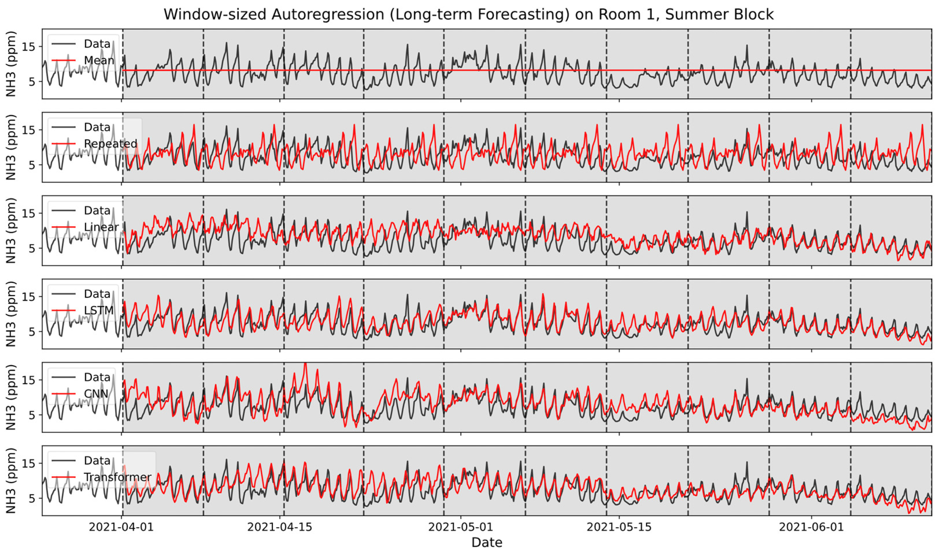
3.1. Sample Forecasting Plots

Figure 8 shows the model prediction results for two sample windows of iw = 84 (one week) and ow = 168 (two weeks) from Room 1 (when used as a test set), where each column represents one sample window from the summer and winter blocks, respectively, and each row corresponds to one of the six models tested (three baseline models and three neural network models). Note that the models used the ground-true values of the eight features (four original + four sin/cos temporal features; not shown in the figure except for the NH₃ concentration) as input and predicted all eight features in the output window (only the NH₃ concentration is shown in the gray area of the figure). The MAE of the sample was calculated using NH₃ concentration alone. Qualitative observations indicate that neural network models exhibit a superior performance compared with that of the simple baseline models. The neural network models captured periodic fluctuations and general trends in time series, whereas the baseline models failed. The LSTM model showed rather strong temporal oscillatory patterns, while the CNN model had a tendency of “smoothing” the temporal changes. The transformer model exhibited intermediate patterns between those of the two models. These characteristics arise from the different encoding strategies of the models.

Figure 9 shows a sample of long-term forecasting for 10 $\times$ iw time steps (10 weeks) with window-sized autoregression (See Section 2.3.5). The same models trained with window lengths of iw = 84 (1 week)/ow = 168 (2 weeks) were used to generate the forecasting plots. Note that only the initial input window of length iw (white background block on the leftmost side) was provided to the model, while the remaining data were hidden. Nevertheless, the neural network models managed to predict the long horizon reasonably well, even though the signal variability decreased abruptly after mid-May. With window-sized autoregression, the models can predict the arbitrarily long future, and we evaluated the model performance for the entire summer and winter blocks of each room (see the next section for the quantitative results).

3.2. Performance Metrics

We calculated and averaged the MAEs from the output windows (Window-MAE, or “W-MAE”) of the test sets in the cross-validation (Section 2.3.4), and from the long-term forecasting (Long-MAE, or “L-MAE”) with window-sized autoregression (Section 2.3.5) on the summer and the winter blocks of the three rooms.

Table 3. Mean absolute error (MAE). W-MAE was obtained from the output windows of size ow and L-MAE was obtained from the summer and the winter blocks with window-sized autoregression. All performance metrics were calculated for the test set in the three-fold cross-validation and the results were averaged to give the values presented in the table. The value of the best-performing model for each condition (iw & ow combination) is shown in bold. Note that iw and ow are expressed in the unit of week (“w”).

	iw = 1 w, ow = 1 w		iw = 1 w, ow = 2 w		iw = 1 w, ow = 3 w		iw = 1 w, ow = 4 w
	W-MAE	L-MAE	W-MAE	L-MAE	W-MAE	L-MAE	W-MAE	L-MAE
Mean	2.20	4.56	2.33	4.56	2.43	4.52	2.54	4.26
Repeat	2.47	4.90	2.71	4.90	2.85	4.82	2.98	4.58
Linear	2.15	2.59	2.24	2.55	2.20	2.34	2.15	2.42
LSTM	1.83	2.13	1.78	1.95	1.87	1.90	1.79	1.96
CNN	2.02	2.09	1.92	2.12	1.89	1.98	1.87	2.09
Transformer	1.89	1.87	1.90	2.07	1.87	1.97	1.73	1.83

summarizes the mean MAEs across the three rooms, and Figure 10 shows the results. Given one week of input, LSTM showed the minimum W-MAE of 1.83, 1.78, and 1.87 ppm for the prediction of one, two, and three weeks, respectively, whereas Transformer performed best with a W-MAE of 1.73 ppm for four-week prediction. In long-term estimation of spanning months, LSTM showed the minimum L-MAEs of 1.95 and 1.90 ppm when trained on predicting two and three weeks of windows. At the same condition, Transformer gave the minimum L-MAEs of 1.87 and 1.83 when trained on predicting one and four weeks of windows. Overall, the neural network models (LSTM, CNN, and Transformer) performed better than the baseline models (mean, repeat, and linear) across all conditions for both the W-MAE and L-MAE metrics. The linear baseline model showed an intermediate performance between the neural networks and the trainless baselines (mean and repeat). The performance gap between the baseline models and neural network models further increased in the L-MAE (Figure 10). The ratio of L-MAE over W-MAE, which estimates the relative error of long-term forecasting against short-term window forecasting (larger is worse), was 1.89 and 1.76 for the mean and the repeat baselines, respectively. For the linear, LSTM, CNN, and Transformer models, the ratios were 1.13, 1.09, 1.08, and 1.05, respectively. These small ratios, close to 1, indicate that the neural network models could perform long-term forecasting over a horizon far beyond the relatively short periods on which they were trained (1 to 4 weeks). Among the three neural network models tested with their specific configurations, the LSTM models usually performed the best for short-term forecasting (W-MAE), and the Transformer models performed well for long-term forecasting (L-MAE). However, the differences among the neural network models were small compared with the baseline models. In addition, Taylor diagrams that compare the models with three metrics—standard deviation, correlation coefficient, and centered root-mean-squared difference (RMSD)—show that LSTM, CNN, and Transformer present performances comparable to each other’s in terms of these metrics (See Figure S7 of Supplementary Materials) [57,58].

Figure 11 compares model performance with different input window lengths in the range of 2 ≤ iw ≤ 7 days. For each iw, the output range ow varied from 7 to 28 days (by one-day increments), and the MAEs were averaged over these output ranges. Both the W-MAE and L-MAE results showed that the neural network models had very little performance dependence on the input window length, indicating that even a short-length input of two days was sufficient for long-term (scale of months, measured by L-MAE) forecasting. However, the linear model performed worse with shorter-length inputs, and the overall errors were larger than those of the neural network models for all input length ranges tested. The trainless baseline models (mean and repeat) were not tested here because they were not trained on the input data and, thus, they did not have input-length dependency by design.

4. Discussion

Across all types of models used in the analysis, we selected regression or “one-shot” prediction that predicts all time points at once instead of iterative sequence prediction that predicts each time point one by one, recursively. One of the reasons for this choice was better stability in the training process because this method does not depend on previous predictions when predicting the next value, as opposed to the more traditional recursive sequence prediction [36,37]. This advantage is particularly important for long sequence prediction because small errors in early sequence prediction can accumulate and result in an unstable performance in the latter part of the sequence if recursive prediction is applied. However, a mere regression between the input and output sequences cannot encode the temporal interdependency among different time points in the input sequence because of the independency assumption of the regression, as can be observed in the linear model.

To encode this temporal dependency in the input sequence, we adopted the architectures of the following three representative neural networks: LSTM, CNN, and Transformer. These neural network models capture temporal information from the input sequence in their own designed manner (i.e., relational inductive bias [59]) and project the encoded representation onto the output sequence to make a prediction. The LSTM encoder updates the hidden states after each iteration in the input sequence to track temporal changes. The CNN encoder uses one-dimensional convolution along the temporal dimension to recognize local temporal patterns. The Transformer encoder applies multiheaded self-attention [48] to the input sequence to discover temporal dependency across all pairs of input time points. Regardless of the specific encoding schemes, all these neural network models showed a superior performance compared to that of the linear regression model, which did not assume any interdependency inside the input sequence. Performance differences among the three neural network models were minute compared with the gap between the linear and baseline models.

Therefore, we claim that the regression of the output variable (NH₃ concentration) from the input features and temporal encoding of the input sequence is crucial for stable and efficient forecasting. A disadvantage of window-based regression forecasting is that it can only predict fixed output lengths. We overcome this limitation by applying window-sized autoregression (WSAR). Unlike traditional point-wise autoregression, window-sized autoregression predicts the window length output simultaneously. Therefore, it does not suffer from unstable performance fluctuations and enables arbitrary long-range (multiples of the output length) forecasting. However, this approach must have the ground-true values of the initial input sequence when first applied to a certain data block. Therefore, estimating the length of the input required for a reliable prediction is important. Our additional analysis results in Figure 11 show that as short a time period as two days of input (equal to 24 time points) was sufficient for the neural network models to yield mid-to-long-term prediction on a scale of weeks to months. Thus, while CNN performance was quite close, LSTM and Transformers were the best models for short- and long-term predictions overall. We believe that the temporal encoding nature of all inputs, not just local patterns as CNN does, of LSTM and Transformer encoders provided them with the better prediction performance.

These findings have profound implications for designing future national NH₃ inventory projects. Currently, in many nations, measurements taken from a limited selection of farms are frequently deemed representative of the overall NH₃ emissions of the country; however, this practice is driven by constraints on measurement device ownership and the scarcity of appropriate research spaces. However, implementation of deep learning models, such as LSTM, CNN, and Transformer, allows the generation of highly accurate predictions using a minimal number of measurements, independent of the size of the facilities or environmental conditions. By increasing the sample size, we can obtain a more precise estimation of the NH₃ emissions from livestock farming, which closely mirror the actual quantities. Accurate quantification of NH₃ emissions can substantially improve the predictive accuracy of air quality indices, such as PM_2.5, in populated areas. Honing of predictions to minute-by-minute precision can facilitate proactive strategies to reduce odorous substances in response to predicted surges in NH₃ concentration. Furthermore, neural network models are indispensable for the real-time prediction and management of health conditions in livestock, including the animals, on farms. These models can rapidly detect changes in farm environments, equipping livestock farmers with crucial insights to guide the necessary interventions.

In the future, we plan to scale up experiment to a larger number of farms with more livestock species such as cows and chickens. With a larger scale of data available and combined with various environmental factors, we hope to advance the neural network models by training and testing on more challenging yet diverse data, perusing to their limits to be able to apply for various real-world scenarios.

5. Conclusions

Overall, we predicted NH₃ concentrations using various models and data collected from sow farms. Parameters such as temperature, humidity, ventilation rate, and NH₃ concentration were gathered, and a comparative evaluation of the baseline, linear regression, LSTM, CNN, and Transformer models was performed across three pig houses under identical environmental conditions. Consequently, the LSTM, CNN, and Transformer models demonstrated superior performance relative to that of the other models, with negligible differences between them. Further analysis, performed to consider the minimum number of required measurements, indicates that the input from two days is sufficient for medium-to-long-term predictions over several weeks. Neural network models enable real-time feedback, rapid responses, and automation, enhancing efficiency in monitoring and problem detection. Specifically, by extracting important features from time-series data, neural network models are more easily generalizable to a novel, unseen environment. Nevertheless, potential drawbacks exist. If the model lacks adequate support from environmental engineering for emission characteristics, it can become complex, requiring significant manpower and resources for maintenance. Furthermore, the acquisition of a substantial quantity of high-quality data remains a prerequisite for achieving the desired level of model reliability. However, addressing these shortcomings in long-term prediction can lead to various environmental and policy advantages, such as accurately measuring national NH₃ emissions in the future, establishing strategies for air pollutants generated by NH₃, and reducing odor in livestock farms. Additionally, if these techniques are integrated into real-time measurement devices, the device lifespan can be extended, thereby providing a significant cost advantage to farm owners.

References

1. Querol, X.; Alastuey, A.; Ruiz, C.R.; Artiñano, B.; Hansson, H.C.; Harrison, R.M.; Buringh, E.; Ten Brink, H.M.; Lutz, M.; Bruckmann, P.; et al. Speciation and Origin of PM10 and PM2.5 in Selected European Cities. Atmos. Environ. 2004, 38, 6547–6555. [Google Scholar] [CrossRef]
2. Feng, Y.; Penner, J.E. Global Modeling of Nitrate and Ammonium: Interaction of Aerosols and Tropospheric Chemistry. J. Geophys. Res. Atmos. 2007, 112, 1–24. [Google Scholar] [CrossRef]
3. Pinder, R.W.; Adams, P.J.; Pandis, S.N. Ammonia Emission Controls as a Cost-Effective Strategy for Reducing Atmospheric Particulate Matter in the Eastern United States. Environ. Sci. Technol. 2007, 41, 380–386. [Google Scholar] [CrossRef] [PubMed] [Green Version]
4. Tsimpidi, A.P.; Karydis, V.A.; Pandis, S.N. Response of Inorganic Fine Particulate Matter to Emission Changes of Sulfur Dioxide and Ammonia: The Eastern United States as a Case Study. J. Air Waste Manage. Assoc. 2007, 57, 1489–1498. [Google Scholar] [CrossRef]
5. Yang, F.; Tan, J.; Zhao, Q.; Du, Z.; He, K.; Ma, Y.; Duan, F.; Chen, G.; Zhao, Q. Characteristics of PM2.5 Speciation in Representative Megacities and across China. Atmos. Chem. Phys. 2011, 11, 5207–5219. [Google Scholar] [CrossRef] [Green Version]
6. Wang, Y.; Zhang, Q.Q.; He, K.; Zhang, Q.; Chai, L. Sulfate-Nitrate-Ammonium Aerosols over China: Response to 2000–2015 Emission Changes of Sulfur Dioxide, Nitrogen Oxides, and Ammonia. Atmos. Chem. Phys. 2013, 13, 2635–2652. [Google Scholar] [CrossRef] [Green Version]
7. Adams, R.M.; Hamilton, S.A.; Mccarl, B.A. The Benefits of Pollution Control: The Case of Ozone and U.S. Agriculture. Am. J. Agric. Econ. 1986, 68, 886–893. [Google Scholar] [CrossRef]
8. Tsai, Y.I.; Cheng, M.T. Visibility and Aerosol Chemical Compositions near the Coastal Area in Central Taiwan. Sci. Total Environ. 1999, 231, 37–51. [Google Scholar] [CrossRef]
9. Yuan, C.S.; Lee, C.G.; Liu, S.H.; Chang, J.C.; Yuan, C.; Yang, H.Y. Correlation of Atmospheric Visibility with Chemical Composition of Kaohsiung Aerosols. Atmos. Res. 2006, 82, 663–679. [Google Scholar] [CrossRef]
10. Wang, G.; Zhao, J.; Jiang, R.; Song, W. Rat Lung Response to Ozone and Fine Particulate Matter (PM2.5) Exposures. Environ. Toxicol. 2015, 30, 343–356. [Google Scholar] [CrossRef]
11. Lacressonnière, G.; Foret, G.; Beekmann, M.; Siour, G.; Engardt, M.; Gauss, M.; Watson, L.; Andersson, C.; Colette, A.; Josse, B.; et al. Impacts of Regional Climate Change on Air Quality Projections and Associated Uncertainties. Clim. Chang. 2016, 136, 309–324. [Google Scholar] [CrossRef]
12. Zhou, L.; Chen, X.; Tian, X. The Impact of Fine Particulate Matter (PM2.5) on China’s Agricultural Production from 2001 to 2010. J. Clean. Prod. 2018, 178, 133–141. [Google Scholar] [CrossRef]
13. Zou, J.; Liu, Z.; Hu, B.; Huang, X.; Wen, T.; Ji, D.; Liu, J.; Yang, Y.; Yao, Q.; Wang, Y. Aerosol Chemical Compositions in the North China Plain and the Impact on the Visibility in Beijing and Tianjin. Atmos. Res. 2018, 201, 235–246. [Google Scholar] [CrossRef]
14. Bhattarai, G.; Lee, J.B.; Kim, M.H.; Ham, S.; So, H.S.; Oh, S.; Sim, H.J.; Lee, J.C.; Song, M.; Kook, S.H. Maternal Exposure to Fine Particulate Matter during Pregnancy Induces Progressive Senescence of Hematopoietic Stem Cells under Preferential Impairment of the Bone Marrow Microenvironment and Aids Development of Myeloproliferative Disease. Leukemia 2020, 34, 1481–1484. [Google Scholar] [CrossRef] [Green Version]
15. Dianwu, Z.; Anpu, W. Estimation of Anthropogenic Ammonia Emissions in Asia. Atmos. Environ. 1994, 28, 689–694. [Google Scholar] [CrossRef]
16. Bouwman, A.F.; Lee, D.S.; Asman, W.A.H.; Dentener, F.J.; Van Der Hoek, K.W.; Olivier, J.G.J. A Global High-Resolution Emission Inventory for Ammonia. Glob. Biogeochem Cycles 1997, 11, 561–587. [Google Scholar] [CrossRef]
17. Streets, D.G.; Bond, T.C.; Carmichael, G.R.; Fernandes, S.D.; Fu, Q.; He, D.; Klimont, Z.; Nelson, S.M.; Tsai, N.Y.; Wang, M.Q.; et al. An Inventory of Gaseous and Primary Aerosol Emissions in Asia in the Year 2000. J. Geophys. Res. Atmos. 2003, 108. [Google Scholar] [CrossRef]
18. Huang, X.; Song, Y.; Li, M.; Li, J.; Huo, Q.; Cai, X.; Zhu, T.; Hu, M.; Zhang, H. A High-Resolution Ammonia Emission Inventory in China. Glob. Biogeochem Cycles 2012, 26, 1–14. [Google Scholar] [CrossRef]
19. Kang, Y.; Liu, M.; Song, Y.; Huang, X.; Yao, H.; Cai, X.; Zhang, H.; Kang, L.; Liu, X.; Yan, X.; et al. High-Resolution Ammonia Emissions Inventories in China from 1980 to 2012. Atmos. Chem. Phys. 2016, 16, 2043–2058. [Google Scholar] [CrossRef] [Green Version]
20. Misselbrook, T.H.; Gilhespy, S.L. Inventory of Ammonia Emissions from UK Agriculture 2017 DEFRA Contract SCF0107 Inventory Submission Report; Rothamsted Research: North Wyke, UK, 2019. [Google Scholar]
21. Tang, Y.S.; Braban, C.F.; Dragosits, U.; Dore, A.J.; Simmons, I.; Van Dijk, N.; Poskitt, J.; Dos Santos Pereira, G.; Keenan, P.O.; Conolly, C.; et al. Drivers for Spatial, Temporal and Long-Term Trends in Atmospheric Ammonia and Ammonium in the UK. Atmos. Chem. Phys. 2018, 18, 705–733. [Google Scholar] [CrossRef] [Green Version]
22. Maraveas, C. Durability Issues and Corrosion of Structural Materials and Systems in Farm Environment. Appl. Sci. 2020, 10, 990. [Google Scholar] [CrossRef] [Green Version]
23. Jeerh, G.; Zhang, M.; Tao, S. Recent Progress in Ammonia Fuel Cells and Their Potential Applications. J. Mater. Chem. A Mater. 2021, 9, 727–752. [Google Scholar] [CrossRef]
24. Verification of Environmental Technologies for Agricultural Production (VERA). Livestock Housing and Management Systems; International VERA Secretariat: Delft, The Nederland, 2018. [Google Scholar]
25. Schrade, S.; Zeyer, K.; Gygax, L.; Emmenegger, L.; Hartung, E.; Keck, M. Ammonia Emissions and Emission Factors of Naturally Ventilated Dairy Housing with Solid Floors and an Outdoor Exercise Area in Switzerland. Atmos. Environ. 2012, 47, 183–194. [Google Scholar] [CrossRef]
26. Philippe, F.X.; Laitat, M.; Wavreille, J.; Bartiaux-Thill, N.; Nicks, B.; Cabaraux, J.F. Ammonia and Greenhouse Gas Emission from Group-Housed Gestating Sows Depends on Floor Type. Agric. Ecosyst. Environ. 2011, 140, 498–505. [Google Scholar] [CrossRef]
27. Philippe, F.X.; Canart, B.; Laitat, M.; Wavreille, J.; Bartiaux-Thill, N.; Nicks, B.; Cabaraux, J.F. Effects of Available Surface on Gaseous Emissions from Group-Housed Gestating Sows Kept on Deep Litter. Animal 2010, 4, 1716–1724. [Google Scholar] [CrossRef] [Green Version]
28. Blunden, J.; Aneja, V.P.; Westerman, P.W. Measurement and Analysis of Ammonia and Hydrogen Sulfide Emissions from a Mechanically Ventilated Swine Confinement Building in North Carolina. Atmos. Environ. 2008, 42, 3315–3331. [Google Scholar] [CrossRef]
29. Sun, G.; Guo, H.; Peterson, J.; Predicala, B.; Laguë, C. Diurnal Odor, Ammonia, Hydrogen Sulfide, and Carbon Dioxide Emission Profiles of Confined Swine Grower/Finisher Rooms. J. Air Waste Manag. Assoc. 2008, 58, 1434–1448. [Google Scholar] [CrossRef] [PubMed]
30. Jo, G.; Ha, T.; Jang, Y.; Hwang, O.; Seo, S.; Woo, S.E.; Lee, S.; Kim, D.; Jung, M. Ammonia Emission Characteristics of a Mechanically Ventilated Swine Finishing Facility in Korea. Atmosphere 2020, 11, 1088. [Google Scholar] [CrossRef]
31. Saha, C.K.; Ammon, C.; Berg, W.; Fiedler, M.; Loebsin, C.; Sanftleben, P.; Brunsch, R.; Amon, T. Seasonal and Diel Variations of Ammonia and Methane Emissions from a Naturally Ventilated Dairy Building and the Associated Factors Influencing Emissions. Sci. Total Environ. 2014, 468–469, 53–62. [Google Scholar] [CrossRef] [PubMed]
32. Hempel, S.; Saha, C.K.; Fiedler, M.; Berg, W.; Hansen, C.; Amon, B.; Amon, T. Non-Linear Temperature Dependency of Ammonia and Methane Emissions from a Naturally Ventilated Dairy Barn. Biosyst. Eng. 2016, 145, 10–21. [Google Scholar] [CrossRef] [Green Version]
33. Hempel, S.; Adolphs, J.; Landwehr, N.; Janke, D.; Amon, T. How the Selection of Training Data and Modeling Approach Affects the Estimation of Ammonia Emissions from a Naturally Ventilated Dairy Barn-Classical Statistics versus Machine Learning. Sustainability 2020, 12, 1030. [Google Scholar] [CrossRef] [Green Version]
34. Feng, K.; Wang, Y.; Hu, R.; Xiang, R. Continuous Measurement of Ammonia at an Intensive Pig Farm in Wuhan, China. Atmosphere 2022, 13, 442. [Google Scholar] [CrossRef]
35. Lara-Benítez, P.; Carranza-García, M.; Riquelme, J.C. An Experimental Review on Deep Learning Architectures for Time Series Forecasting. Int. J. Neural Syst. 2021, 31, 2130001. [Google Scholar] [CrossRef]
36. Lim, B.; Zohren, S. Time-Series Forecasting with Deep Learning: A Survey. Philos. Trans. R. Soc. A Math. Phys. Eng. Sci. 2021, 379, 20200209. [Google Scholar] [CrossRef]
37. Benidis, K.; Rangapuram, S.S.; Flunkert, V.; Wang, Y.; Maddix, D.; Turkmen, C.; Gasthaus, J.; Bohlke-Schneider, M.; Salinas, D.; Stella, L.; et al. Deep Learning for Time Series Forecasting: Tutorial and Literature Survey. ACM Comput. Surv. 2022, 55, 1–36. [Google Scholar] [CrossRef]
38. Kim, S.J.; Lee, M.H. Design and Implementation of a Malfunction Detection System for Livestock Ventilation Devices in Smart Poultry Farms. Agriculture 2022, 12, 2150. [Google Scholar] [CrossRef]
39. Kim, J.G.; Lee, S.Y.; Lee, I.B. The Development of an LSTM Model to Predict Time Series Missing Data of Air Temperature inside Fattening Pig Houses. Agriculture 2023, 13, 795. [Google Scholar] [CrossRef]
40. Sheng, S.; Lin, K.; Zhou, Y.; Chen, H.; Luo, Y.; Guo, S.; Xu, C.Y. Exploring a Multi-Output Temporal Convolutional Network Driven Encoder-Decoder Framework for Ammonia Nitrogen Forecasting. J. Environ. Manag. 2023, 342, 118232. [Google Scholar] [CrossRef]
41. Lecun, Y.; Bengio, Y.; Hinton, G. Deep Learning. Nature 2015, 521, 436–444. [Google Scholar] [CrossRef] [PubMed]
42. Peng, S.; Zhu, J.; Liu, Z.; Hu, B.; Wang, M.; Pu, S. Prediction of Ammonia Concentration in a Pig House Based on Machine Learning Models and Environmental Parameters. Animals 2023, 13, 165. [Google Scholar] [CrossRef] [PubMed]
43. Wang, K.; Liu, C.; Duan, Q. Piggery Ammonia Concentration Prediction Method Based on CNN-GRU. In Journal of Physics: Conference Series; IOP Publishing Ltd.: Bristol, UK, 2020; Volume 1624. [Google Scholar]
44. Bengio, Y.; Courville, A.; Vincent, P. Representation Learning: A Review and New Perspectives. IEEE Trans. Pattern Anal. Mach. Intell. 2013, 35, 1798–1828. [Google Scholar] [CrossRef] [Green Version]
45. Hochreiter, S.; Schmidhuber, J. Long Short-Term Memory. Neural. Comput. 1997, 9, 1735–1780. [Google Scholar] [CrossRef]
46. Chung, J.; Gulcehre, C.; Cho, K.; Bengio, Y. Empirical Evaluation of Gated Recurrent Neural Networks on Sequence Modeling. NIPS 2014 Workshop on Deep Learning; NeurIPS: Lake Tahoe, NV, USA, 2012. [Google Scholar]
47. Krizhevsky, A.; Sutskever, I.; Hinton, G.E. ImageNet Classification with Deep Convolutional Neural Networks. Advances in Neural Information Processing Systems 25; NeurIPS: Montreal, CA, 2014. [Google Scholar]
48. Vaswani, A.; Shazeer, N.; Parmar, N.; Uszkoreit, J.; Jones, L.; Gomez, A.N.; Kaiser, L.; Polosukhin, I. Attention Is All You Need. Adv. Neural Inf. Process. Syst. 2017, 30, 6000–6010. [Google Scholar]
49. Bai, S.; Kolter, J.Z.; Koltun, V. An Empirical Evaluation of Generic Convolutional and Recurrent Networks for Sequence Modeling. arXiv 2018, arXiv:1803.01271. [Google Scholar]
50. Li, S.; Jin, X.; Xuan, Y.; Zhou, X.; Chen, W.; Wang, Y.-X.; Yan, X. Enhancing the Locality and Breaking the Memory Bottleneck of Transformer on Time Series Forecasting. Adv. Neural Inf. Process. Syst. 2019, 32, 5243–5253. [Google Scholar]
51. Fan, C.; Zhang, Y.; Pan, Y.; Li, X.; Zhang, C.; Yuan, R.; Wu, D.; Wang, W.; Pei, J.; Huang, H. Multi-Horizon Time Series Forecasting with Temporal Attention Learning. In Proceedings of the ACM SIGKDD International Conference on Knowledge Discovery and Data Mining, Anchorage, AK, USA, 4–8 August 2019; Association for Computing Machinery: New York, NY, USA, 2019; pp. 2527–2535. [Google Scholar]
52. Park, S.; Jung, M.W.; Seo, S.; Woo, S.E.; Hwang, O.; Halder, J.N.; Jang, Y.; Jo, G.; Park, J. Comparison of Ammonia Emission Characteristics from Sows in Summer and Winter. J. Korean Soc. Atmos. Environ. 2022, 38, 895–905. [Google Scholar] [CrossRef]
53. Fundamentals, I.-P. American Society of Heating, Refrigerating and Air-Conditioning Engineers (ASHRAE). ASHRAE Handbook; ASHRAE: Atlanta, GA, USA, 1993. [Google Scholar]
54. Sonntag, D. Important New Values of the Physical Constants of 1986, Vapour Pressure Formulations Based on the ITS-90, and Psychrometer Formulae. Zeitschrift für Meteorologie 1990, 40, 340–344. [Google Scholar]
55. Kiranyaz, S.; Avci, O.; Abdeljaber, O.; Ince, T.; Gabbouj, M.; Inman, D.J. 1D Convolutional Neural Networks and Applications: A Survey. Mech. Syst. Signal Process. 2021, 151, 107398. [Google Scholar] [CrossRef]
56. Loshchilov, I.; Hutter, F. Decoupled Weight Decay Regularization. arXiv 2017, arXiv:1711.05101. [Google Scholar]
57. Taylor, K.E. Summarizing Multiple Aspects of Model Performance in a Single Diagram. J. Geophys. Res. Atmos. 2001, 106, 7183–7192. [Google Scholar] [CrossRef]
58. Peter, A. Rochford SkillMetrics: A Python Package for Calculating the Skill of Model Predictions against Observations 2016. Available online: http://github.com/PeterRochford/SkillMetrics (accessed on 17 July 2023).
59. Battaglia, P.W.; Hamrick, J.B.; Bapst, V.; Sanchez-Gonzalez, A.; Zambaldi, V.; Malinowski, M.; Tacchetti, A.; Raposo, D.; Santoro, A.; Faulkner, R.; et al. Relational Inductive Biases, Deep Learning, and Graph Networks. arXiv 2018, arXiv:1806.01261. [Google Scholar]
Figure 1. (a) Top-view and (b) cross-section of the pig house, illustrating the sequence of NH3 measurements in this study. The NH3 inlet concentration was sampled and analyzed from the mid-ceiling area of the pigsty.
Atmosphere 14 01248 g001
Figure 2. Pipeline of data analysis. Raw data are preprocessed with scaling, feature addition, and temporal segmentation to data blocks. Then, each data block is sliced with sliding windows. Widows of input and output data from different rooms are assigned one of training, validation, and test set for cross-validation. Finally, test results are evaluated with metrics W-MAE and L-MAE (See Section 2.3.5 for definition of the metrics).
Atmosphere 14 01248 g002
Figure 3. The averaged NH3 concentration in the summer block (left) and the winter block (right) of the three rooms. The red area denotes the duration of device maintenance and restoration.
Atmosphere 14 01248 g003
Figure 4. Illustration of applying the sliding window technique with an input length iw, an output length ow, and a stride.
Atmosphere 14 01248 g004
Figure 5. Architecture of the four types of neural network models used for forecasting. All models flatten the data before being connected to the final dense layer. Neurons in the final dense layer represent the prediction values at each time point in the output window. (A) Linear regression. Input and output neurons are densely and independently connected, treating each time and feature independently. (B) Long Short-Term Memory (LSTM) regression. Hidden units are updated from both the current input and the past hidden state, giving them the ability to encode temporal information. (C) Convolutional Neural Network (CNN) regression. The 1D convolution kernel moves along the temporal dimension, encoding local (short-term) temporal patterns. (D) Transformer regression. Temporal encoding and self-attention encode mutual dependency among input values.
Atmosphere 14 01248 g005
Figure 6. Cross-validation across the three rooms. Each room was assigned as one of the training, validation, and test sets. The performance metrics from the test sets were averaged to provide the overall performance evaluation of a model.
Atmosphere 14 01248 g006
Figure 7. Window-sized autoregression. After initial prediction from the ground-true input of length iw, the model takes the last iw prediction values as a new input and predicts the same length output.
Atmosphere 14 01248 g007
Figure 8. Forecasting plots for two sample windows, one (left column) from the 61st window in the summer block and the other (right column) from the 61st window in the winter block of Room 1, respectively. Each row shows the prediction of one of the six models tested (the three baseline models and three neural network models). The black line in the white background indicates NH3 concentration in the input window. The black and red lines in the gray background indicate the ground-true value and the model prediction of NH3 concentration, respectively, in the output window. MAE (mean absolute error) was calculated within each output window (gray background).
Atmosphere 14 01248 g008
Figure 9. Long-term forecasting plots for the summer block of Room 1. Models received the input of length iw (the leftmost block with the white background) and predicted for the remaining parts (the gray background). The plot was cut at the length of 10 × iw time steps (=840, equal to 10 weeks) in the output for visualization purposes, but the models actually predicted for the entire summer and winter blocks. The dashed vertical lines separate the length of iw.
Atmosphere 14 01248 g009
Figure 10. Model performance comparison. All metrics were measured and averaged across the test sets in the 3-fold cross-validation. LSTM, Long Short-Term Memory; CNN, Convolutional Neural Network.
Atmosphere 14 01248 g010
Figure 11. Dependence of the mean average error (MAE) on the input window length (iw). Circles represent the mean MAE over the range of different output lengths ow given iw. Error bars indicate standard deviation.
Atmosphere 14 01248 g011