Abstract
By using Weather Research and Forecasting Model (WRF) to simulate a southwest vortex precipitation process, this work studies the correlations between entrainment rate (λ) and dynamical parameters in the cloud and further fit λ. We relate the probability density distribution (PDF) to the parameterization of λ and find that the greater the probability, the larger the slope of the logarithmic liner function. The slope of the log-linear fitting function in fitting decreases for developing and enhancing cumulus clouds, which is related to the increase in updraft motion and the decrease in λ. Then, we group clouds according to cloud top heights and calculate average λ and dynamic parameters, and the results indicate that when only one dynamic parameter is used, vertical wind velocity (w) is more suitable than buoyancy (B) to be used to fit λ. The fitting functions combing one single parameter and more parameters by principal components regression are compared with two traditional schemes, and we found that λ obtained by our fitting schemes are between the two traditional schemes. Because the principal component regression method takes into account the interaction between more dynamic factors and entrainment, the fitting function, including w and B, is suitable to be applied to fit λ in the parameterization scheme for cumulus clouds.
1. Introduction
Both cloud and climate can be significantly affected by entrainment [1,2,3,4,5,6]. The entrainment and mixing process impacts the simulation effect of weather and climate models [7,8,9,10]. So, it is important to import a reliable entrainment rate (λ) parameterization scheme into the model to improve the simulation effect.
Turner [11] assumed that the cross-section of the cloud was approximately circular and proposed that λ was inversely proportional to the cloud radius. This λ parameterization scheme formed the theoretical basis for many convective parameterization schemes, such as the climate model developed by the International Pacific Research Center of the University of Hawaii [1] and European Centre for Medium-Range Weather Forecasts (ECMWF) model [12]. But Siebesma and Cuijpers [13] found that the λ obtained using this scheme is much smaller than that obtained in the model. Some parameterization schemes further assumed that the change in the cloud effective radius (Re) is negligible, so λ can be regarded as a fixed value [14]. Some other schemes assumed that Re is proportional to the height of the cloud top [15] or that λ is inversely proportional to the height (z) in the cloud [16]. Some schemes proposed that λ depends on the distribution of relative humidity [17,18]. Some other studies associated λ with dynamic variables. For example, Neggers et al. [19] used a large-eddy simulation to simulate shallow cumulus clouds and proposed that λ is inversely proportional to vertical wind velocity (w). Gregory [20] considered buoyancy (B) in the cloud and proposed that λ is proportional to B/w2. Del Genio and Wu [21] found that the empirical parameters in the scheme of Neggers et al. [19] vary greatly with height in different clouds. In contrast, the scheme of Gregory [20] relatively accords with their results. In addition, von Salzen and McFarlane [22] suggested that λ is proportional to dB/dz. de Rooy and Siebesma [16] proposed that there is a correlation between λ and B/w2, w −1dw/dz. Lin [23] also related λ to B and proposed that λ is proportional to Bφ, where φ is a fitting empirical parameter.
Dawe and Austin [24] found the product of mean B and the change rate of environmental density potential temperature with a height that best fit λ and proposed that λ negatively correlates with the product. Zhang et al. [25] used the cloud-resolving model to fit λ and found that the relationship between λ and w−1 is in line with second-order polynomials. Their research shows that for clouds at different stages of development, both the cloud top height and the parameterization of λ are inconsistent. Lu et al. [26] related λ to the dissipation rate factor and used principal component regression to analyze the relationship between λ and some dynamic parameters. Romps and Kuang [27] proposed that entrainment is intrinsically random, so the parameterization of λ should also be a random process accompanied by discontinuous mixings in rising clouds. All in all, the existence of so many parameterization schemes indicates that there is still uncertainty as to which scheme best represents λ, so it is necessary to develop more parameterization schemes to test these hypotheses in different clouds and environmental conditions.
The above-investigated clouds mainly developed over the plain or ocean. Southwest vortex cumulus clouds are formed under the interaction between the particular topography of the Tibetan Plateau (Figure 1) and atmospheric circulation. The southwest monsoon airflow interacts with the topography and creates strong vertical shear. The combination of them leads to the occurrence of inclined vorticity and the rapid growth of vertical vorticity, resulting in the formation of the southwest vortex. So, the development mechanism and λ parameterization of the southwest vortex cumulus could deviate from the clouds that grow over the plain or ocean. Therefore, this study used Weather Research and Forecasting Model (WRF3.8) to simulate a southwest vortex precipitation case near Sichuan Basin, China, from 8 to 9 July 2010 (Beijing time, the same as below), then calculated λ. Based on the relationships between λ and physical quantities, the parameterization of λ was analyzed and compared with some previous classic schemes.
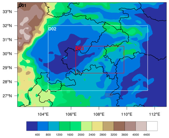
Figure 1.
Zone setting of WRF simulation, and d01, d02 and d03 (black, white and red rectangles) represent the second and the third nest, respectively. The abscissa and ordinate are longitude and latitude, respectively. The color bar refers to terrain height (unit: meter).
2. Simulation Scheme and Method
2.1. Simulation Scheme
In this study, a threefold nested mesh scheme (Figure 1) was used for simulation. The spin-up time period for model is 12 h. The horizontal resolutions were 16 km, 4 km, and 1 km, respectively. The vertical direction was divided into 65 layers, and the model top height was 50 hPa. Zhang et al. [25] used 1 km resolution to calculate λ, and they found that the results of 1 km resolution were similar to those of 100 m high resolution from large-eddy simulation. Therefore, λ was calculated using only 1 km resolution in threefold nested mesh in this study.
The microphysics scheme used the Lin scheme, which is a detailed microphysics scheme in WRF, and many scholars have used this scheme to simulate convective clouds [28]. The cumulus convective parameterization scheme of the first and second mesh used the Kain–Fritsch scheme, and some other WRF simulations also selected this scheme and simulated cumulus cloud well [29]. The third mesh was integrated into the model resolvable process without a convective parameterization scheme. The long-wave and short-wave radiation schemes selected for the model were RRTM and Dudhia, respectively. The near-formation scheme used revised MM5, and the land surface process scheme was Noah’s scheme. The planetary boundary layer scheme selected the YSU scheme. The output of d03 was performed every ten minutes to obtain more two-dimensional cumulus samples for fitting λ. The simulation started from 08:00 on 8 July to 14:00 on 9 July 2010. During this period, a typical southwest vortex strong precipitation process occurred.
The simulated and observed precipitation particle content was compared in Figure 2 to test the simulation effect. Because of the observation height limit of the Tropical Rainfall Measuring Mission (TRMM), precipitable water content (PWC) was only compared at the altitude from 3.8 to 18 km. The simulated PWC is close to that observed by TRMM, and the average difference within the height range between them is only 0.03 g/m3. In addition, both WRF and TRMM showed a decreasing trend with heights above 0.5 km. So WRF, with the above schemes, well simulated the vertical distribution of precipitation particles in this southwest vortex case.
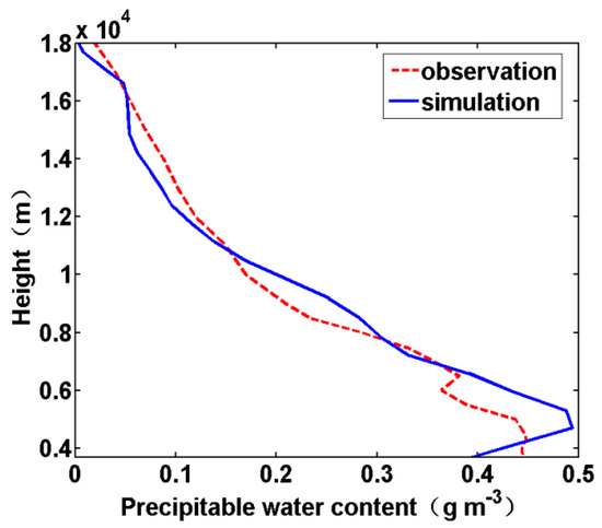
Figure 2.
Vertical profiles of precipitable water contents of WRF (blue solid line) and TRMM (red dashed line) at 0400 BST9 9 July 2010.
2.2. Method
Before calculating λ, clouds need to be identified in the model. Firstly, the simulated grid points with a cloud water mixing ratio more prominent than 0.05 g/kg were regarded as the points in the cloud. The grid points in the cloud along the latitude (or longitude) direction in a particular layer formed a one-dimensional grid point data set. A vertically continuous collection of one-dimensional points then formed a two-dimensional cloud along latitude (or longitude) direction. The maximum w and the average B in each two-dimensional cloud must, respectively, exceed 1 m/s and 0 m/s2 to ensure all identified clouds are growing clouds. Based on the maximal height of two-dimensional clouds, all identified clouds can be grouped by cloud top height. The traditional method [30] was used to calculate λ in this study.
3. Result
3.1. Fitting of λ Based on PDF
The joint probability density function (PDF) [24,31] was used to fit quantities in the cloud. The units for grouping physical quantities in PDF are 0.5 km−1 (λ), 0.5 m/s (w), and 0.5 m/s2 (B), respectively. Figure 3 shows PDF distributions of quantities and the relationship between λ and dynamic quantities, and the distributions of PDF here are similar to the results of Dawe and Austin [24]. λ is negatively correlated with the two dynamic factors, consistent with Lu et al.’s observation and simulation results [26]. The power law function was used to fit λ as follows:
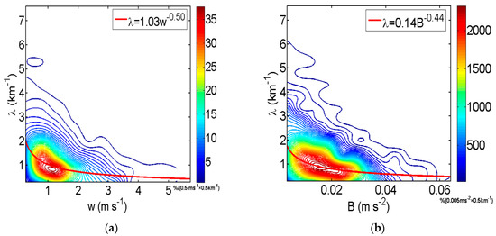
Figure 3.
Joint probability density function (PDF) of (a) entrainment rate (λ) vs. vertical velocity (w) and (b) λ vs. buoyancy (B) for all eligible clouds. The red lines denote the fitted power law functions.
The power law function in Equation (1) shows the linear relationship for the logarithm of quantities. Therefore, a and b are the intercept and the slope of the linear relationship, respectively. Moreover, b represents the change rate of λ with physical quantities. The obtained power law functions (the red curves in Figure 3) also confirm the negative correlations as follows:
The negative signs in −0.5 and −0.44 and the positive signs in 1.03 and 0.14 jointly lead to the negative correlations. The mechanism is that entrainment decreases B by reducing the temperature difference inside and outside the cloud, and vertical upward motion weakens. On the other hand, the enhancement of B and the upward motion mean lower exposure to clouds in the environment when rising a certain distance, so λ decreases. Both two equations include only one dynamic factor (w or B), so there are only two empirical parameters in the two equations.
But entrainment interacts with the two dynamic factors together [26]. Therefore, it is necessary to use the principal component regression method, which is a regression analysis with the principal component as the independent variable and is a method to analyze multivariate collinearity problems. The procedure is outlined as follows: (1) convert the independent variables into standardized variables; (2) determine the principal component of this standard variable; (3) use the least square method as a dependent variable to determine the regression of principal components; and (4) replace the principal components in the regression equation with linear combinations of standard variables to obtain the regression equation based on standard variables. Using the principal component regression method, entrainment was related to the two dynamic factors (Equation (4)). The fitted data in Equation (4) and Figure 3 are precisely identical.
In Equation (4), the positive and negative signs in coefficients also indicate the negative correlations between entrainment and physical factors. Furthermore, −0.31 and −0.27 can also be seen as the slopes of the linear relationships of logarithms or the change rates of λ with physical quantities. The larger absolute value (−0.31) for w means that compared with B, w contributes more to the variation in λ.
3.2. Variation in Fitting Parameters with PDF
The fitting functions for Figure 3 include λ in each layer of all identified cumulus clouds. When PDF is more significant than 30%/(0.5 m/s × 0.5 km−1) in Figure 3a, the calculated λ values are close to the red fitting curve. However, when PDF is smaller than 30%/(0.5 m/s × 0.5 km−1), the calculated λ values are far from the red fit curve. That is to say, the fitting values of Equations (3) and (4) only represent the λ values with high probability well.
Figure 4 compares the λ fitted according to Equations (3)–(5) with the calculated λ in the model. The range of fitted λ is smaller than that of calculated values. In addition, when the PDF is relatively large, the fitted λ is approximate to the calculated values. But for relatively small PDFs, the distributions of the fitted and computed values are somewhat dispersive. Therefore, the fitting function cannot represent all λ values in different probability ranges well. So, λ parameterization may be different for different PDFs. Dawe and Austin [24] used PDF to parameterize λ, but they did not further analyze the sensitivity of λ parameterization to different PDF ranges.
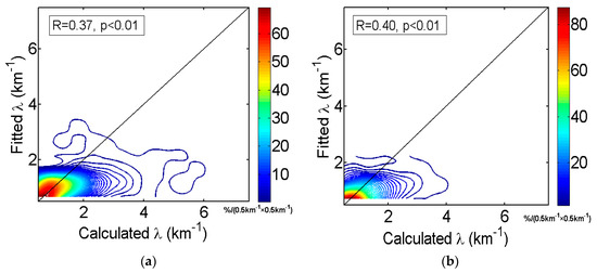
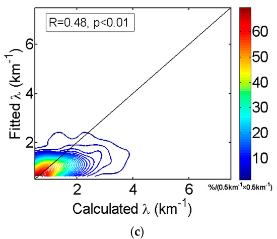
Figure 4.
Fitted entrainment rates (λ) expressed by (a) vertical velocity (w), (b) buoyancy (B), and (c) both w and B in Equations (2), (3), and (4), respectively, as a function of estimated λ in the form of PDF. The black lines denote 1:1 isolines. Each legend provides the correlation coefficient (R) and the p value of the correlation.
To analyze the sensibility of parameterization of λ to PDF, Figure 5 uses scatters to fit the relationship between dynamic parameters and λ in different PDF ranges. The logarithmic coordinates in Figure 5 can make the power law fit function linear, and the superscript numbers in Equations (2)–(4) are the slopes of a logarithmic linear function. Unlike Figure 3, the data in Figure 5 are grouped by logarithms of physical quantities. The black dots in Figure 5a represent all values, and the blue and red dots represent the values with PDF larger than 100%/(0.02 × 0.02) and 200%/(0.02 × 0.02), respectively. Similarly, the black dots in Figure 5b represent all values, and the blue and red dots represent the values with PDFs larger than 100%/(0.03 × 0.02) and 150%/(0.03 × 0.02), respectively. In Figure 5, 0.02 or 0.03 represents the interval for grouping logarithms of physical quantities. The result shows that with the increase in PDF, the slope of the log-linear function also gradually increases. In other words, the change rate of λ with dynamic parameter (w or B) is larger for the larger probability distribution of physical quantity.
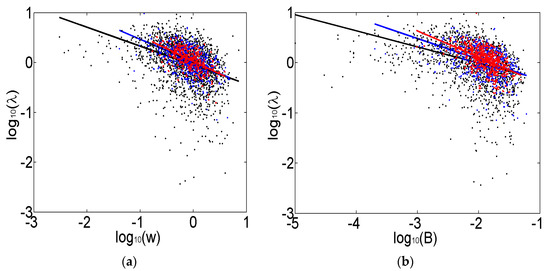
Figure 5.
Scatter plots of the relationships between entrainment rate and (a) vertical velocity (w), and (b) buoyancy (B) for different PDF ranges. The three straight lines with different colors denote the logarithmic linear fitting lines for different PDF ranges.
To discuss the trends in Figure 5 quantitatively, the slope changes of the log-linear function with PDF are analyzed in Figure 6, which shows that, regardless of using single or two dynamic parameters to fit λ (solid blue line and dashed blue line in Figure 6a), with the increase in PDF, the absolute value of slope change increases, which is consistent with the result in Figure 5a. However, as the PDF between λ and w increases, the absolute value of slope change (λ with B) decreases (solid red line and dotted red line in Figure 6a), which indicates that the PDF between λ and w does not correspond precisely to the PDF between λ and B. Similar results are shown in Figure 6b. In addition, when using a single dynamic variable (w or B), the slope absolute value of λ with the dynamic variable is larger than when two variables are used simultaneously. This is in line with theoretical expectations. For example, when only the relationship between λ and w is considered, the change rate of λ with w is necessarily greater than the change rate of λ with w when more quantities (e.g., B) are simultaneously considered, which is also shown in the slope parameter corresponding to w in Equations (2) and (4).
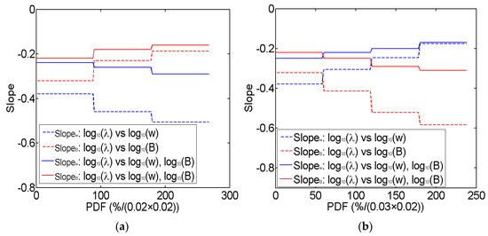
Figure 6.
Absolute slope changes of logarithmic linear fitting with the PDF between (a) entrainment rate (λ) and vertical velocity (w), (b) λ and buoyancy (B). The blue and red solid lines represent the changed slopes of λ with w (blue) and B (red), respectively, when a single dynamical variable is used to fit λ. The blue and red dashed lines represent the changed slopes of λ with w (blue) and B (red), respectively, when two dynamical variables are used to fit λ at the same time.
3.3. Variation in Fitting Parameters over Time
The above PDF-based analysis does not include the change in parameterization over time. But, in fact, as the cloud develops, the empirical parameters in λ parameterization also change. Figure 7 shows the fitting slope between λ and dynamic parameters as a function of time. The figure’s starting and ending times are when cumulus clusters were discovered and coalescence began. The slopes in Figure 7a,b are the slope of λ with w (blue line, slopew) and the slope of λ with B (red line, slopeB) when λ is fitted with a single dynamic parameter (w or B) and two dynamic parameters (w and B), respectively. The realized and dashed lines represent the PDF between the logarithms of λ and w greater than 100%/(0.02 × 0.02) and 200%/(0.02 × 0.02), respectively. Regardless of whether single or two dynamic parameters are used, and regardless of whether the PDF is greater than 100%/(0.02 × 0.02) or 200%/(0.02 × 0.02), the absolute value of slopew gradually decreases over time. The PDF between λ and w mentioned above does not correspond exactly to the PDF between λ and B, but the absolute value of slopeB also decreases over time. Figure 7c,d are similar to Figure 7a,b but based on the logarithm between λ and B. Similarly, the decreasing trend of the absolute value of slopeB is unrelated to PDF and the number of dynamic parameters for fitting. The absolute value of slopew also shows a decreasing trend over time.
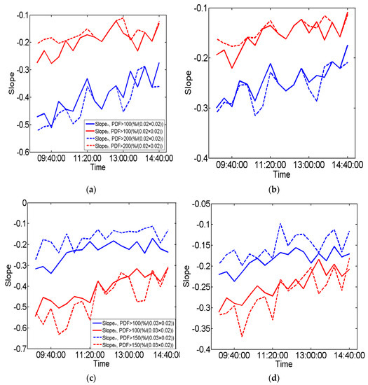
Figure 7.
Time series of slopes of logarithmic linear fitting, (a,b) represent the changed slopes of λ with w and B when a single dynamical variable and two dynamical variables, respectively, are used to fit λ. The solid and dashed lines in (a,b) represent the changes of slope for between logarithmic PDF between λ and w. (c,d) are similar to (a,b) but are based on logarithmic PDF between λ and B. See text for more details.
The slope changes in Figure 7 are closely related to the development of λ, w, and B during this period. Figure 8 shows that λ gradually decreases while w and B increase, indicating that the clouds are developing. This is the reason for the decreasing change rates of λ with w and B in Figure 7, leading to the change in fitting parameters. In view of the variation trends of w and B in Figure 8, it can be inferred that the change rates of λ with w or B may both decrease when cumulus clouds are developing and enhancing, which needs to be verified by more studies in the future. The above analysis shows uncertainties in λ fitting based on PDF, and the fitting parameters could change significantly when clouds are developing. Therefore, the parameterization of λ is a complex problem. In addition to the PDF range and the development of clouds, the parameterization of λ is also closely related to the type and height of the cloud. Therefore, we need to simplify λ parameterization, which will be discussed below.
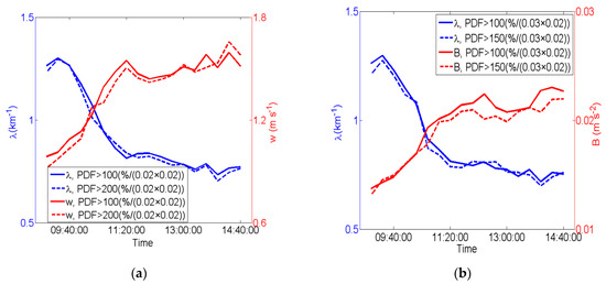
Figure 8.
Time series of domain-averaged entrainment rate (λ), vertical velocity (w) and buoyancy (B), (a,b) are based on the PDF between logarithmic λ and w and between logarithmic λ and B, respectively. The solid and dashed lines represent different PDF ranges. See text for more details.
3.4. Fitting of λ Based on Cloud-Averaging
Current large-scale climate models cannot identify individual cumulus clouds with their detailed features. So, we can classify the clouds within the development stage according to some characteristics so that the relationship between the λ and dynamic parameters based on cloud averaging can be obtained. Zhang et al. [25] classified clouds according to cloud top height in the model for different clouds. This section adopted a similar method to classify all qualified two-dimensional clouds according to the simulated cloud top height. The method for classifying clouds has been introduced in Section 2.2. Then, the average λ, w, and B in different altitudes were obtained for parameterization.
Figure 9a,b show the relationships between average λ and average dynamic parameters. Similar to Figure 3, significant negative correlations exist between the two dynamic factors and λ (the correlation coefficients in Figure 9a,b are −0.78 and −0.69, respectively). The negative correlation between λ and w is similar to the parameterization scheme of Neggers et al. [19]. The reasons can be explained from two perspectives: (1) The enhancement of λ inhibited the upward motions in clouds. The reason is that, compared to the air within the developing cumulus cloud, the entrained dryer and colder environmental air reduce the temperature in the cloud after mixing, thus reducing the temperature difference between the inside and outside clouds [31]. B is a physical quantity that measures this temperature difference, so an increase in entrainment will make B smaller. According to Newton’s second law of motion, the decrease in B will lead to the weakening of the upward motion (w) in the cloud. (2) When B and w increase, the upward motion in the cloud will enhance, and the time required for clouds to rise a certain distance in the vertical direction will be shortened, so the interaction between cloud and environment weakens [32]. This results in a decrease in λ. Therefore, entrainment and the physical quantities in the cloud affect interactively.
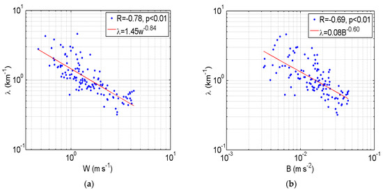
Figure 9.
Scatter plots of mean entrainment rate (λ) vs. (a) vertical velocity (w) and (b) buoyancy (B). Each legend provides the correlation coefficient (R) and p values for the correlation. The red lines denote the fitted power law functions.
According to the relationships in Figure 9, the two following equations for fitting λ were obtained:
Similar to Figure 4, the λ fitted according to Equations (5) and (6) are compared in Figure 10 with the values in the model. Figure 10 shows that the correlation coefficient for Equation (5) is 0.70, which is larger than the correlation coefficient (0.59) for Equation (6). This is similar to the simulation results of Lu et al. [26], which indicates that if only one dynamic parameter is used for fitting λ, w might be more suitable than B. Zhang et al. [25] only used w in their parameterization scheme without taking B into account. In addition, for the calculated λ less than 1.5 km−1, the correlation coefficient between the fitting and the calculated value is 0.80. However, for λ calculated greater than 1.5 km−1, the fitting values are significantly lower. Lu et al. [26] also found that the fitting value is smaller than the calculated value when λ is relatively large.
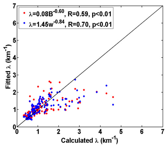
Figure 10.
Fitted entrainment rates (λ) from Equation (5) (blue points) and Equation (6) (red points) as a function of estimated λ. The black lines denote 1:1 isoline. The fitted function, correlation coefficient (R), and the p value of the correlation for each equation are provided, respectively, in the legend.
Equations (5) and (6) are compared with some traditional parameterization schemes to verify the fitting schemes. The red points in Figure 11 represent the following scheme (NS02) proposed by Neggers et al. [19]:
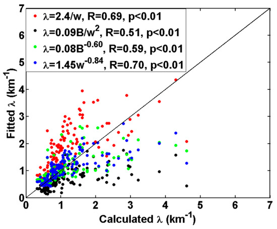
Figure 11.
Fitted entrainment rates (λ) from NS02 (red points), GR01 (black points), Equation (5) (blue points), and Equation (6) (green points) as a function of estimated λ. The black line denotes 1:1 isoline. The fitted function, correlation coefficient (R), and the p value of the correlation for each equation are provided, respectively, in the legend.
The empirical parameters in Equations (7) and (8) are recommended by Neggers et al. [19] and Gregory [20], respectively. Figure 11 shows that our fitted λ values are located between the values of NS02 and GR01. The fitted values of NS02 and GR01 are mainly located above and below the black 1:1 contour, respectively. That is to say, compared with our schemes in Figure 9, the two traditional schemes overestimate and underestimate λ, respectively. As mentioned above, for relatively small λ, Equation (5) underestimates λ, but the fitting value of GR01 is still significantly larger. For the correlation coefficient, the corresponding value of Equation (5) (0.70) is greater than that of NS02 and GR01 (0.69 and 0.51, respectively). Furthermore, the fitting values of Equation (6) are also between the fitting values of NS02 and GR01.
Equations (5) and (6) only include the relationship between one dynamic variable (w or B) and λ. But as mentioned above, entrainment interacts together with the two dynamic factors. Therefore, similar to Equation (4), according to the principal component regression method, three fitting empirical parameters are used to fit λ as follows:
Figure 12 compares the λ fitted by Equation (9) with the calculated values in the model. The fitting comparisons of Equations (5) and (6) are also shown for reference. The fitting effect of Equation (9) is similar to that of Equation (5) when only w is used. Lu et al. [26] also used the principal component regression method to associate λ, w, and B in a fitting function, and they found that the fitting function combing more variables can better represent λ. So, in view of combing more factors in parameterization, Equation (9) is relatively more suitable to fit λ in cumulus clouds. The scheme in Equation (9) ignores the PDF distribution of λ and the variation in fitting parameters over time. All cumulus clouds are deemed as an entirety in the scheme in Equation (9), so they can be introduced into large-scale numerical prediction models.
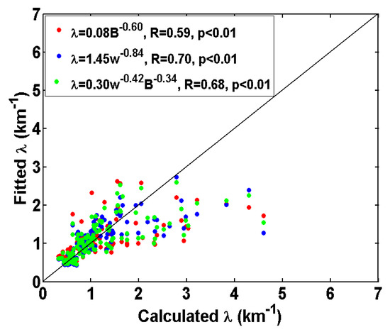
Figure 12.
Fitted entrainment rates (λ) from Equation (5) (blue points), Equation (6) (red points), and Equation (9) (green points) as a function of estimated λ. The black line denotes 1:1 isoline. The fitted function, correlation coefficient (R), and the p value of the correlation for each equation are provided, respectively, in the legend.
4. Conclusions and Discussion
This study used the mesoscale numerical model to simulate a southwest vortex precipitation process in Sichuan Basin, China, from 8 to 9 July 2010, and to calculate λ in cumulus clouds. The negative correlations between λ and dynamical factors in the cloud were used to fit λ by the power law function. The reason for the negative correlation is that, on the one hand, by reducing the temperature difference between inside and outside the cloud, entrainment decreases B, and then vertical upward motion weakens. On the other hand, the enhancement of B and upward movement means that the cloud takes less time to rise a certain distance, which reduces the chance for clouds to interact with the environment, so λ becomes smaller.
When PDF is used to fit λ, there are differences in the empirical parameters of the fitting function for different PDF ranges. When PDF is larger, the change rate of λ with dynamic parameter is larger. In addition, the slope of the log-linear fitting function decreases for developing and enhancing cumulus clouds, which is related to the strengthening of updraft motion and the decrease in λ. Because large-scale models cannot identify individual cumulus clouds with small horizontal scales, our studies average all qualified 2D clouds according to cloud top heights and then obtain the average λ, w, and B. If only one dynamic parameter is used, w is more suitable than B to be applied to fit λ. The function combing w and B was compared with two traditional schemes, and we found that λ obtained by our fitting is between the two traditional schemes proposed by Neggers et al. [19] and Gregory [20]. In addition, when the principal component regression method combines the w and B simultaneously to fit λ, the fitting effect is almost the same as that when only w is used. However, principal component regression considers the interaction between more dynamic factors and λ, so the fitting function including w and B is suitable for fitting λ in the parameterization scheme for cumulus clouds.
Our parameterization schemes are based on a case simulation, so the schemes have some inevitable limitations and uncertainties to some extent. To enhance the applicability of the parameterization schemes, more simulation cases and model settings, such as ensemble modeling by incorporating random stochastic perturbations, need to be combined to test the scheme. In addition, it is also an interesting topic to investigate the relationship between parameterization schemes and topography or environment so that the scheme can be popularized and applied to plain, marine, or other terrain conditions. Furthermore, turbulence is related to the wind field [33], so besides vertical ascending motion, turbulent motion is also closely related to entrainment [26]. The turbulent dissipation rate (ɛ) is the rate at which the turbulent kinetic energy is converted into the kinetic energy of molecular thermal motion under molecular viscosity. As we all know, B is the primary driver of w and ɛ, so a larger B usually results in a larger ɛ. On the other hand, turbulence at the cloud boundary could create a drag force to decrease w. So, ɛ should be an essential factor in λ parameterization scheme and must be tested under multiple conditions in the future.
Author Contributions
X.G. and H.L. performed the simulation; X.G., J.Z. and F.W. participated in data analysis and result discussion; X.G. and H.L. wrote the paper. All authors have read and agreed to the published version of the manuscript.
Funding
This research was funded by the Suzhou science and technology program project (SS2019033).
Institutional Review Board Statement
Not applicable.
Informed Consent Statement
Not applicable.
Data Availability Statement
Not applicable.
Conflicts of Interest
The authors declare no conflict of interest.
References
- Wang, Y.; Zhou, L.; Hamilton, K. Effect of convective entrainment/detrainment on the simulation of the tropical precipitation diurnal cycle. Mon. Weather Rev. 2007, 135, 567–585. [Google Scholar] [CrossRef]
- Lu, C.; Liu, Y.; Niu, S.; Vogelmann, A.-M. Empirical relationship between entrainment rate and microphysics in cumulus clouds. Geophys. Res. Lett. 2013, 40, 2333–2338. [Google Scholar] [CrossRef]
- Gao, S.; Lu, C.; Liu, Y.; Mei, F.; Wang, J.; Zhu, L.; Yan, S. Contrasting scale dependence of entrainment-mixing mechanisms in stratocumulus clouds. Geophys. Res. Lett. 2020, 47, e2020GL086970. [Google Scholar] [CrossRef]
- Gao, S.; Lu, C.; Liu, Y.; Yum, S.-S.; Zhu, J.; Zhu, L.; Desai, N.; Ma, Y.; Wu, S. Comprehensive quantification of height dependence of entrainment mixing between stratiform cloud top and environment. Atmos. Chem. Phys. 2021, 21, 11225–11241. [Google Scholar] [CrossRef]
- Lu, C.; Zhu, L.; Liu, Y.; Mei, F.; Fast, J.-D.; Pekour, M.-S.; Luo, S.; Xu, X.; He, X.; Li, J. Observational study of relationships between entrainment rate, homogeneity of mixing, and cloud droplet relative dispersion. Atmos. Res. 2023, 293, 15. [Google Scholar] [CrossRef]
- Luo, S.; Lu, C.; Liu, Y.; Gao, W.; Zhu, L.; Xu, X.; Li, J.; Guo, X. Consideration of initial cloud droplet size distribution shapes in quantifying different entrainment-mixing mechanisms. J. Geophys. Res. Atmos. 2021, 126, e2020JD034455. [Google Scholar] [CrossRef]
- Yao, M.-S.; Del Genio, A.-D. Effects of cumulus entrainment and multiple cloud types on a January global climate model simulation. J. Clim. 1989, 2, 850–863. [Google Scholar] [CrossRef]
- Xu, X.; Sun, C.; Lu, C.; Liu, Y.; Zhang, G.; Chen, Q. Factors affecting entrainment rate in deep convective clouds and parameterizations. J. Geophys. Res. Atmos. 2021, 126, e2021JD034881. [Google Scholar] [CrossRef]
- Xu, X.; Lu, C.; Liu, Y.; Luo, S.; Zhou, X.; Endo, S.; Zhu, L.; Wang, Y. Influences of an entrainment–mixing parameterization on numerical simulations of cumulus and stratocumulus clouds. Atmos. Chem. Phys. 2022, 22, 5459–5475. [Google Scholar] [CrossRef]
- Luo, S.; Lu, C.; Liu, Y.; Bian, J.; Gao, W.; Li, J.; Xu, X.; Gao, S.; Yang, S.; Guo, X. Parameterizations of entrainment-mixing mechanisms and their effects on cloud droplet spectral width based on numerical simulations. J. Geophys. Res. Atmos. 2020, 125, e2020JD032972. [Google Scholar] [CrossRef]
- Turner, J.-S. The motion of buoyant elements in turbulent surroundings. J. Fluid Mech. 1963, 16, 1–16. [Google Scholar] [CrossRef]
- Tiedtke, M.-A. Comprehensive Mass Flux Scheme for Cumulus Parameterization in Large-Scale Models. Mon. Weather Rev. 1989, 117, 1779–1800. [Google Scholar] [CrossRef]
- Siebesma, A.-P.; Cuijpers, J.-W.-M. Evaluation of parametric assumptions for shallow cumulus convection. J. Atmos. Sci. 1995, 52, 650–666. [Google Scholar] [CrossRef]
- Bechtold, P.; Köhler, M.; Jung, T.; Doblas-Reyes, F.; Leutbecher, M.; Rodwell, M.-J.; Vitart, F.; Balsamo, G. Advances in simulating atmospheric variability with the ECMWF model: From synoptic to decadal time-scales. Q. J. Roy. Meteor. Soc. 2008, 134, 1337–1351. [Google Scholar] [CrossRef]
- Bretherton, C.-S.; McCaa, J.-R.; Grenier, H. A new parameterization for shallow cumulus convection and its application to marine subtropical cloud-topped boundary layers. Part I: Description and 1-D results. Mon. Weather Rev. 2004, 132, 864–882. [Google Scholar] [CrossRef]
- De Rooy, W.-C.; Siebesma, A.-P. A simple parameterization for detrainment in shallow cumulus. Mon. Weather Rev. 2008, 136, 560–576. [Google Scholar] [CrossRef]
- Stirling, A.-J.; Stratto, R.-A. Entrainment processes in the diurnal cycle of deep convection over land. Q. J. Roy. Meteor. Soc. 2012, 138, 1135–1149. [Google Scholar] [CrossRef]
- Bera, S.; Prabha, T.-V. Parameterization of Entrainment Rate and Mass Flux in Continental Cumulus Clouds: Inference from Large Eddy Simulation. J. Geophys. Res. Atmos. 2019, 124, 13127–13139. [Google Scholar] [CrossRef]
- Neggers, R.-A.-J.; Siebesma, A.-P.; Jonker, H.-J.-J. A multiparcel model for shallow cumulus convection. J. Atmos. Sci. 2002, 59, 1655–1668. [Google Scholar] [CrossRef]
- Gregory, D. Estimation of entrainment rate in simple models of convective clouds. Q. J. Roy. Meteor. Soc. 2001, 127, 53–72. [Google Scholar] [CrossRef]
- Del Genio, A.-D.; Wu, J. The role of entrainment in the diurnal cycle of continental convection. J. Clim. 2010, 23, 2722–2738. [Google Scholar] [CrossRef]
- Von Salzen, K.; McFarlane, N.A. Parameterization of the bulk effects of lateral and cloud-top entrainment in transient shallow cumulus clouds. J. Atmos. Sci. 2002, 9, 405–1430. [Google Scholar] [CrossRef]
- Lin, C. Some bulk properties of cumulus ensembles simulated by a cloud-resolving model. Part II: Entrainment profiles. J. Atmos. Sci. 1999, 56, 3736–3748. [Google Scholar] [CrossRef]
- Dawe, J.-T.; Austin, P.-H. Direct entrainment and detrainment rate distributions of individual shallow cumulus clouds in an LES. Atmos. Chem. Phys. 2013, 13, 7795–7811. [Google Scholar] [CrossRef]
- Zhang, G.; Wu, X.; Zeng, X.; Mitovski, T. Estimation of convective entrainment properties from a cloud-resolving model simulation during TWP-ICE. Clim. Dyn. 2015, 47, 2177–2192. [Google Scholar] [CrossRef]
- Lu, C.; Liu, Y.; Zhang, G.; Wu, X.; Endo, S.; Cao, L.; Li, Y.; Guo, X. Improving Parameterization of Entrainment Rate for Shallow Convection with Aircraft Measurements and Large-Eddy Simulation. J. Atmos. Sci. 2016, 73, 761–773. [Google Scholar] [CrossRef]
- Romps, D.-M.; Kuang, Z. Nature versus nurture in shallow convection. J. Atmos. Sci. 2010, 67, 1655–1666. [Google Scholar] [CrossRef]
- Li, Y.W.; Niu, S.J. The formation and precipitation mechanism of two ordered patterns of embedded convection in stratiform cloud. Sci. China Earth Sci. 2012, 55, 113–125. [Google Scholar] [CrossRef]
- Shahi, N.-K.; Polcher, J.; Bastin, S.; Pennel, R.; Fita, L. Assessment of the spatio-temporal variability of the added value on precipitation of convection-permitting simulation over the Iberian Peninsula using the RegIPSL regional earth system model. Clim. Dyn. 2022, 59, 471–498. [Google Scholar] [CrossRef]
- Gerber, H.-E.; Frick, G.-M.; Jensen, J.-B.; Hudson, J.-G. Entrainment, mixing, and microphysics in trade-wind cumulus. J. Meteor. Res. Jpn. 2008, 86, 87–106. [Google Scholar] [CrossRef]
- Lu, C.; Liu, Y.; Niu, S.; Vogelmann, A.-M. Observed impacts of vertical velocity on cloud microphysics and implications for aerosol indirect effects. Geophys. Res. Lett. 2012, 39, L21808. [Google Scholar] [CrossRef]
- Guo, X.; Lu, C.; Zhao, T.; Zhang, G.; Liu, Y. An observational study of entrainment rate in deep convection. Atmosphere 2015, 9, 1362–1376. [Google Scholar] [CrossRef]
- Gharaati, M.; Xiao, S.; Wei, N.J.; Martínez-Tossas, L.-A.; Dabiri, J.-O.; Yang, D. Large-eddy simulation of helical-and straight-bladed vertical-axis wind turbines in boundary layer turbulence. J. Renew. Sustain. Energy. 2022, 14, 5. [Google Scholar] [CrossRef]


Disclaimer/Publisher’s Note: The statements, opinions and data contained in all publications are solely those of the individual author(s) and contributor(s) and not of MDPI and/or the editor(s). MDPI and/or the editor(s) disclaim responsibility for any injury to people or property resulting from any ideas, methods, instructions or products referred to in the content. |
© 2023 by the authors. Licensee MDPI, Basel, Switzerland. This article is an open access article distributed under the terms and conditions of the Creative Commons Attribution (CC BY) license (https://creativecommons.org/licenses/by/4.0/).