Diurnal Evolution and Estimates of Hourly Diffuse Radiation Based on Horizontal Global Radiation, in Cerrado-Amazon Transition, Brazil

Abstract

In the Cerrado-Amazonian ecotone in the State of Mato Grosso, intensely altered by anthropic action, the knowledge and processes of energy conversion and energy balance are still incipient, making the monitoring and modeling of diffuse radiation essential for several applications. The objective of this study was to evaluate the seasonality of the diurnal evolution and estimate the hourly diffuse radiation ($H_d^h)$ and incident radiation in the horizontal plane between June 2011 and October 2016. The instantaneous measurements (5 min) of diffuse radiation underwent geometric, astronomical, and anisotropic corrections, with subsequent hourly integrations. The seasonality of diffuse radiation and its radiometric fractions was evaluated. The estimates were made considering total and seasonal data groupings (water stations in the region) and in different cloudiness classes (atmospheric transmissivity index—$K_T^h$). The diurnal behavior of diffuse radiation ($H_d^h$) was similar to that of global radiation and at the top of the atmosphere, with maximum values at solar noon. The correlations between $K_d^h$ and $K_T^h$ showed third-order polynomial behavior, with maximum observed values of $K_d^h$ ranging from 0.8 to 0.9, for $K_T^h$ less than 0.2. Estimation equations based on radiometric fractions underestimated the values of diffuse radiation, with a better performance presented by models adjusted in annual data groupings. Among the parameterized models for estimating diffuse radiation obtained in the literature, those calibrated regionally in this study, together with those developed for tropical regions, presented better statistical performances.

1. Introduction

Brazil is in full technological development in the areas of renewable energy (photothermal and photovoltaic conversion, biomass and biodiesel), agriculture (increased efficiency based on the physical and physiological properties of crops and animals), and civil construction (construction materials, micrometeorological aspects), among others. This Brazilian scenario reflects what happens worldwide, with continuous increases in energy supply and demand, especially from renewable sources, due to limited fossil fuel resources and the problems associated with greenhouse gases [1]. In this context, solar energy plays an important role in the global and national sustainable infrastructure [2], being considered a clean energy source that does not use fuels with fossil origins [3].

The need to supply energy on an ever-increasing scale, and at the same time economically and sustainably, together with the profile of the high national agrosilvopastoral potential, make up a growing demand for the knowledge of seasonal variations in solar radiation levels, considering the spectral and atmospheric attenuation components in the Brazilian territory. The temporal variation of the amount of solar radiation incident at any location on the Earth’s surface depends on astronomical, geographic, and atmospheric factors. The main variations in the seasonal levels of each component of solar radiation originate from the interaction with the atmosphere since some atmospheric constituents are relatively constant in concentration (permanent gases), and others are highly variable in time and space (such as CO₂, methane, aerosols, and water vapor). This variability allows the current composition and concentration of gases in the atmosphere to depend on the geographic position, altitude, and time of year, influencing solar radiation’s absorption, reflection, and transmission. In turn, among the local characteristics, variations in altitude, inclination (declivity), orientation (azimuth), and shading can affect the energy levels available on the surface, mainly with changes in the geometry of incidence of direct solar fluxes [4,5].

The solar radiation that reaches the earth’s surface, called global radiation, can be divided into two components, direct and diffuse, which are transmitted directly through the atmosphere (without attenuation) and result from the scattering action in the atmosphere, respectively [6,7]. Measurements of global radiation fluxes are normally obtained in the horizontal plane and are available in instantaneous, hourly, daily, monthly, and annual partitions.

Diffusion is a fundamental physics process associated with electromagnetic waves and their interaction with matter, in which particles in the path of an electromagnetic wave radiate their energy in all directions, occurring for all wavelengths within the electromagnetic spectrum. The size of the particles interferes directly in the dispersion process, given by the proportion between the circumference of the particle and the incident wavelength (λ), that is, x = 2πa/λ (where ‘a’ is the radius of the particle); in this case, if x < 1 (when the particle diameter is less than 10% of the size of the incident wavelength), the dispersion is called selective or isotropic (Rayleigh scattering). For particles whose sizes are similar to or larger than the wavelength, i.e., x ≥ 1, the diffusion is known as non-selective or anisotropic (Mie scattering) [4,5].

In Brazil, the knowledge of diffuse radiation levels is restricted to locations close to research institutions and universities since the country does not have a solarimetric monitoring network. Recently, the main Brazilian studies focused specifically on the characterization and estimation of diffuse radiation were developed in the Southeast regions [8,9,10,11,12,13,14,15], Northeast [16,17,18], and South [19,20,21]. Through a partnership between the Federal University of Mato Grosso and the Laboratory of Solar Radiometry of the Faculty of Agricultural Sciences of UNESP, between 2011 and 2016, global and diffuse radiation monitoring was carried out at the Federal University of Mato Grosso, University Campus of Sinop, standing out as the only site with these observations in the northern region of Mato Grosso [22,23]. This article presents the quantification of energy levels of diffuse radiation in this locality, in hourly temporal partitions, and in different seasonal periods, in addition to contributing to the understanding of the behavior of local atmospheric phenomena, serves as an environmental indicator since it reflects the air load of aerosols in suspension because of anthropic activities such as forest fires.

In several parts of the world, as well as in Brazil, the global radiation is measured in horizontal planes in many locations, however, the beam and diffuse radiation data can be obtained in restricted periods and are very scarce. The diffuse solar radiation levels generally follow the seasonal radiation behavior at the top of the atmosphere and vary throughout the year according to local atmospheric conditions (precipitation, cloudiness, aerosols, among other factors) [24]. The greatest difficulties in obtaining diffuse radiation are linked to the variation in cloudiness, for conditions ranging from clear to cloudy skies; under clear sky conditions they can be calculated theoretically using various climatic and geographic (local) parameters. However, there is not good method for computing the diffuse radiation under a cloudy sky. Regarding this topic, many researchers have recently carried out several studies with empirical formulas based on different parameters for different regions of the world [3,25,26,27], new estimation methodologies such as machine learning models and hybrids models [28,29,30,31,32], and remote sensing applications [33,34].

This work aimed to analyze the seasonality and propose statistical models for estimating the hourly diffuse radiation incident on the horizontal in the Cerrado-Amazon transition, Mato Grosso state, Brazil. For this purpose, the annual and seasonal diurnal evolution of global and diffuse radiation and their radiometric fractions were characterized; in addition, statistical models for estimating hourly diffuse radiation were calibrated based on the atmospheric transmissivity coefficient, and comparisons were made with parameterized models that allow the estimation of hourly diffuse radiation.

2. Materials and Methods

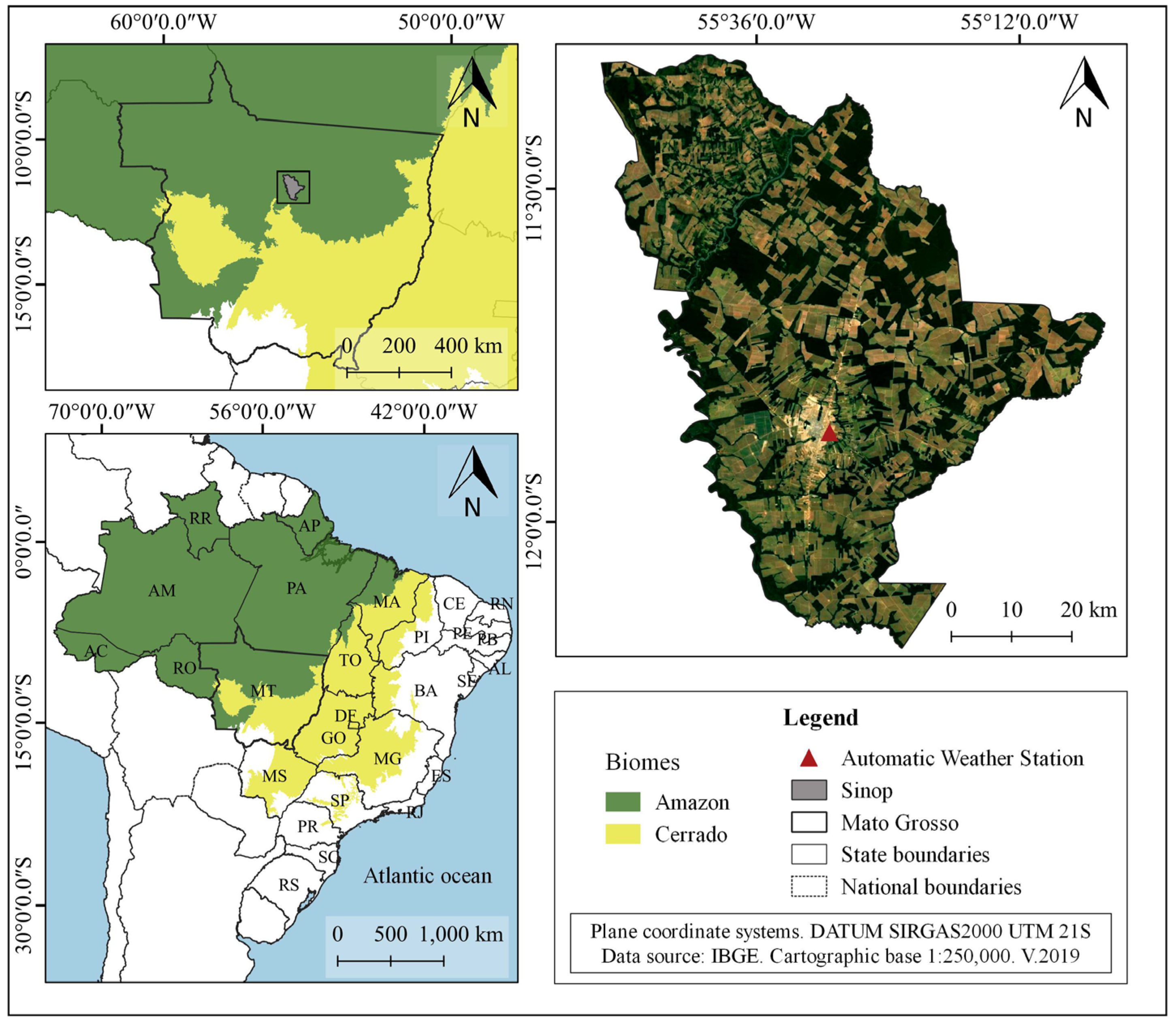
2.1. Characterization of the Study Region

Global and diffuse radiation data, as well as other meteorological variables used in this study, were obtained from an Automatic Meteorological Station (AMS) in Sinop, Mato Grosso, located at latitude 11.864° S and longitude 55.485° W (altitude 371 m) (Figure 1). The evaluated database provides measures between June 2011 and October 2016, which, despite being short and not updated, is representative of the atmospheric behavior of the region, as it is a 5-year time series.

The municipality of Sinop is located in the Mid-North Region of the State of Mato Grosso, spanning 3942.23 km² with approximately 130,000 inhabitants. With large population growth in the last seven years (around 20%), the use and occupation of the soil has been intensely altered, with the conversion of vegetated areas into urban and agricultural areas and an increase in the demand for energy and other natural resources [35].

According to the Köppen climate classification, the climate of the region is hot and humid Aw tropical, characterized by the presence of two well-defined seasons: rainy (October to April) and dry (May to September) [36]. Average monthly temperatures range between 22.9 and 25.8 °C, with an annual average of 24.7 °C, and annual precipitation totals are around 2000 mm. There is a high similarity between the average monthly seasonality of meteorological variables recorded during the study period (06/2011 to 10/2016) by AMS UFMT Sinop and the climatological norm of the region (Figure 2). For the representation of the norms, a historical series of the Gleba Celeste station was used, which, despite being located in a neighboring municipality (Vera-MT), distant around 80 km, presents the oldest data set in the region (1972 to 2010).

For the observational characterization of the seasonality of global and diffuse radiation, it was decided to group the months according to the rainfall regime of the region, avoiding the seasonal evaluation by the seasons. This type of seasonal analysis is favorable in regions with frequent atmospheric changes resulting from rainfall patterns, as recommended by [37] for the analysis of solar radiation estimates in the Amazon. Souza et al. [36] emphasized that the State of Mato Grosso is representative of great environmental complexity, conditioned, among other factors, to water availability. By observing the behavior of rainfall (Figure 2), the following groupings were adopted: (i): rainy season (December to February); (ii) dry season (June to August); (iii) rainy/dry transition (March to May); (iv) dry/rainy transition (September to October).

2.2. Instrumentation and Data Analysis

Instantaneous global and diffuse radiation data (5-min values) were monitored by Kipp and Zonen CM3 pyranometers positioned at a height of 1.0 m on a metallic platform (Figure 3). The sensors had a response sensitivity of ±10–35 μV/Wm², a response time of 18 s, a temperature response of ±1.0% for the range from −40 to 80 °C, and deviations for the cosine effect of ±2% (0 < z < 80°). Data were recorded by a CR1000 datalogger (Campbell Scientific, Logan, UT, USA), operating at 1 Hz of frequency. For the measurement of diffuse radiation, the pyranometer was positioned under the MEO shading ring [38], constantly remaining below the shadow projected by the ring. In contrast, for global radiation the measurement, the sensor remained in full sun. The shading ring used was 0.1 m wide and 0.4 m in radius.

In addition to the pyranometers and MEO shading ring, the following sensors were used: psychrometer with thermometric shelter Vaisala CS 215 installed at 2 m height, Vaisala TE 525 rain gauge at 1.5 m height, heliograph at 1.5 m height, for the monitoring meteorological elements of air temperature and air relative humidity, rainfall, and insolation, respectively.

The solar radiation data were submitted for analysis to observe inconsistencies generated by the collection and storage system. By integrating instantaneous partitions, global ($H_G^h$) and diffuse ($H_d^h$) hourly irradiation were obtained. The hourly extraterrestrial radiation ($H_0^h$) was obtained according to Iqbal [4]. After the hourly integrations, the $H_d^h$ data were submitted to geometric and astronomical corrections proposed by Dal Pai [39] and Oliveira et al. [40] by applying the isotropic/geometric correction factor—FC (Equations (1) and (2)). For the location, FC ranges from 0.99 to 1.00. Anisotropic correction factors proposed by Dal Pai et al. [12,41] are dependent on atmospheric transmissivity ($H_T^h$), following the sky cover classification described by Escobedo et al. [42] (

Table 1. Anisotropic correction factors for diffuse radiation by the MEO shading ring method.

${\mathit{K}}_{\mathit{T}}^{\mathit{h}}$ Range	Sky Cover	Correction Factor
0 ≤ $K_T^h$< 0.35	Cloudy	0.975
0.35 ≤ $K_T^h$ < 0.55	Partially cloudy	1.034
0.55 ≤ $K_T^h$ < 0.65	Partially clear	1.083
$K_T^h$ ≥ 0.65	Clear	1.108

Source: Dal Pai et al. [12].

).

$$FC=\frac{1}{1-Fp}$$

(1)

$$Fp=\left(\frac{2b}{\pi R}\right).cos\left(\delta \right).{\left[\frac{cos\left(\phi +\delta \right)}{cos\left(\phi \right)}\right]}^2.{\int }_0^{w_S}cos\left(\theta z\right)d\omega$$

(2)

where: Fp represents the portion of diffuse radiation intercepted by the shading ring; b—ring width (0.1 m); R—ring radius (0.4 m); δ—solar declination; w—hour angle; ϴ_Z—zenith angle.

Next, the hourly database was filtered, considering the criteria described by Escobedo et al. [42], where: (i) $H_G^h$/$H_0^h$< 0.82 and (ii) $H_d^h$/$H_G^h$< 1.0. After processing the data (n = 23,704 h of observation of solar radiation), a sample “n” of 22,506 h was obtained, that is, there was a loss of approximately 5% of the data.

2.3. Radiometric Fractions of Diffuse Radiation

The hourly atmospheric transmissivity coefficients ($K_T^h$) and the radiometric fractions $K_d^h$ and $K_d^{h\prime }$were obtained (Equations (3), (4), and (5), respectively).

$$K_T^h=\frac{H_G^h}{H_0^h}$$

(3)

$$K_d^h=\frac{H_d^h}{H_G^h}$$

(4)

$$K_d^{h\prime }=\frac{H_d^h}{H_0^h}$$

(5)

Subsequently, statistical equations were generated for the correlations between the hourly global radiation diffuse fraction ($H_G^h$) and the atmospheric transmissivity coefficient ($K_T^h$) for the annual and seasonal data groupings (four hydrological seasons). In this case, the data series was divided into two parts (in a 2:1 ratio) for calibration/generation and statistical performance analysis of the estimates (validation). In this case, an organization was adopted so that the months were contemplated proportionally in the two databases, resulting in 42 and 23 months for generation and validation, respectively, uniformly distributed over the years.

The correlations between $K_d^h$ and $K_T^h$allowed adjustments of third-order polynomials, as recommended by Abreu et al. [43]. Polynomial regression equations were also generated for the $K_T^h$ intervals 0 ≤ $K_T^h$< 0.55 (which includes cloudy and partially cloudy sky coverage) and $K_T^h$ ≥ 0.55 (partly open and open sky) to improve the performance of the estimates. The $K_d^h$ × $K_T^h$correlations were generated in total (annual) and seasonal grouping of data.

2.4. Estimates of Diffuse Radiation by Parameterized Models

The correlations proposed in this study were compared with 17 parameterized models for estimating hourly diffuse radiation based on the $K_d^h$ × $K_T^h$ correlation available in the literature for the most different regions of the globe (

Table 2. Description of hourly diffuse radiation estimation models used in this study.

Equation Number	Authors (Reference)	Local	${\mathit{K}}_{\mathit{T}}^{\mathit{h}}$ Range	Equations/Values
1	Boland et al. [45]	Geelong, Australia (−38.09°; 144.34°)	0 ≤ $K_T^h$ ≤ 1	$K_d^h=1/[1+exp(7.997\left(K_T^h-0.586\right)]$
2	Boland; Ridley [46]	Adelaide (−34.92°; 138.59°) and Geelong (−38.09°; 144.34°)—Australia	0 ≤ $K_T^h$ ≤ 1	$K_d^h=1/[1+\mathit{exp}\left(-5+8.60K_T^h\right)]$
3	Boland; Ridley [46] adjusted	Rio de Janeiro, Brazil (−22.86°; −43.23°)	0 ≤ $K_T^h$ ≤ 1	$K_d^h=1/[1+\mathit{exp}\left(-4.90+8.78K_T^h\right)]$
4	Erbs et al. [47]	EUA (31.08° to 42.42°; −71.48° to −121.70°)	$K_T^h$ ≤ 0.22	$K_d^h=1-0.09K_T^h$
5			0.22 < $K_T^h$ ≤ 0.8	$K_d^h=0.9511-0.1604K_T^h\pm {4.388K_T^h}^2-16.638K_T^h³+12.336K_T^{h4}$
6			$K_T^h$ > 0.8	$K_d^h=0.165$
7	Furlan et al. [8]	São Paulo, Brazil (−23.56°; −46.73°)	$K_T^h$ < 0.228	$K_d^h=0.961$
8			$K_T^h$ ≥ 0.228	$K_d^h=1.337-1.65K_T^h$
9	Jacovides et al. [48]	Athalassa, Cyprus (34.61° to 35.61°; 32° to 34.5°)	$K_T^h$ ≤ 0.1	$K_d^h=0.987$
10			0.1< $K_T^h$ ≤ 0.8	$K_d^h=0.94+0.937K_T^h-{5.01K_T^h}^2+3.32K_T^h³$
11			$K_T^h$ > 0.8	$K_d^h=0.165$
12	Lam; Li [49]	Hong Kong, China (22.3°; 114.3°)	$K_T^h$ < 0.15	$K_d^h=0.977$
13			0.15 ≤ $K_T^h$ ≤ 0.7	$K_d^h=1.237-1.361K_T^h$
14			$K_T^h$ > 0.7	$K_d^h=0.273$
15	Maduekwe; Chendo [50]	Lagos, Nigeria (6.46°; 3.40°)	0 ≤ $K_T^h$ ≤ 0.3	$K_d^h=1.021-0.151K_T^h$
16			0.3 < $K_T^h$ < 0.8	$K_d^h=1.385-1.396K_T^h$
17			$K_T^h$ ≥ 0.8	$K_d^h=0.295$
18	Maduekwe; Garba [51]	Zaria, Nigeria (11.10°; 7.68°)	$K_T^h$ ≤ 0.18	$K_d^h=1.009-0.273K_T^h$
19			0.18 < $K_T^h$ < 0.68	$K_d^h=1.077-1.136K_T^h$
20			$K_T^h$ ≥ 0.68	$K_d^h=0.292$
21		Lagos, Nigeria (6.58°; 3.33°)	$K_T^h$ ≤ 0.20	$K_d^h=1.002-0.028K_T^h$
22			0.20 < $K_T^h$ < 0.78	$K_d^h=1.336-1.369K_T^h$
23			$K_T^h$ ≥ 0.78	$K_d^h=0.314$
24	Marques Filho et al. [13]	Rio de Janeiro, Brazil (−22.86°; −43.23°)	0 ≤ $K_T^h$ ≤ 1	$K_d^h=0.13+0.86\frac{1}{1+exp(-6.29+12.26K_T^h)}$
25	Oliveira et al. [52]	São Paulo, Brazil (−23.56°; −46.73°)	$K_T^h$ ≤ 0.17	$K_d^h=1$
26			0.17< $K_T^h$ ≤ 0.75	$K_d^h=0.97+0.8K_T^h-3{K_T^h}^2-3.1{K_T^h}^3+5.2{K_T^h}^4$
27			$K_T^h$ > 0.75	$K_d^h=0.17$
28	Orgill; Hollands [53]	Toronto, Canada (43.65°; −79.38°)	$K_T^h$ < 0.35	$K_d^h=1-0.249K_T^h$
29			0.35 ≤ $K_T^h$ ≤ 0.75	$K_d^h=1.577-1.84K_T^h$
30			$K_T^h$ > 0.75	$K_d^h=0.177$
31	Reindl et al. [54]	EUA (42.7°; −73.8 and 28.4°; −80.6°) Europa (51.9° to 59.5°; 10° to 12.6°)	$K_T^h$ < 0.3	$K_d^h=1.02-0.248K_T^h$
32			0.3 ≤ $K_T^h$ ≤ 0.78	$K_d^h=1.45-1.67K_T^h$
33			$K_T^h$ > 0.78	$K_d^h=0.147$
34	Soares et al. [55]	São Paulo, Brazil (−23.56°; −46.73°)	$K_T^h$ ≤ 0.17	$K_d^h=1$
35			0.17< $K_T^h$ ≤ 0.75	$K_d^h=0.9+1.1K_T^h-4.5{K_T^h}^2+0.01{K_T^h}^3+3.14{{K_T^h}^4}^{}$
36			$K_T^h$ > 0.75	$K_d^h=0.17$
37	Spencer [44]	Melbourne, Australia (−37.82°; 144.97°)	$K_T^h$< 0.35	$K_d^h=0.85$
38			0.35 ≤ $K_T^h$ ≤ 0.75	$K_d^h=1.352-1.668K_T^h$
39			$K_T^h$ > 0.75	$K_d^h=0.10$
40	Spencer [44], adjusted	Sinop, Brazil (−11.86°; −55.48°)	$K_T^h$ < 0.35	$K_d^h=0.68$
41			0.35 ≤ $K_T^h$ ≤ 0.75	$K_d^h=1.08-1.35K_T^h$
42			$K_T^h$ > 0.75	$K_d^h=0.07$

). Some of the models are partitioned, with estimation equations for different $K_T^h$ intervals, totaling 42 equations. The table presents the location for which the equations were developed, and the corresponding $K_T^h$ intervals. Spencer’s [44] equations were adjusted for local latitude.

2.5. Statistical Performance Evaluations of Estimation Models

In evaluating the performance of the estimation equations and models, the statistical indicators MBE (Mean Bias Error), RMSE (Root Mean Square Error), and Willmott’s “d” and the coefficient of determination (R²) (Equations (6)–(9), respectively), were indicated by Abreu et al. [43] as the most used.

$$MBE=\frac{\sum _{i=1}^{n}Pi-Oi}{n}$$

(6)

$$RMSE={\left[\frac{\sum _{i=1}^n{\left(P_i-O_i\right)}^2}{n}\right]}^{0.5}$$

(7)

$$d=1-\frac{\sum _{i=1}^n{\left(P_i-O_i\right)}^2}{\sum _{i=1}^n{\left(\left|{P\prime }_i-\overline{O}\right|+\left|{O\prime }_i-\overline{O}\right|\right)}^2}$$

(8)

$$R^2=\frac{{SQ}_{Reg}}{{SQ}_{TOTAL}}$$

(9)

where: Pi—estimated values; Oi—measured values; N—number of observations; |P′i|—absolute value of the difference Pi—$\overline{O}$; |O′i|—absolute value of the difference Oi—$\overline{O}$; SQ—sum of squares (obtained from simple linear regression ANOVA).

In evaluating the performance of the estimation equations and models, the statistical indicators MBE (Mean Bias Error), RMSE (Root Mean Square Error), and Willmott’s “d” and the coefficient of determination (R²) (Equations (6) to (9)) were indicated by Abreu et al. [43] as the most used.

The MBE and RMSE values represent, respectively, the mean deviation and the actual value of the error produced by the model. Negative MBE values indicate underestimations of the tested model, and vice versa. The smaller the absolute value of MBE, the better the performance of the tested model. The same applies to the RMSE. The concordance index “d” reflects the precision of the estimated values of the observed ones. It takes values between 0 to 1, and the closer to 1, the more perfect the agreement. The determination coefficient measures how well the model describes the observed data—the higher the value, the more adequate the proposed model is [56,57,58].

3. Results

3.1. Radiations and Fractions Radiometrics

Figure 4 presents the annual diurnal evolution of $H_0^h$, $H_G^h$, and $H_d^h$ and their respective standard deviations. It is observed that the behavior of global and diffuse radiation is the same as that of incident radiation at the top of the atmosphere, with maximum values at solar noon and minimum values at sunrise and sunset. Mean $H_0^h$, $H_G^h$, and $H_d^h$ values at 12 h are 4.57 ± 0.03, 2.25 ± 0.12, and 0.53 ± 0.21 MJ m⁻² h⁻¹, respectively. In the hours of rising and setting sun, the average values observed for $H_0^h$are 0.35 ± 0.07 and 0.41 ± 0.06 MJ m⁻² h⁻¹, and for $H_G^h$ they are 0.04 ± 0.03 and 0.08 ± 0.02 MJ m⁻² h⁻¹; being the global radiation incident at these times practically composed only by the diffuse portion ($H_d^h$ = 0.03 ± 0.04 and 0.06 ± 0.00 at 6 a.m. and 6 p.m., respectively).

The photoperiod during the dry and wet/dry transition seasons is shorter due to zenith variations. The seasonal average values of $H_G^h$ and $H_d^h$ follow the same behavior as $H_0^h$, with maximums for radiation at the top of the atmosphere during the rainy season (December/January/February) and minimums in the dry season (June/July/August), both at 12 h (means of $H_0^h$: 4.98 ± 0.01 and 4.07 ± 0.00 MJ m⁻² h⁻¹, respectively).

For global radiation, the maximum mean values were observed at solar noon in the dry season 2.47 ± 0.13 MJ m⁻² h⁻¹. A similar behavior is observed by Marques Filho et al. [13] in a study conducted in the city of Rio de Janeiro-RJ (−22.86°; −43.23°), justified by the fact that the reduction in precipitation in the dry period is related to the decrease in cloud cover, which raises the levels of $H_G^h$.

Due to the high cloudiness during the rainy season, the lowest averages of $H_G^h$ and the highest averages of $H_d^h$ (at solar noon) were also observed in this period, 2.02 ± 0.15 and 0.66 ± 0.17 MJ m⁻² h⁻¹, respectively. The minimum averages of $H_d^h$ at solar noon occur in the dry period 0.35 ± 0.04 MJ m⁻² h⁻¹. The lowest standard deviation values for global and diffuse radiation are observed during the dry season due to the greater stability of atmospheric conditions (

Table 3. Diurnal evolution of diffuse radiation ($H_d^h$) in different seasonal periods, in the region of Sinop, MT, between 2011–2016.

Solar Time (Hour)	Rainy		Rainy/Dry		Dry		Dry/Rainy
	Average	SD	Average	SD	Average	SD	Average	SD
5	-	-	-	-	-	-	-	-
6	0.0208	0.00	-	-	-	-	0.0353	0.01
7	0.1705	0.04	0.1152	0.02	0.0919	0.02	0.1973	0.04
8	0.3910	0.09	0.3490	0.05	0.2334	0.13	0.3847	0.06
9	0.5209	0.11	0.4680	0.16	0.2706	0.08	0.4762	0.09
10	0.5993	0.16	0.5370	0.22	0.2706	0.03	0.5210	0.11
11	0.6377	0.19	0.6022	0.23	0.3199	0.04	0.5520	0.14
12	0.6634	0.17	0.6262	0.20	0.3527	0.04	0.5661	0.15
13	0.6351	0.13	0.6207	0.19	0.3860	0.05	0.5614	0.16
14	0.5733	0.06	0.5573	0.14	0.3665	0.04	0.5333	0.12
15	0.5243	0.07	0.4929	0.14	0.3140	0.02	0.4956	0.10
16	0.4406	0.06	0.3925	0.12	0.2486	0.02	0.3937	0.06
17	0.2846	0.05	0.2430	0.09	0.2017	0.06	0.2352	0.04
18	0.1067	0.02	-	-	-	-	0.0516	0.02
19	-	-	-	-	-	-	-	-

Abbreviation: SD = standard deviation.

).

Figure 5 shows the annual diurnal evolution of the radiometric fractions $K_T^h$, $K_d^h$, and $K_d^h\prime$ during the four hydrological seasons. The maximum value of atmospheric transmissivity of global radiation occurs at solar noon, with incident radiation levels on the Earth’s surface corresponding to approximately 50% of $H_0^h$. The minima were observed at sunrise for a better analysis of atmospheric transmissivity throughout the year.

$K_d^h$ has the opposite behavior to $K_T^h$, with higher values at the beginning and end of the day. At these times, global radiation is predominantly composed of diffuse radiation, corresponding to about 70% of energy levels (67.66% and 75.22%, respectively). The hourly average values of $K_d^h$range from 0.15 to 0.78, with a higher hourly average in the rainy season (0.53 ± 0.13) due to the higher concentration of water vapor in the atmosphere. The lower values of standard deviations for $K_d^h$in the dry season are justified by the greater stability in atmospheric conditions.

The atmospheric transmissivity coefficient $K_T^h$ranges from 0.07 to 0.64, with a higher average value in the dry season (0.53 ± 0.14) due to low cloud cover, which allows for greater passage of direct radiation. The lowest mean value, consequently, is observed in the rainy season, 0.33 ± 0.11, while in the transition seasons $K_T^h$ranges from 0.36 to 0.42.

Through the analysis of the average values of $K_T^h$, and according to the sky cover classification established by Escobedo et al. [42], it can be stated that the behavior of the sky in Sinop, in the dry season, varies from cloudy to partially cloudy at the beginning of the day, and during the hours it is partially open. In the rainy season, the sky remains cloudy or partially cloudy throughout the day.

In all hydrological stations, the sky is cloudy in the early morning, with a reduction in the atmospheric transmissivity coefficient at the end of the day, except in the dry season, when $K_T^h$ values remain high. Marques Filho et al. [13] stated that the high values of $K_T^h$ at the end of the day are due to surface reflections due to the low values of the solar elevation angle at this time of year.

Table 4. Hourly mean values of radiation (MJ m⁻² h⁻¹) and radiometric fractions (dimensionless) at solar noon and at different hydrological stations, in Sinop, MT, Brazil, between 2011 and 2016.

Radiation	Rainy	Rany/Dry	Dry	Dry/Rainy
$H_0^h$	4.98 ± 0.01	4.48 ± 0.01	4.07 ± 0.00	4.86 ± 0.02
$H_G^h$	2.02 ± 0.15	2.10 ± 0.08	2.47 ± 0.13	2.29 ± 0.13
$H_d^h$	0.66 ± 0.17	0.63 ± 0.20	0.35 ± 0.04	0.57 ± 0.15
Radiometric Fraction	Rainy	Rany/Dry	Dry	Dry/Rainy
$K_T^h$	0.41 ± 0.03	0.47 ± 0.02	0.61 ± 0.03	0.47 ± 0.03
$K_d^h$	0.39 ± 0.09	0.34 ± 0.12	0.16 ± 0.02	0.28 ± 0.08
$K_d^h\prime$	0.13 ± 0.03	0.14 ± 0.04	0.09 ± 0.01	0.12 ± 0.03

describes the hourly average values of the components and fractions of solar radiation at 12 noon in the different hydrological stations.

Zamadei et al. [59] observed the diurnal evolution of $K_T^h$ in the municipality of Juína-MT, 360 km from Sinop, MT, between 10/2007 and 01/2013, and found that the highest values of $K_T^h$ occurred when the Sun had an angle of elevation greater than 45° in relation to the surface, being higher in winter (dry period). As observed in this study, the greatest deviations occurred in the afternoon, indicating an increase in the water vapor content in the atmosphere due to the evapotranspiration process that occurred in the region throughout the day. According to these authors, the highest frequencies of clear skies occurred in the months of May, June, and July (dry period), while in the period from November to March there was a cloudy sky condition (rainy period), behavior similar to that observed for Sinop, MT.

In

Table 5. Frequencies of sky conditions (hourly basis) according to the classification by Escobedo et al. [42] in Sinop, MT, Brazil, between 2011 and 2016.

Hydrological Period	I	II	III	IV
	(Cloudy)	(Partially Cloudy)	(Partially Clear)	(Clear)
Rainy	54.90	31.21	9.54	4.35
Rainy/Dry	42.56	31.60	19.63	6.21
Dry	22.53	22.97	31.22	23.28
Dry/Rainy	42.45	39.47	14.92	3.16

it is possible to observe the behavior of the sky throughout the year through the frequency of $K_T^h$ within each hydrological station. In the dry season, the condition of partially open sky prevails (31.22%), while in the rest of the year, there is a greater frequency of times with cloudy sky conditions (above 42%).

3.2. Estimates Based on the Atmospheric Transmissivity Coefficient

The $K_d^h$ × $K_T^h$ correlations are displayed in Figure 6. As observed and described in the literature, with the increase in the clarity index ($K_T^h$), the diffuse fraction tends to decrease, since there is a decrease in the isotropic effects [60]. Figure 6 shows the behavior of the correlation in the different hydro stations. It is observed that in the dry season the point cloud is more concentrated for $K_T^h$ values greater than 0.4; in this season, sky conditions II, III, and IV predominate (

Table 6. Third-degree polynomial regression coefficients and coefficients of determination (R²), in different data groups, for estimates of $K_d^h$ based on $K_T^h$.

${\mathit{K}}_{\mathit{T}}^{\mathit{h}}$ Interval	Period	Equation	R2
0 ≤ $K_T^h$ ≤ 0.82	Annual	$K_d^h=0.84197+0.1208K_T^h-4.9681{K_T^h}^2+4.84107K_T^h³$	0.8001
	Dry	$K_d^h=0.8401-0.5850K_T^h-3.0117{K_T^h}^2+3.4476K_T^h³$	0.7927
	Dry/Rainy	$K_d^h=0.8434+0.0107K_T^h-4.7464{K_T^h}^2+4.8705K_T^h³$	0.7790
	Rainy	$K_d^h=0.8567+0.4388K_T^h-6.2389{K_T^h}^2+6.1148K_T^h³$	0.7926
	Rainy/Dry	$K_d^h=0.8209+0.4635K_T^h-5.7058{K_T^h}^2+5.3027K_T^h³$	0.7737
0 ≤ $K_T^h$ < 0.55	Annual	$K_d^h=0.8249+0.5270K_T^h-6.8417{K_T^h}^2+7.0930K_T^h³$	0.7191
	Dry	$K_d^h=0.8332-0.3581K_T^h-4.2099{K_T^h}^2+5.0256K_T^h³$	0.7097
	Dry/Rainy	$K_d^h=0.8325+0.2254K_T^h-5.6085{K_T^h}^2+5.7841K_T^h³$	0.7338
	Rainy	$K_d^h=0.8333+0.9628K_T^h-8.6778{K_T^h}^2+9.1119K_T^h³$	0.7436
	Rainy/Dry	$K_d^h=0.8041+0.8778K_T^h-7.5616{K_T^h}^2+7.4359K_T^h³$	0.6989
$K_T^h$ ≥ 0.55	Annual	$K_d^h=1.7946-4.9779K_T^h+4.0593{K_T^h}^2-0.4304K_T^h³$	0.4536
	Dry	$K_d^h=1.0306-1.3726K_T^h-1.9669{K_T^h}^2+3.0059K_T^h³$	0.4302
	Dry/Rainy	$K_d^h=8.8134-39.8605K_T^h+61.3930{K_T^h}^2-31.453K_T^h³$	0.2495
	Rainy	$K_d^h=3.1103-13.0974K_T^h+19.7241{K_T^h}^2-9.9342K_T^h³$	0.0817
	Rainy/Dry	$K_d^h=2.4911-9.7927K_T^h+14.2012{K_T^h}^2-7.0667K_T^h³$	0.3154

). In the rainy season and rainy/dry transition there is greater data dispersion, indicating that for the same value of $K_T^h$ there is great variability in the values of the diffuse fraction. Borges et al. [37] observed a similar behavior in a study carried out in the State of Rondônia (−10.75°; −62.35°), attributing this fact to the greater atmospheric variations (cloudiness) that occur during the seasons.

The lowest values of the diffuse fraction when $K_T^h$ tends to 0 can be attributed to the lower horizontal brightness in this region when compared to places at high altitudes and with rugged relief. According to Perez and Seals [61], the horizon zone is infinitesimally thin at 0° elevation.

The equations generated for the entire $K_T^h$ interval (0 to 0.82) performed better than the sectioned ones, with R² above 0.77. In this same interval, the dry and rainy seasons presented better adjustments, which indicates that the atmospheric conditions in the transition periods are more unstable, making estimates difficult. This instability can be explained by the high load of aerosols from biomass burning, an anthropic activity with greater incidence in the months of April and September, corresponding to the periods in question.

The values of the statistical indicators MBE, RMSE and Willmott’s d for the estimation equations generated can be observed in

Table 7. Statistical performance indicators of the hourly diffuse solar radiation estimation equations, generated through the $K_d^h$ × $K_T^h$ correlation in different data groups in Sinop, MT, Brazil.

		Seasonal			Annual
${\mathit{K}}_{\mathit{T}}^{\mathit{h}}$ Interval	Period	MBE	RMSE	d	MBE	RMSE	d
		(kJ m−2 h−1)	(kJ m−2 h−1)		(kJ m−2 h−1)	(kJ m−2 h−1)
0 ≤ KT ≤ 0.82	Dry	−1.3193	128.8759	0.8146	34.8982	135.2091	0.8262
	Dry/Rainy	−8.4224	155.0778	0.8813	−20.0378	158.9490	0.8727
	Rainy	43.3050	190.1991	0.8441	9.0484	183.1416	0.8418
	Rainy/Dry	−12.2662	179.9711	0.8700	−38.2923	184.0373	0.8566
	Annual				−2.7689	164.4550	0.8620
0 ≤ KT < 0.55	Dry	−9.5501	112.7701	0.8995	21.3870	113.5406	0.9116
	Dry/Rainy	−7.7196	152.1405	0.8965	−6.0579	152.7036	0.8959
	Rainy	53.6976	189.7712	0.8534	30.0348	179.8730	0.8592
	Rainy/Dry	−19.0742	173.9316	0.8957	−38.8433	178.2260	0.8850
	Annual				0.0482	160.7589	0.8918
KT ≥ 0.55	Dry	5.7624	141.0145	0.5982	50.6720	152.9184	0.6318
	Dry/Rainy	1.7279	165.3808	0.5798	−71.2616	177.6153	0.5382
	Rainy	−34.0317	155.1230	0.7406	−112.2100	186.3051	0.6665
	Rainy/Dry	14.6280	206.3153	0.5297	−35.6082	203.5052	0.5082
	Annual				−8.0671	171.5742	0.6583

Abbreviations: MBE = mean bias error; RMSE = root mean square error; d = Willmott index of agreement.

. The seasonal equations, in the intervals of 0.0 ≤ $K_T^h$ ≤ 0.82 and 0.0 ≤ $K_T^h$ < 0.55, tended to underestimate the diffuse radiation values during the year. A similar behavior was observed by Borges et al. [37] and Oliveira et al. [52] in the correlations established in their studies. In the range of $K_T^h$ ≥ 0.55, there was an inversion of this behavior, with a tendency to overestimate.

Regarding the annual equations, when applied to water stations, there was also a tendency to underestimate the values of $H_d^h$, especially for $K_T^h$ ≥ 0.55. The RMSE values ranged from 112.8 to 206.3 kJ m⁻² h⁻¹, with higher scattering rates observed in the rainy season due to the high variation in atmospheric conditions.

The seasonal equations showed better statistical performances when compared to the annual ones in the same periods, except for the rainy season in the intervals 0.0 ≤ $K_T^h$ ≤ 0.82 and 0.0 ≤ $K_T^h$ < 0.55, in which the annual equation developed for each partition showed better statistical indicators than the equation for each specific period.

Regarding the annual equations applied to the entire data set, there is a tendency for underestimations in the intervals 0.0 ≤ $K_T^h$ ≤ 0.82 and $K_T^h$ ≥ 0.55, and overestimations of the values when 0.0 ≤ $K_T^h$ < 0.55. Scattering over all $K_T^h$ intervals is about 160 kJ m⁻² h⁻¹, and the fit index values are best for intervals 0.0 ≤ $K_T^h$ ≤ 0.82 and 0.0 ≤ $K_T^h$ < 0.55.

3.3. Estimates by Parameterized Models

Table 8. Statistical performance indicators of parameterized and calibrated equations in estimating hourly diffuse radiation, in Sinop, MT, Brazil, between 2011 and 2016.

Equation Number	Authors (Reference)	R²	MBE (kJ m−2 h−1)	RMSE (kJ m−2 h−1)	d	Pv1	Pv2	Pv3	Pv4	Pv5
1	Boland et al. [45]	0.66	411.04	542.52	0.5761	5	40
2	Boland; Ridley [46]	0.65	405.76	537.79	0.5804	4	38
3	Boland; Ridley [46] adjusted	0.67	355.46	479.92	0.6195	3	34
4	Erbs et al. [47]	0.13	49.66	92.55	0.9524		13	3
5		0.52	502.64	599.13	0.4815		41		8
6		-	−22.50	74.53	0.9351		6			1
7	Furlan et al. [8]	-	47.80	92.46	0.9545		11
8		0.55	323.65	414.50	0.5959		31		3
9	Jacovides et al. [48]	-	11.09	19.37	0.9874		1
10		0.68	371.30	470.10	0.5814		35		4
11		-	−22.50	74.53	0.9351		7			1
12	Lam; Li [49]	-	21.22	38.22	0.9813		2
13		0.66	388.16	478.45	0.5571		39		6
14		-	235.05	300.58	0.6069		28			10
15	Maduekwe; Chendo [50]	0.27	107.56	193.01	0.8892		22	5
16		0.43	673.86	752.01	0.3855		45		10
17		-	−16.69	53.78	0.7335		10			3
18	Maduekwe; Garba [51]	0.08	30.53	55.73	0.9735		3	1
19		0.62	334.18	426.01	0.5814		33		4
20		-	296.55	357.16	0.8663		26			8
21		0.10	42.49	78.22	0.9592		8	2
22		0.60	552.21	644.74	0.4500		43		9
23		-	148.53	201.72	0.9432		20			6
24	Marques Filho et al. [13]	0.66	323.39	444.28	0.6473	2	30
25	Oliveira et al. [52]	-	30.63	54.32	0.9724		4
26		0.63	378.78	465.83	0.5704		37		5
27		-	−25.74	110.94	0.9012		15			5
28	Orgill; Hollands [53]	0.37	141.32	258.74	0.8397		25	6		2
29		0.37	602.34	675.65	0.4151		44		10
30		-	−14.90	109.15	0.9075		9
31	Reindl et al. [54]	0.27	99.99	181.92	0.8980		21	4
32		0.44	525.15	602.22	0.4572		42		9
33		-	−73.05	118.859	0.9255		18			4
34	Soares et al. [55]	-	30.63	54.323	0.9724		5
35		0.63	329.15	416.25	0.6053		32		2
36		-	−25.74	110.94	0.9012		16			4
37	Spencer [44]	-	103.37	218.12	0.8707		23
38		0.38	357.84	441.05	0.5447		36		7
39		-	−134.08	185.07	0.6875		24			7
40	Spencer [44] adjusted	-	29.64	143.53	0.9255		17
41		0.38	181.71	285.48	0.6659		27		3
42		-	−180.52	231.66	0.5804		29			9
43	Generated model 1 *	0.79	6.32	157.93	0.8707	1	14
44	Generated model 2 *	0.70	6.52	151.16	0.9040		12		1
45	Generated model 3 *	0.05	7.51	171.60	0.6351		19			5

Abbreviations: R² = correlation coefficient; MBE = mean bias error; RMSE = root mean square error; d = Willmott index of agreement; Pv = position values; * indicate models calibrated for the location.

presents the statistical performance indicators of the 42 evaluated equations (17 models) and the three equations generated in this study (annual grouping in Table 7). In order to assess the performance of the tested estimation models, the method of position values (Pv) of the statistical indicators was used, in which weights from 1 to “n” are assigned to each statistical indicator in each model, with “n” corresponding to the number of evaluated equations. In the end, the best model (equation) is the one considered with the lowest accumulated Pv value, obtained by summing the Pv of each equation in each indicative statistic [62]. The models (equations) were classified by the accumulated value of accumulated Pv considering five groups: (1) Pv1—models with total data grouping ($K_T^h$ < 0.82); (2) Pv2—all 42 equations; (3) Pv3—models developed for cloudy sky conditions ($K_T^h$ < 0.35); (4) Pv4—intermediate sky conditions (0.35 < $K_T^h$ < 0.65); (5) Pv5—clear sky conditions ($K_T^h$ > 0.65).

The coefficients of determination (R²) obtained between values measured and estimated by the parameterized equations showed maximum values around 0.70 (some equations did not show significant correlations). Furthermore, these equations generated MBE values ranging from −180.52 to 673.86 kJ m⁻² h⁻¹ and scattering (RMSE) ranging from 19.37 to 752.01 kJ m⁻² h⁻¹, respectively. The three locally calibrated equations (equations 43 to 45) showed the lowest overestimates of hourly diffuse radiation, regardless of atmospheric transmissivity.

For the analysis of models that present sectioned regression equations for different intervals of the atmospheric transmissivity coefficient, those that determine fixed values for $K_d^h$ were disregarded. Subsequently, the statistical performance was analyzed regarding the estimate of diffuse radiation ($H_d^h$).

For cloudy sky conditions, six equations were analyzed (4, 15, 18, 21, 28, and 31), and the two models generated by Maduekwe and Garba [51] showed the best statistical performances (Table 8—Pv3 group). These equations, despite having low determination coefficients (0.08 and 0.10), were significant at 5% probability, and when compared with measured values they showed good results for the agreement index “d” (0.9735 and 0.9592) and low scattering indexes (55.73 and 78.22 kJ m⁻² h⁻¹, respectively). Oliveira et al. [63] stated that the coefficient of determination should not be used individually in the analysis of statistical performance, but can help in decision making when comparing different regression models.

For intermediate sky cover conditions (partly cloudy and partly open) fourteen equations were evaluated, and the best estimates were obtained with the equations generated in this study (Table 8—group Pv4). The models by Furlan et al. [8], Spencer [44] and Soares et al. [55], when adjusted, overestimated the diffuse radiation and presented greater scattering when compared with the results generated by equation 44. As for the open sky conditions (Table—Pv5 group), thirteen models of prediction of diffuse radiation determine fixed values for $K_d^h$, with the exception of the one generated in this study. Most of these equations tend to underestimate the diffuse fraction, except for equations 14, 20, 23, and 45. For this $K_T^h$ range (above 0.7), the models developed by Erbs et al. [47] and Jacovides et al. [48] presented better performances when compared to the others (Pv.5).

Of the ten models that showed the best performance for estimating the diffuse fraction in the different $K_T^h$ ranges, eight were developed or adjusted for tropical regions (latitudes between 6.58° and −23.56°). Of these, there were five for Brazil, which confirms the influence of this climatic factor on the diffuse radiation incident on the Earth’s surface.

4. Discussion

When comparing the annual averages of $H_d^h$ in the morning and afternoon periods, a higher value was observed during the afternoon (0.27 ± 0.21 and 0.33 ± 0.21 MJ m⁻² h⁻¹) for the morning and afternoon periods, respectively. Soil heating, and consequently evapotranspiration, are highest in the afternoon, which causes greater attenuation of solar radiation due to the high concentration of water vapor present in the atmosphere.

Diffuse radiation behaves similarly to global radiation in hydrological stations, with the exception of the dry season, in which case there is no symmetry between the morning and afternoon periods (Table 3). This behavior may be due to multireflection processes associated with the elevation of the zenith angle, especially in the first hours of sun exposure, with a reduction in the dispersion of suspended particles in the atmosphere.

The increase in the variability of the diffuse fraction of global radiation can also be attributed to a phenomenon called “cloud gap effect” [64,65,66]. According to the authors, at a given solar elevation angle, a decrease in the atmospheric transmissivity coefficient generally indicates an increase in cloud thickness. However, there is an exception when clouds are not continuously distributed across the sky. Ground surfaces illuminated by the Sun, located at the end of paths of solar beams passing through gaps formed between clouds, may receive greater irradiance than under a clear sky, due to the scattering and reflection of the radiation beam from the side of adjacent clouds. This effect can increase the irradiation incident on the ground by up to 20%. In short, you can increase the $K_T^h$ without indicating that the sky is open.

If we compare the amplitude of the $K_d^h$ × $K_T^h$ curve generated in this study (Figure 6) with that of other regions available in the literature, it is possible to notice that the highest number of points for $K_T^h$ < 0.20 is concentrated between 0.80–0.90 $K_d^h$, while in other works this value is usually above 0.90. Some authors generate sectioned regression equations, partitioning this $K_T^h$ interval with fixed values for $K_d^h$ [48,49], including in Brazil [8,52,55].

It should be noted that smaller time slices respond more sensitively and quickly to atmospheric changes, generating greater variability and detailing of the punctual distribution of solar radiation, which makes estimation difficult. These effects are minimized when values are integrated into daily and monthly partitions [39,60].

Among the five models (equations 1, 2, 3, 24, and 43) that consider the entire $K_T^h$ interval, the best estimates were obtained by the locally calibrated equation (generated in this study). In this case, the equation proposed by Marques Filho et al. [13] presented the second best accumulated Pv, however, this model was calibrated for the city of Rio de Janeiro (RJ, Brazil), which has atmospheric characteristics distinct from the Cerrado-Amazon transition region, and, therefore, presented overestimates of radiation time difference of up to 323.39 kJ m⁻² h⁻¹. It is interesting to mention that these same authors also evaluated some models evaluated in the present study [40,46,47,48] to estimate the local diffuse radiation. However, better statistical performances were observed when using the locally developed correlation model.

Singh [67] compared the efficiency of diffuse radiation estimation models considering the entire range of the atmospheric transmissivity coefficient and intervals of cloudiness classes, and concluded that, in general, the models present similar statistical performances for regions with well-defined water seasonality (rainy and dry seasons). These observations by Sing [67] corroborate those found in the present study, through the analysis of the statistical performance of the 45 equations (group Pv2), since the five aforementioned (which consider the entire $K_T^h$ value) were classified as 14th, 30th, 34th, 38th, and 40th, respectively. In this case, the equations that estimate $K_d^h$ in intermediate sky cover performed better than the others of the same model.

The diffuse radiation database obtained in the region of Sinop, MT (Brazil), can be considered short (5 years), however, it allows applications directed mainly towards the calibration of models of estimates of diffuse radiation. The studies focused on the analysis of seasonality and estimates on daily integration have already been presented by Zamadei et al. [22,23]. The network of stations of the National Institute of Meteorology (INMET) routinely monitors hourly global horizontal radiation, and, with good estimates of diffuse radiation, it is possible, by difference, to obtain information on direct radiation in horizontal planes.

The modeling of estimation equations with the insertion of a larger number of meteorological variables is recommended for future works to verify the performance in relation to the models generated in this study, and to verify the evaluation of those existing in the literature. The correlation between the diffuse fraction and the insolation ratio can also be worked on in order to propose models with an easily obtainable variable.

The models proposed in this study can contribute to the development of solar energy utilization in places where diffuse radiation measurements are not available. Thus, in today’s conditions where global warming is a threat and greenhouse gas emissions are causing warming, the use of clean energy sources such as solar energy can reduce numerous environmental, social, and economic impacts. This study can contribute to providing necessary data on cleaner and more ecologically correct production technologies. More studies can be performed on models based on satellite data for the estimation of diffuse radiation in different climatic regions where the diffuse solar component does not exist.

It should also be noted that there is an urgent need to implement a network of solarimetric stations in the Cerrado and Amazon regions, considered important Brazilian biomes. There are no scientific reports of any radiometry monitoring in the aforementioned regions. This type of monitoring is essential to guide environmental and engineering studies in the most varied areas of knowledge. These stations must, above all, routinely monitor at intervals of 5 or 10 min, in horizontal planes, the spectral components of solar radiation (ultraviolet, visible, and infrared) and diffuse, direct radiation, and reflected radiation.

5. Conclusions

The hourly diffuse radiation in the region of Sinop, MT, presents similar behavior to the incident radiation at the top of the atmosphere and globally, with maximum values at the lowest zenith angles. Seasonality indicates higher hourly diffuse radiation levels $K_d^h$ in the rainy season in the region.

The radiometric fractions also show characteristic behavior during the different water seasons. The highest values of the atmospheric transmissivity coefficient $K_T^h$ were observed in the dry season due to low cloud cover.

The $K_d^h$ × $K_T^h$ correlation established showed a peculiar behavior, with the amplitude of the curve characteristic of regions located at low latitudes (closer to the Equator). As in other studies, when $K_T^h$ tends to 0.0, $K_d^h$ tends to 1.0; however, for $K_T^h$ values lower than 0.20, the maximum observed $K_d^h$ values ranged from 0.80 to 0.90.

Polynomial equations were generated to estimate the diffuse radiation considering three intervals of $K_T^h$, and these equations presented better statistical performances when compared with parameterized equations from the literature.

Among the 17 models (42 equations) for estimating the parameterized diffuse radiation evaluated, it is recommended to use the polynomials developed in this study or the one elaborated by Marques Filho et al. [13] for estimates of the $K_d^h$ fraction, in the range of 0.0 ≤ $K_T^h$ ≤ 1.0, for regions climatically similar to the Cerrado-Amazon transition of Mato Grosso.

References

1. Ebrahimi, A.; Ghorbani, B.; Ziabasharhagh, M. Exergy and economic analyses of an innovative integrated system for cogeneration of treated biogas and liquid carbon dioxide using absorption–compression refrigeration system and ORC/Kalina power cycles through geothermal energy. Process Saf. Environ. Prot. 2022, 158, 257–281. [Google Scholar] [CrossRef]
2. Xiao, T.; Liu, C.; Wang, X.; Wang, S.; Xu, X.; Li, Q.; Li, X. Life cycle assessment of the solar thermal power plant integrated with air-cooled supercritical CO2 Brayton cycle. Renew. Energy 2022, 182, 119–133. [Google Scholar] [CrossRef]
3. Bakirci, K. Evaluation of models for prediction of diffuse solar radiation and comparison with satellite values. J. Clean. Prod. 2022, 374, 133892. [Google Scholar] [CrossRef]
4. Iqbal, M. An Introduction to Solar Radiation; Academic Press: Toronto, ON, Canada, 1983; 390p. [Google Scholar]
5. Liou, K.N. An Introduction to Atmospheric Radiation, 2nd ed.; Academic Press: San Diego, CA, USA, 2002; 583p. [Google Scholar]
6. Varejão Silva, M.A. Meteorology and Climatology; Digital Version: Recife, Brazil, 2006; 463p. [Google Scholar]
7. Khatib, T.; Mohamed, A.; Sopian, K. A review of solar energy modeling techniques. Renew. Sustain. Energy Rev. 2012, 16, 2864–2869. [Google Scholar] [CrossRef]
8. Furlan, C.; Oliveira, A.P.; Soares, J.; Codato, G.; Escobedo, J.F. The role of clouds in improving the regression model for hourly values of diffuse solar radiation. Appl. Energy 2012, 92, 240–254. [Google Scholar] [CrossRef]
9. Souza, A.P.; Escobedo, J.F. Estimates of Hourly Diffuse Radiation on Tilted Surfaces in Southeast of Brazil. Int. J. Renew. Energy Res. 2013, 3, 207–221. [Google Scholar]
10. Dal Pai, A.; Escobedo, J.F.; Dal Pai, E.; Santos, C.M. Estimation of hourly, daily and monthly mean diffuse radiation based on MEO shadowring correction. Energy Procedia 2014, 57, 1150–1159. [Google Scholar] [CrossRef] [Green Version]
11. Rossi, T.J.; Rossi, L.R.; Santos, C.M.; Silva, M.B.P.; Escobedo, J.F. Dependence of sky coverage on the global, diffuse and direct solar fractions of the infrared spectrum in Botucatu/SP/Brazil. Braz. J. Sol. Energy 2016, 7, 40–49. [Google Scholar]
12. Dal Pai, A.; Escobedo, J.F.; Dal Pai, E.; Oliveira, A.P.; Soares, J.R.; Codato, G. MEO shadowring method for measuring diffuse solar irradiance: Corrections based on sky cover. Renew. Energy 2016, 99, 754–763. [Google Scholar] [CrossRef]
13. Marques Filho, E.P.; Oliveira, A.P.; Vita, W.A.; Mesquita, F.L.L.; Codato, G.; Escobedo, J.F.; Cassol, M.; França, J.R.A. Global, diffuse and direct solar radiation at the surface in the city of Rio de Janeiro: Observational characterization and empirical modeling. Renew. Energy 2016, 91, 64–74. [Google Scholar] [CrossRef] [Green Version]
14. Basseto, E.L.; Escobedo, J.F.; Dal Pai, A. Estimation of the diffuse fraction of global irradiation with machine learning techniques. Braz. J. Sol. Energy 2018, 9, 127–136. [Google Scholar]
15. Dal Pai, A.; Dal Pai, E.; Sarnighausen, V.C.R.; Escobedo, J.F. Evaluation of anisotropic correction models for diffuse solar irradiance measured by the MEO shadow ring method. J. Renew. Sustain. Energy 2020, 12, 063701-1–063701-11. [Google Scholar] [CrossRef]
16. Pedrosa Filho, M.H.O.; Gerônimo, C.A.O. Development of models for correlation and adjustment of diffuse radiation for the rural region of Pernambuco. In Proceedings of the VII Brazilian Solar Energy Congress, Gramado, Brazil, 17–20 April 2018. [Google Scholar]
17. Salazar, G.A.; Pedrosa Filho, M.H.O. Analysis of the diffuse fraction from solar radiation values measured in Argentina and Brazil sites. In Proceedings of the Solar World Congress, Santiago, Chile, 4–7 November 2019. [Google Scholar]
18. Gomes, L.R.T.C.; Marques Filho, E.P.; Pepe, I.M.; Mascarenhas, B.S.; Oliveira, A.P.; França, J.R. Solar Radiation Components on a Horizontal Surface in a Tropical Coastal City of Salvador. Energies 2022, 15, 1058. [Google Scholar] [CrossRef]
19. Lemos, L.F.L.; Starke, A.R.; Boland, J.; Cardemil, J.M.; Machado, R.D.; Colle, S. Assessment of solar radiation components in Brazil using the BRL model. Renew. Energy 2017, 108, 569–580. [Google Scholar] [CrossRef]
20. Crotti, P.; Rampinelli, G.A. Estimation of the direct and diffuse solar components in horizontal surface for Araranguá/SC from meteorological networks. In Proceedings of the VII Brazilian Solar Energy Congress (CBENS), Gramado, Brazil, 17–20 April 2018. [Google Scholar]
21. Souza, M.B.; Tonolo, É.A.; Yang, R.L.; Tiepolo, G.M.; Urbanetz Junior, J. Determination of Diffused Irradiation from Horizontal Global Irradiation—Study for the City of Curitiba. Braz. Arch. Biol. Technol. 2019, 62, e19190014. [Google Scholar] [CrossRef]
22. Zamadei, T.; Souza, A.P.; Escobedo, J.F.; Almeida, F.T. Estimation of daily diffuse radiation based on atmospheric transmissivity and insolation ratio in the Cerrado-Amazon Transition. Braz. J. Climatol. 2018, 23, 134–151. [Google Scholar]
23. Zamadei, T.; Souza, A.P.; Almeida, F.T.; Escobedo, J.F. Daily Global and diffuse radiation in the Brazilian Cerrado-Amazon transition region. Sci. Nat. 2021, 43, e37. [Google Scholar] [CrossRef]
24. Marín, M.J.; Estellés, V.; Gómez-Amo, J.L.; Utrillas, M.P. Diffuse and Direct UV Index Experimental Values. Atmosphere 2023, 14, 1221. [Google Scholar] [CrossRef]
25. Zhu, T.; Li, J.; He, L.; Wu, D.; Tong, X.; Mu, Q.; Yu, Q. The improvement and comparison of diffuse radiation models in different climatic zones of China. Atmos. Res. 2021, 254, 105505. [Google Scholar] [CrossRef]
26. Mirzabe, A.H.; Hajiahmad, A.; Keyhani, A. Assessment and categorization of empirical models for estimating monthly, daily, and hourly diffuse solar radiation: A case study of Iran. Sustain. Energy Technol. Assess. 2021, 47, 101330. [Google Scholar] [CrossRef]
27. Paulescu, E.; Paulescu, M. Minute-Scale Models for the Diffuse Fraction of Global Solar Radiation Balanced between Accuracy and Accessibility. Appl. Sci. 2023, 13, 6558. [Google Scholar] [CrossRef]
28. Guermoui, K.; Benkaciali, S.; Gairaa, K.; Bouchouicha, K.; Boulmaiz, T.; Boland, J.W. A novel ensemble learning approach for hourly global solar radiation forecasting. Neural Comput. Appl. 2022, 34, 2983–3005. [Google Scholar] [CrossRef]
29. Lu, Y.; Zhang, R.; Wang, L.; Su, X.; Zhang, M.; Li, H.; Li, S.; Zhou, J. Prediction of diffuse solar radiation by integrating radiative transfer model and machine-learning techniques. Sci. Total Environ. 2023, 859, 160269. [Google Scholar] [CrossRef] [PubMed]
30. Nwokolo, S.C.; Obiwulu, A.U.; Ogbulezie, J.C.; Amadi, S.O. Hybridization of statistical machine learning and numerical models for improving beam, diffuse and global solar radiation prediction. Clean. Eng. Technol. 2022, 9, 100529. [Google Scholar] [CrossRef]
31. Mustafa, J.; Husain, S.; Alqaed, S.; Khan, U.A.; Jamil, B. Performance of Two Variable Machine Learning Models to Forecast Monthly Mean Diffuse Solar Radiation across India under Various Climate Zones. Energies 2022, 15, 7851. [Google Scholar] [CrossRef]
32. Olchowik, W.; Gajek, J.; Michalski, A. The Use of Evolutionary Algorithms in the Modelling of Diffuse Radiation in Terms of Simulating the Energy Efficiency of Photovoltaic Systems. Energies 2023, 16, 2744. [Google Scholar] [CrossRef]
33. Bakirci, K. Prediction of diffuse radiation in solar energy applications: Turkey case study and compare with satellite data. Energy 2021, 237, 121527. [Google Scholar] [CrossRef]
34. Zhao, S.; Xiang, Y.; Wu, L.; Liu, X.; Dong, J.; Zhang, F.; Li, Z.; Cui, Y. Simulation of Diffuse Solar Radiation with Tree-Based Evolutionary Hybrid Models and Satellite Data. Remote Sens. 2023, 15, 1885. [Google Scholar] [CrossRef]
35. IBGE (Brazilian Institute of Geography and Statistics). Demographic Census. Available online: https://www.ibge.gov.br/estatisticas/sociais/populacao/22827-censo-demografico-2022.html?edicao=35938&t=resultados (accessed on 20 May 2023).
36. Souza, A.P.; Mota, L.L.; Zamadei, T.; Martim, C.C.; Almeida, F.T.; Paulino, J. Climatic classification and climatological water balance in the State of Mato Grosso. Nativa 2013, 1, 34–43. [Google Scholar] [CrossRef]
37. Borges, G.A.; Aguiar, L.J.G.; Fischer, G.R.; Aguiar, R.G.; Oliveira, E.C.; Paim, B.L. Estimation of diffuse solar radiation under all sky conditions in southwestern Amazonia. In Proceedings of the Workshop Brazilian of Micrometeorology, Santa Maria, Brazil, 8–11 November 2017. [Google Scholar]
38. Melo, J.M.D. Development of a System to Simultaneously Measure Global, Diffuse and Direct Radiation. Ph.D. Thesis, Paulista State University, Botucatu, Brazil, 1994. [Google Scholar]
39. Dal Pai, A. Anisotropy of Diffuse Solar Irradiance Measured by the Melo-Escobedo Shading Method: Anisotropic Correction Factors and Estimation Models. Ph.D. Thesis, Paulista State University, Botucatu, Brazil, 2005. [Google Scholar]
40. Oliveira, A.P.; Machado, A.J.; Escobedo, J.F. A New Shadow-Ring Device for Measuring Diffuse Solar Radiation at the Surface. J. Atmos. Ocean. Technol. 2002, 19, 698–708. [Google Scholar] [CrossRef]
41. Dal Pai, A.; Escobedo, J.F.; Correa, F.H.P. Numerical correction for the diffuse solar irradiance by the Melo-Escobedo shadowring measuring method. In Proceedings of the Ises Solar World Congress, Kassel, Germany, 28 August–2 September 2011. [Google Scholar]
42. Escobedo, J.F.; Gomes, E.N.; Oliveira, A.P.; Soares, J. Modeling hourly and daily fractions of UV, PAR and NIR to global solar radiation under various sky conditions at Botucatu, Brazil. Appl. Energy 2009, 86, 299–309. [Google Scholar] [CrossRef]
43. Abreu, E.F.M.; Canhoto, P.; Costa, M.J. Prediction of diffuse horizontal irradiance using a new climate zone model. Renew. Sustain. Energy Rev. 2019, 110, 28–42. [Google Scholar] [CrossRef] [Green Version]
44. Spencer, J.W. A comparison of methods for estimating hourly diffuse solar radiation from global solar radiation. Sol. Energy 1982, 29, 19–32. [Google Scholar] [CrossRef]
45. Boland, J.; Scott, L.; Luther, M. Modelling the diffuse fraction of global solar radiation on a horizontal surface. Environmetrics 2001, 12, 1003–1116. [Google Scholar] [CrossRef]
46. Boland, J.; Ridley, B. Models of diffuse solar fraction. In Modelling Solar Radiation at the Earth’s Surface; Badescu, V., Ed.; Springer: Berlin/Heidelberg, Germany, 2008; pp. 193–219. [Google Scholar] [CrossRef]
47. Erbs, D.G.; Klein, S.A.; Duffie, J.A. Estimation of the diffuse radiation fraction for hourly, daily and monthly-average global radiation. Sol. Energy 1982, 28, 293–302. [Google Scholar] [CrossRef]
48. Jacovides, C.P.; Tymvios, F.S.; Assimakopoulos, V.D.; Kaltsounides, N.A. Comparative study of various correlations in estimating hourly diffuse fraction of global solar radiation. Renew. Energy 2006, 31, 2492–2504. [Google Scholar] [CrossRef]
49. Lam, J.C.; Li, D.H.W. Correlation between global solar radiation and its direct and diffuse components. Build. Environ. 1996, 31, 527–535. [Google Scholar] [CrossRef]
50. Maduekwe, A.A.L.; Chendo, M.A.C. Atmospheric turbidity and the diffuse irradiance in Lagos, Nigeria. Sol. Energy 1997, 61, 241–249. [Google Scholar] [CrossRef]
51. Maduekwe, A.A.L.; Garba, B. Characteristics of the monthly average hourly diffuse irradiance at Lagos and Zaira, Nigeria. Renew. Energy 1999, 17, 213–259. [Google Scholar] [CrossRef]
52. Oliveira, A.P.; Escobedo, J.F.; Machado, A.J.; Soares, J. Correlation models of diffuse solar-radiation applied to the city of Sao Paulo, Brazil. Appl. Energy 2002, 71, 59–73. [Google Scholar] [CrossRef]
53. Orgill, J.F.; Hollands, K.G.T. Correlation equation for hourly diffuse radiation on a horizontal surface. Sol. Energy 1977, 19, 357–359. [Google Scholar] [CrossRef]
54. Reindl, D.T.; Beckman, W.A.; Duffie, J.A. Diffuse fraction correlations. Sol. Energy 1990, 45, 1–7. [Google Scholar] [CrossRef]
55. Soares, J.; Oliveira, A.P.; Boznar, M.Z.; Mlakar, P.; Escobedo, J.F.; Machado, J. Modeling hourly diffuse solar radiation in the city of São Paulo using neural network technique. Appl. Energy 2004, 79, 201–214. [Google Scholar] [CrossRef]
56. Willmott, C.J. On the validation of models. Phys. Geogr. 1981, 2, 184–194. [Google Scholar] [CrossRef]
57. Stone, R.J. Improved statistical procedure for the evaluation of solar radiation estimation models. Sol. Energy 1993, 51, 289–291. [Google Scholar] [CrossRef]
58. Schneider, A.; Hommel, G.; Blettner, M. Linear Regression Analysis. Dtsch. Ärzteblatt Int. 2010, 107, 776–782. [Google Scholar] [CrossRef]
59. Zamadei, T.; Silva, C.C.; Walther, N.V.S.; Souza, A.P. Average monthly hourly evolution of global radiation and atmospheric transmissivity coefficient for northwest Mato Grosso. In Proceedings of the Brazilian Congress of Agrometeorology, Belém, Brazil, 2–6 September 2013. [Google Scholar]
60. Souza, A.P. Hourly Diffuse Solar Radiation Incident on Inclined Surfaces: Correction Factors, Diurnal Evolution and Estimation Models. Ph.D. Thesis, Paulista State University, Botucatu, Brazil, 2012. [Google Scholar]
61. Perez, R.; Seals, R. A new simplified version of the Perez diffuse irradiance model for tilted surfaces. Sol. Energy 1987, 39, 221–231. [Google Scholar] [CrossRef] [Green Version]
62. Souza, A.P.; Silva, A.C.; Tanaka, A.A.; Uliana, E.M.; Almeida, F.T.; Klar, A.E.; Gomes, A.W.A. Global radiation by simplified models for the state of Mato Grosso, Brazil. Pesqui. Agropecu. Bras. 2017, 52, 215–227. [Google Scholar] [CrossRef] [Green Version]
63. Oliveira, E.A. Methods for Concordance Analysis: Simulation Study and Application to Evapotranspiration Data. Ph.D. Thesis, School of Agriculture “Luiz de Queiroz”, Piracicaba, Brazil, 2016. [Google Scholar]
64. Duchon, C.E.; O’malley, M.S. Estimating Cloud Type from Pyranometer Observations. J. Appl. Meteorol. 1999, 38, 132–141. [Google Scholar] [CrossRef]
65. Gu, L.; Fuentes, J.D.; Shugart, H.H.; Staebler, R.M.; Black, T.A. Responses of net ecosystem exchanges of carbon dioxide to changes in cloudiness: Results from two North American deciduous forests. J. Geophys. Res. Atmos. 1999, 104, 31421–31434. [Google Scholar]
66. Oliveira, P.H.F.; Artaxo, P.; Pires, C.; Lucca, S.; Procópio, A.; Holben, B.; Schafer, J.; Cardoso, L.F.; Wofsy, S.C.; Rocha, H.R. The effects of biomass burning aerosols and clouds on the CO2 flux in Amazonia. Tellus 2007, 59, 338–349. [Google Scholar] [CrossRef]
67. Singh, U.P. Diffuse Radiation Calculation Methods. Master’s Thesis, Arizona State University, Tempe, AZ, USA, 2016. [Google Scholar]
Figure 1. Location of the UFMT Automatic Meteorological Station, Sinop, MT.
Atmosphere 14 01289 g001
Figure 2. Monthly averages of precipitation (A), air temperature and air relative humidity (B), insolation (C), and hot spots (D) collected in the Sinop, MT region. Data source: AMS UFMT Sinop (2011–2016) and EMC Gleba Celeste (1972–2010).
Atmosphere 14 01289 g002
Figure 3. Metallic platform (A) and positioning scheme (B) of the Melo-Escobedo “MEO” shading ring installed in the Automatic Meteorological Station of UFMT, University Campus of Sinop.
Atmosphere 14 01289 g003
Figure 4. Annual and seasonal diurnal evolution (water stations in the region) of radiation at the top of the atmosphere ( H 0 h ), global ( H G h ), and diffuse ( H d h ), and respective standard deviations, between 2011–2016, in the region from Sinop, MT.
Atmosphere 14 01289 g004
Figure 5. Annual and seasonal diurnal evolution of K T h , K d h , and K d h for the Sinop, MT, Brazil, between 2011 and 2016.
Atmosphere 14 01289 g005
Figure 6. Correlations to estimates K d h based on K T h , in Sinop, Mato Grosso, Brazil, between 2011 and 2016.
Atmosphere 14 01289 g006