Abstract
The accurate prediction of PM2.5 concentration, a matter of paramount importance in environmental science and public health, has remained a substantial challenge. Conventional methodologies for predicting PM2.5 concentration often grapple with capturing complex dynamics and nonlinear relationships inherent in multi-station meteorological data. To address this issue, we have devised a novel deep learning model, named the Meteorological Sparse Autoencoding Transformer (MSAFormer). The MSAFormer leverages the strengths of the Transformer architecture, effectively incorporating a Meteorological Sparse Autoencoding module, a Meteorological Positional Embedding Module, and a PM2.5 Prediction Transformer Module. The Sparse Autoencoding Module serves to extract salient features from high-dimensional, multi-station meteorological data. Subsequently, the Positional Embedding Module applies a one-dimensional Convolutional Neural Network to flatten the sparse-encoded features, facilitating data processing in the subsequent Transformer module. Finally, the PM2.5 Prediction Transformer Module utilizes a self-attention mechanism to handle temporal dependencies in the input data, predicting future PM2.5 concentrations. Experimental results underscore that the MSAFormer model achieves a significant improvement in predicting PM2.5 concentrations in the Haidian district compared to traditional methods. This research offers a novel predictive tool for the field of environmental science and illustrates the potential of deep learning in the analysis of environmental meteorological data.
1. Introduction
The pervasiveness of air pollution in numerous global cities poses significant threats to public health and induces sustained detrimental effects on broader ecological systems [1,2,3]. Among the various pollutants, fine particulate matter (PM2.5), with a diameter less than 2.5 μm, stands out [4,5]. Its adverse effects range from respiratory to cardiovascular diseases, underscoring the importance of developing a model that can accurately predict PM2.5 concentrations, allowing for timely prevention measures and strategic responses [6,7,8,9].
Generally, PM2.5 prediction methods are categorized into two classes: those based on physical models and those driven by data [10,11,12,13].
Physical model-based prediction methods, such as the Community Multi-scale Air Quality (CMAQ) [14,15], WRF/Chem [16,17], and Nested Air Quality Prediction Modeling System (NAQPMS) models [18,19], rely on scientific theories and equations to elucidate patterns of air pollution diffusion and transformation [20]. The strength of these models lies in their accuracy, which depends on how closely they approximate actual atmospheric conditions, and their explainability, as the predictions are based on scientific principles [21,22,23]. However, these models require a vast number of input parameters, including pollutant emission data, meteorological data, and terrain data [24,25]. The process of obtaining and processing these parameters is complex, and the models demand substantial computational resources [26].
On the other hand, data-driven prediction methods have yielded significant results with advancements in big data and computational capabilities [27,28,29]. Machine learning algorithms like Support Vector Machines (SVM) [30,31], Random Forest (RF) [32,33], and AdaBoost [34] are extensively employed in predicting PM2.5 concentrations. However, these models primarily focus on utilizing historical data from air quality monitoring stations for predictions, largely ignoring the consideration of other influencing factors, particularly meteorological variables [35]. Meteorological conditions like temperature, humidity, wind speed, and direction significantly impact PM2.5 concentrations by influencing and shaping the diffusion, mixing, and deposition processes of particulates in the air [36,37,38,39].
Recent widespread application of deep learning technologies is beginning to alter this situation [40,41,42]. Researchers have started integrating meteorological variables into the deep learning models for PM2.5 prediction, but the prevalent approach still relies on manual feature design and employs relatively traditional models such as Long Short-Term Memory (LSTM) [43,44,45] and Gated Recurrent Units (GRU) [46,47]. While these models exhibit strengths in handling the time-series characteristics of meteorological data, their capacity to excavate deep and complex features in multi-source meteorological data needs further enhancement [48,49].
The current challenge lies in the requirement of extensive domain knowledge and presupposed data structures or relationships to handle high-dimensional meteorological data, posing serious challenges to the generality and adaptability of the models [50,51,52]. Indeed, the relationship between meteorological conditions and PM2.5 concentrations is highly nonlinear and subject to complex interactions among various environmental factors [53]. This relationship could change with alterations in time and location [54]. Therefore, there is an urgent need to develop a novel prediction model that is capable of automatically extracting salient features from high-dimensional meteorological data and can adapt to changing environmental conditions.
To address these challenges, we have designed a novel deep learning model named the Meteorological Sparse Autoencoding Transformer (MSAFormer), based on the Transformer architecture and sparse autoencoding technology. The Transformer architecture, initially designed for natural language processing tasks [55], is adept at handling long-term dependencies in the input data—thanks to its powerful self-attention mechanism—and has exhibited excellent performance in many other fields [56], including environmental science [57]. On the other hand, sparse autoencoding is an effective feature learning technique that can automatically extract and learn significant features from high-dimensional data [58].
Our model comprises three core modules. Firstly, the Meteorological Sparse Autoencoding module extracts critical features from high-dimensional, multi-site meteorological data, providing key information for understanding and predicting PM2.5 concentrations. Secondly, the Meteorological Position Embedding module utilizes a one-dimensional Convolutional Neural Network (CNN) to flatten these sparse encoded features for processing in the subsequent Transformer module. Lastly, the PM2.5 Prediction Transformer module leverages the self-attention mechanism to handle time dependencies in the input data for an accurate prediction of future PM2.5 concentrations. These designs confer superior performance on our model when handling multi-source, high-dimensional, and highly temporal meteorological data, offering a new and effective tool for precise PM2.5 prediction.
2. Materials
This study relies on data from two primary sources: air pollutant concentrations, with an emphasis on PM2.5, and meteorological variables. The PM2.5 concentration data, expressed in micrograms per cubic meter (μg/m3), were sourced from the Beijing Municipal Ecological Environmental Monitoring Center (BJMEMC). This data can be accessed via their official website, http://www.bjmemc.com.cn/ (accessed on 21 March 2023). Concurrently, a set of meteorological factors were gathered from nine meteorological monitoring stations, facilitated through the National Climatic Data Center (NCDC) of the United States, an institution within the National Oceanic and Atmospheric Administration (NOAA). Global meteorological data, encompassing factors such as temperature, pressure, dew point, wind direction and speed, cloud cover, and precipitation, can be retrieved from their official website, https://www.ncei.noaa.gov/ (accessed on 17 April 2023). The meteorological factors included in the study and their corresponding units are detailed in Table 1.

Table 1.
Description and units of meteorological factors.
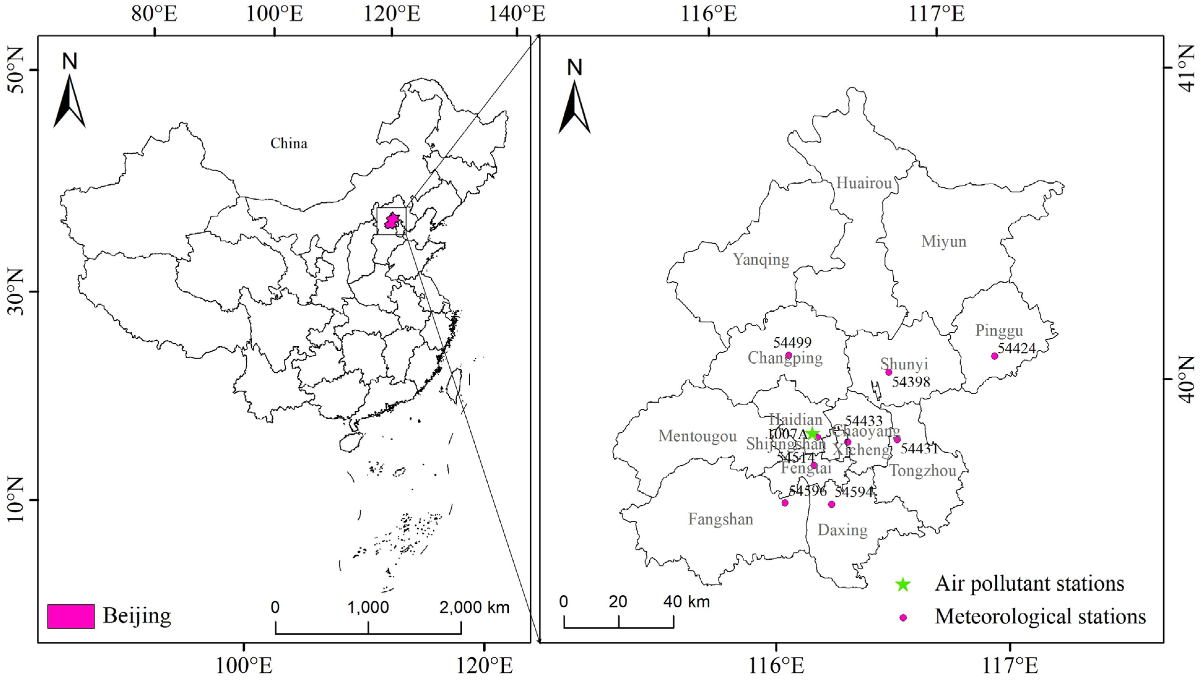
Data for the study were gathered at an hourly resolution from 1 January 2021 to 31 December 2022. The data collected from 1 January 2021 to 31 December 2021 were utilized as training data, while the data from 1 January 2022 to 31 December 2022 served as testing data. Figure 1 illustrates the geographical distribution of the meteorological and air pollutant monitoring stations from which the data was sourced.
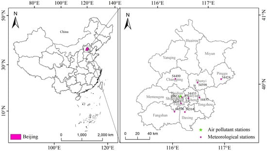
Figure 1.
Map depicting the meteorological and air pollutant monitoring stations in Beijing. The meteorological stations are represented by pink dots, while the green pentagrams denote the air pollutant monitoring stations providing the PM2.5 concentration data.
Corresponding information on these stations, such as longitude, latitude, station code, and name, is outlined in Table 2.
Table 2.
Detailed information on the meteorological and air pollutant monitoring stations used for data collection in this study.
The integration of PM2.5 concentration data from BJMEMC and meteorological data from NCDC, bolstered by comprehensive station information, provides a robust foundation for the development and validation of the MSAFormer model.
3. Methodology
3.1. Overview of the MSAFormer Model
Predicting PM2.5 concentration accurately is crucial for understanding and managing air quality in urban areas. Traditional methods, primarily based on statistical regression models, often struggle to capture complex non-linear relationships and dynamics in meteorological and pollution data. To address these challenges, we propose a novel model, MSAFormer, which combines the power of the Transformer architecture and meteorological data analysis.
MSAFormer aims to integrate meteorological and temporal information effectively to achieve an accurate prediction of PM2.5 concentration. Meteorological data, captured from various monitoring stations, provide essential contextual information related to air quality. Temporal data, reflected in the time-series data of PM2.5 concentration, reveal the dynamics of air quality over time.
To harness the rich information embedded in both meteorological and temporal data, the MSAFormer model is designed with three primary modules: the Meteorological Sparse Autoencoding module, the Meteorological Embedding module, and the Transformer Prediction module.
The Meteorological Sparse Autoencoding module is designed to encode high-dimensional meteorological data into a sparse representation. The sparsity constraint facilitates the extraction of meaningful and critical features, improving the interpretability of the model.
Next, the Meteorological Embedding module receives the sparse-encoded meteorological data, flattens them, and applies a 1D Convolutional Neural Network to encode positional information. This module transforms the encoded meteorological data into a format that is suitable for processing in the subsequent Transformer module.
Finally, the Transformer Prediction module integrates the meteorological data processed by the Meteorological Embedding module with the historical PM2.5 concentration data. The module employs the self-attention mechanism, capturing the temporal dependencies in the input data and predicting future PM2.5 concentrations.
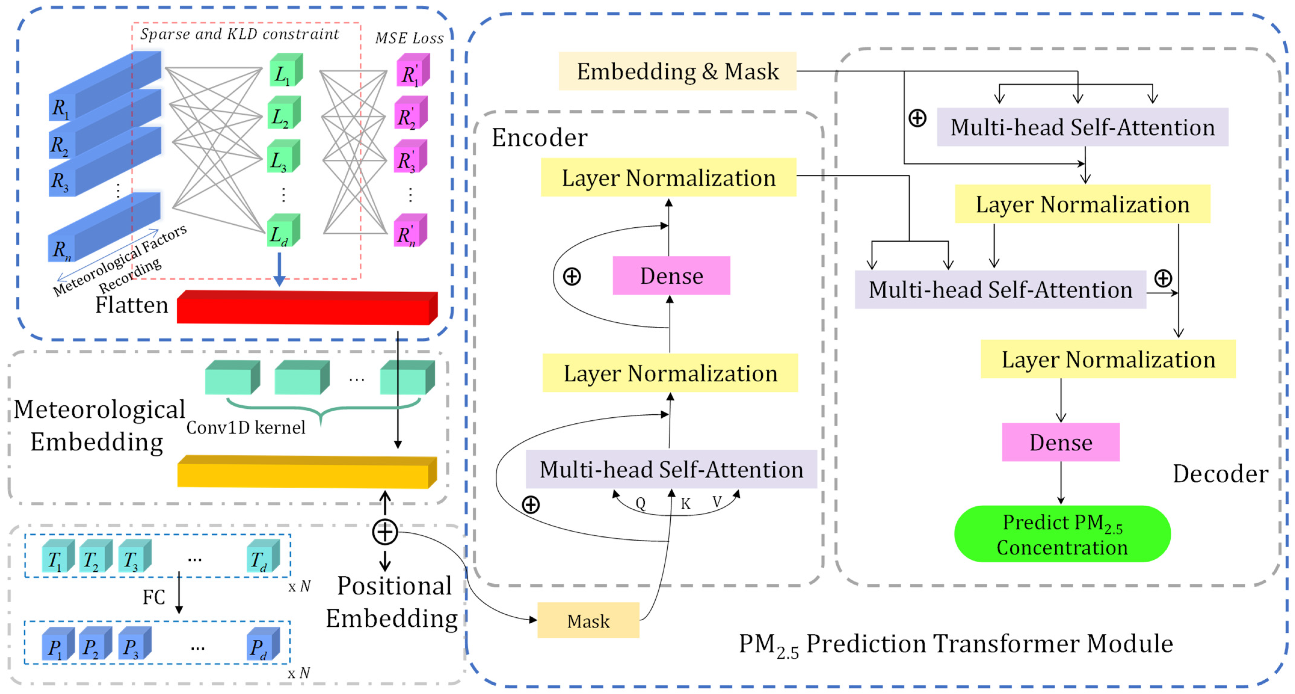
An overview of the MSAFormer model structure is provided in Figure 2, highlighting the journey of the data from the input stage, through each module, to the final prediction of PM2.5 concentration. This modular design allows for flexibility and adaptability, making the MSAFormer model a promising tool for air quality prediction tasks.
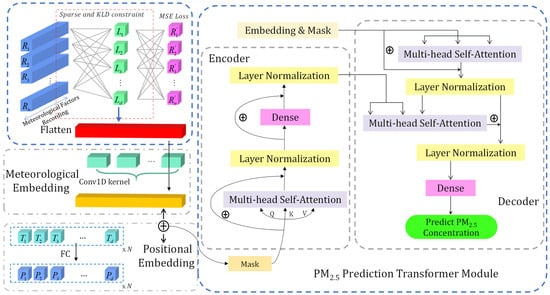
Figure 2.
Architecture of the MSAFormer model. This diagram illustrates the three key components of the MSAFormer model: the Meteorological Sparse Autoencoding module (for extracting sparse representations of meteorological data), the Meteorological Embedding module (for flattening and encoding position information via a 1D Convolutional Neural Network), and the Transformer Prediction module (for integrating meteorological and historical PM2.5 concentration data to predict future concentrations). The arrows indicate the flow of information through the model, from the input data to the final prediction of PM2.5 concentration.
3.2. Meteorological Sparse Autoencoding Module
The first module of the MSAFormer, the Meteorological Sparse Autoencoding module, deals with the processing of multivariate meteorological data. This module employs the concept of sparse autoencoding to transform the original high-dimensional meteorological data into a reduced, more manageable feature space that emphasizes critical information and suppresses noise and redundant features.
Consider the raw meteorological data collected from nine meteorological stations across Beijing. For each station, we have a time series of several meteorological features, namely temperature, pressure, dew point, wind speed, wind direction, cloud cover, and precipitation. Hence, for each station, we formulate a matrix , where is the number of meteorological features, and is the number of time steps.
A typical sparse autoencoder comprises two components: an encoder , parameterized by , and a decoder , parameterized by . The encoder aims to transform the high-dimensional input data into a lower-dimensional representation , where is the number of latent features.
The decoder, on the other hand, tries to reconstruct the original input from the encoded representation, i.e., . The goal of the training process is to minimize the reconstruction error while maintaining the sparsity of the encoded representation .
To achieve this, we employ a loss function that combines the reconstruction error, given using the Frobenius norm of the difference between the original and reconstructed matrices, and a sparsity-inducing penalty term based on the Kullback–Leibler (KL) divergence. The loss function is thus given using:
where denotes the Frobenius norm, represents the KL divergence between the empirical distribution of and the specified sparse prior distribution , and is a tunable parameter that controls the balance between the reconstruction error and the sparsity.
The Meteorological Sparse Autoencoding module plays a vital role in the MSAFormer model, as it effectively condenses high-dimensional meteorological data into a lower-dimensional, sparse, and informative representation. This representation serves as the foundation for the following modules to build upon and produce accurate PM2.5 predictions.
3.3. Meteorological Positional Embedding Module
Once the sparse-encoded representations of the meteorological data are obtained through the Meteorological Sparse Autoencoding module, we next transform these features into a form suitable for the Transformer Prediction module. The Meteorological Embedding module accomplishes this by employing a 1D Convolutional Neural Network (CNN) to capture local dependencies among the meteorological features and convert the multi-dimensional input data into a flat representation. Additionally, a fully connected layer (FC) is utilized to encode positional information into the flattened data.
Let us denote the sparse-encoded representation of the meteorological data from the previous module as , where is the dimension of the sparse-encoded representation, and is the number of time steps. The sparse-encoded data are organized into a matrix that needs to be reformatted for the time-series prediction task.
To leverage the inherent local dependencies in the multi-dimensional meteorological data, we apply a 1D convolution over the dimension of the sparse-encoded data. The 1D convolution operation uses a set of learnable filters to perform a sliding dot product over the input data. This mechanism allows the model to learn local patterns in the meteorological features.
Mathematically, the 1D convolution operation can be defined as follows. Given an input and a filter , the convolution operation outputs a new representation , where each element is computed using
After the 1D convolution operation, the flattened meteorological features are passed through a fully connected layer to encode positional information into the data. The FC layer essentially applies a linear transformation to the input data and can be represented as:
where and are the weight matrix and bias vector of the FC layer, respectively, and is the output dimension.
The output of this module, the embedded meteorological data, thus preserves critical information from the sparse-encoded representation but also incorporates local meteorological dependencies and positional information. This form of data proves to be more suitable for processing in the next Transformer Prediction module, ultimately contributing to more accurate PM2.5 predictions.
3.4. PM2.5 Prediction Transformer Module
Following the Meteorological Embedding module, the Transformer Prediction module is applied to perform PM2.5 prediction. The embedded meteorological data from the previous module, along with the historical PM2.5 data, are used as inputs for this module. The Transformer architecture is known for its ability to capture complex dependencies in sequential data and provide robust and interpretable predictions. Therefore, it is well-suited for handling our time-series prediction task.
The Transformer module contains an encoder and a decoder, both of which are composed of several identical layers. Each layer comprises two sub-layers: a multi-head self-attention mechanism and a position-wise fully connected feed-forward network. An essential feature of the Transformer is that it replaces the recurrence mechanism with the self-attention mechanism, which computes a weighted sum of all the input features rather than processing the input data step by step. This mechanism gives the model the capacity to focus more on important features and less on unimportant ones.
In the context of our model, let us denote the output from the Meteorological Embedding module as and the historical PM2.5 data as , where is the output dimension of the Meteorological Embedding module, is the dimension of the historical PM2.5 data, and is the number of time steps. The Transformer Prediction module processes these data in the following way:
- Encoder: The encoder takes the Meteorological Embedding module’s output as an input and passes it through the multi-head self-attention mechanism and the feed-forward network. The self-attention mechanism allows the model to focus on different parts of the input sequence and considers their importance for the current prediction. The feed-forward network further processes the attended features;
- Decoder: The decoder receives the encoded meteorological data and the historical PM2.5 data . Similar to the encoder, it also contains a multi-head self-attention mechanism and a feed-forward network; however, it has an additional multi-head attention mechanism that attends to the encoder’s output.
The decoder ultimately generates a sequence of predicted PM2.5 values. The Transformer Prediction module harnesses the complex temporal dependencies in both meteorological and historical PM2.5 data, contributing to the generation of accurate and robust PM2.5 predicts.
3.5. Training Strategy
The architecture and optimization parameters in the MSAFormer model play critical roles in achieving a high accuracy in PM2.5 concentration predictions. The architecture parameters are specifically configured to optimally capture the spatial and temporal dynamics within multi-station meteorological data. Table 3 presents a detailed configuration of the architecture parameters.
Table 3.
Architecture parameters for MSAFormer model.
The Sequence Window Size of 5 was chosen to balance the trade-off between capturing enough temporal dependencies and computational efficiency. For the Conv1D Kernel Size, a setting of 7 was found to be effective for learning the inherent patterns in the meteorological data. Both Conv1D Embedding Size and Position Embedding Size are set to 128, which ensures an integrated and comprehensive representation of the meteorological and spatial information. The Transformer module, with eight attention heads and four layers, can capture the complex patterns and dependencies within the data at various abstraction levels. Model optimization is carried out using an adaptive learning strategy combined with a suitable loss function. The primary optimization parameters are presented in Table 4.
Table 4.
Optimization parameters for MSAFormer model.
Adam optimizer is used for its adaptive learning rate adjustment capability, which aids efficient and robust optimization. We employ the Mean Squared Error (MSE) loss function, which is formulated as
where represents the observed PM2.5 concentration, the predicted concentration, and n the total number of samples. This loss function aligns with our goal of minimizing prediction error in PM2.5 concentration.
Furthermore, we incorporated an early stopping strategy to monitor the validation loss during training. When the validation loss stops improving after a certain number of epochs (patience), the training process is halted. This strategy helps in preventing overfitting by not allowing the model to learn the noise within the training data.
In summary, the training and optimization strategies employed in MSAFormer ensure its robustness and reliability in predicting PM2.5 concentrations using multi-station meteorological data. These strategies contribute to the model’s ability to generalize well to unseen data, making it a practical tool for air quality prediction tasks.
4. Results and Discussion
4.1. Data Preparation and Evaluation Metrics
This study assembled an extensive dataset comprising hourly observations of PM2.5 concentrations from 1 January 2021 to 31 December 2022. Initially, the PM2.5 concentration data were transformed into serialized samples using the sliding window method, with a Sequence Window Size of 5 for single-step prediction. Any serialized samples with missing PM2.5 concentrations were then carefully eliminated to ensure data integrity. Next, meticulous data cleaning procedures were implemented for the meteorological factors. The SimpleImputer class from the scikit-learn package was employed to address any missing values, replacing them with the mean, median, or most frequent value, as appropriate. After ensuring the continuity and coherence of the dataset through these cleaning processes, temporal alignment was performed to synchronize the serialized PM2.5 concentration samples with corresponding meteorological features, resulting in a set of 16,000 valid samples. These samples were then temporally divided into a training dataset (spanning the period from 1 January 2021 to 31 December 2021) and a testing dataset (from 1 January 2022 to 31 December 2022).
In the context of our study, the prediction problem is formulated as follows: Given the past 5 h of PM2.5 and meteorological factor data, the goal is to predict the PM2.5 concentration for the next hour. Mathematically, this can be defined as
where and represent the past 5 h of PM2.5 and meteorological factor data, respectively, and denotes the prediction model.
The performance of the models is evaluated using Root Mean Squared Error (RMSE), Mean Absolute Error (MAE), and the Coefficient of Determination (). These metrics are defined as
where denotes the number of samples, and represent the actual and predicted PM2.5 concentrations, respectively, and stands for the mean of the actual PM2.5 concentrations. The objective of our study is to minimize RMSE and MAE while maximizing the score.
4.2. Models Comparation and Performance Analysis
In order to establish the efficacy of the proposed MSAFormer model, it was juxtaposed against five widely recognized models: Support Vector Machine (SVM) [30], Random Forest (RF) [32], Adaptive Boosting (AdaBoost) [34], Long Short-Term Memory (LSTM) [43], and Gated Recurrent Unit (GRU) [46]. These models are detailed below:
- Support Vector Machine (SVM): This was implemented employing a radial basis function (RBF) kernel. The optimal parameters, C and gamma, were ascertained via a grid search over the parameters of ‘C’: [0.1, 1, 10, 100, 1000] and ‘gamma’: [1, 0.1, 0.01, 0.001, 0.0001];
- Random Forest (RF): the RF model was constructed with a forest of 100 trees, with ‘max_features’ set to ‘sqrt’, a choice guided by the nature of regression tasks;
- Adaptive Boosting (AdaBoost): AdaBoost was set up with 50 weak learners, with a learning rate of 1, ensuring an efficient trade-off between bias and variance;
- Long Short-Term Memory (LSTM): the LSTM, a popular variant of recurrent neural networks, was structured with 50 units, and the activation function was set as ‘tanh’;
- Gated Recurrent Unit (GRU): GRU, a modern variant of recurrent neural networks, shared the same structure as LSTM, with 50 units and a ‘tanh’ activation function.
The temporal dynamics and predictive performance of the six models were compared using three evaluation methods: time-series visualization, accuracy metrics, and error histogram analysis.
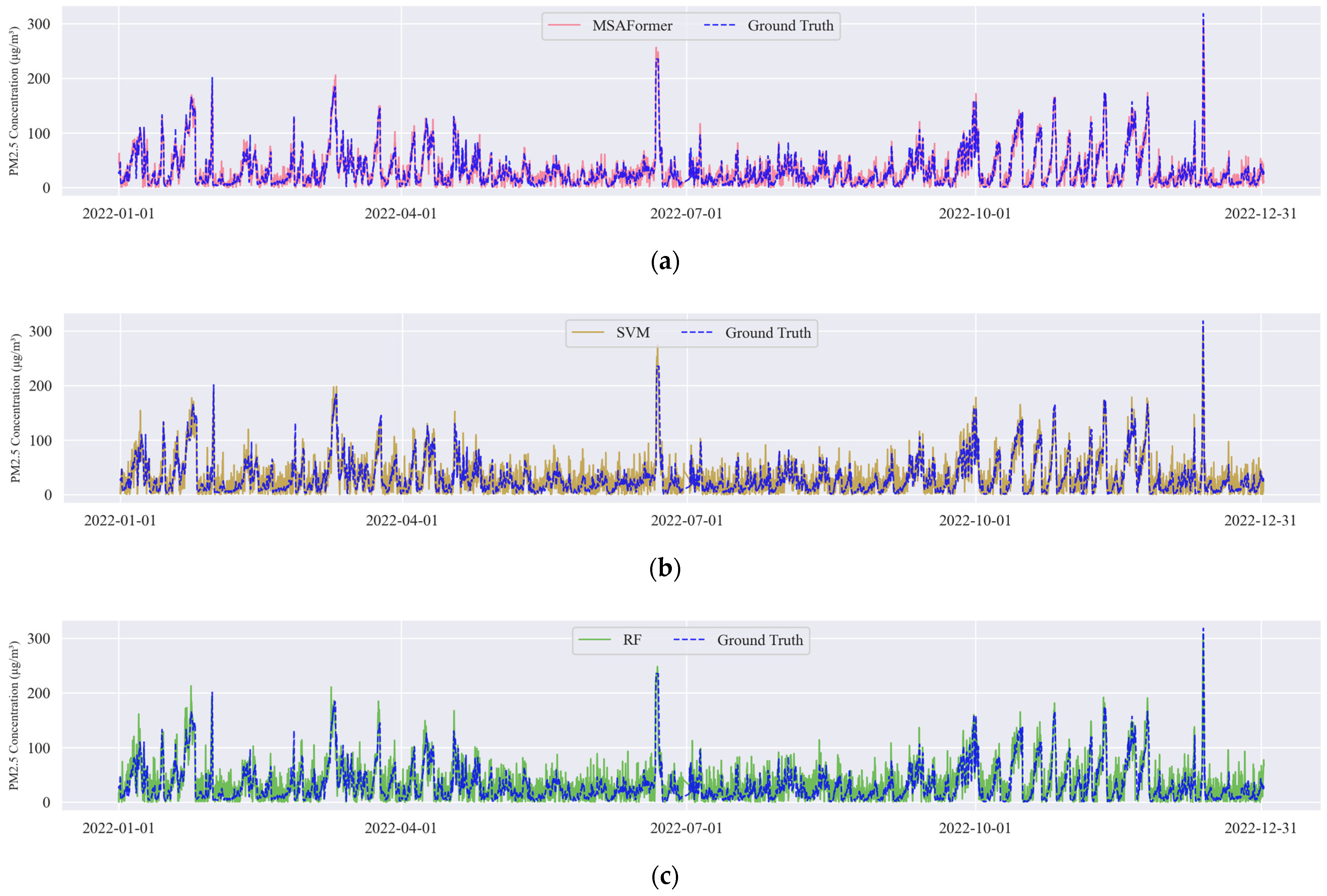
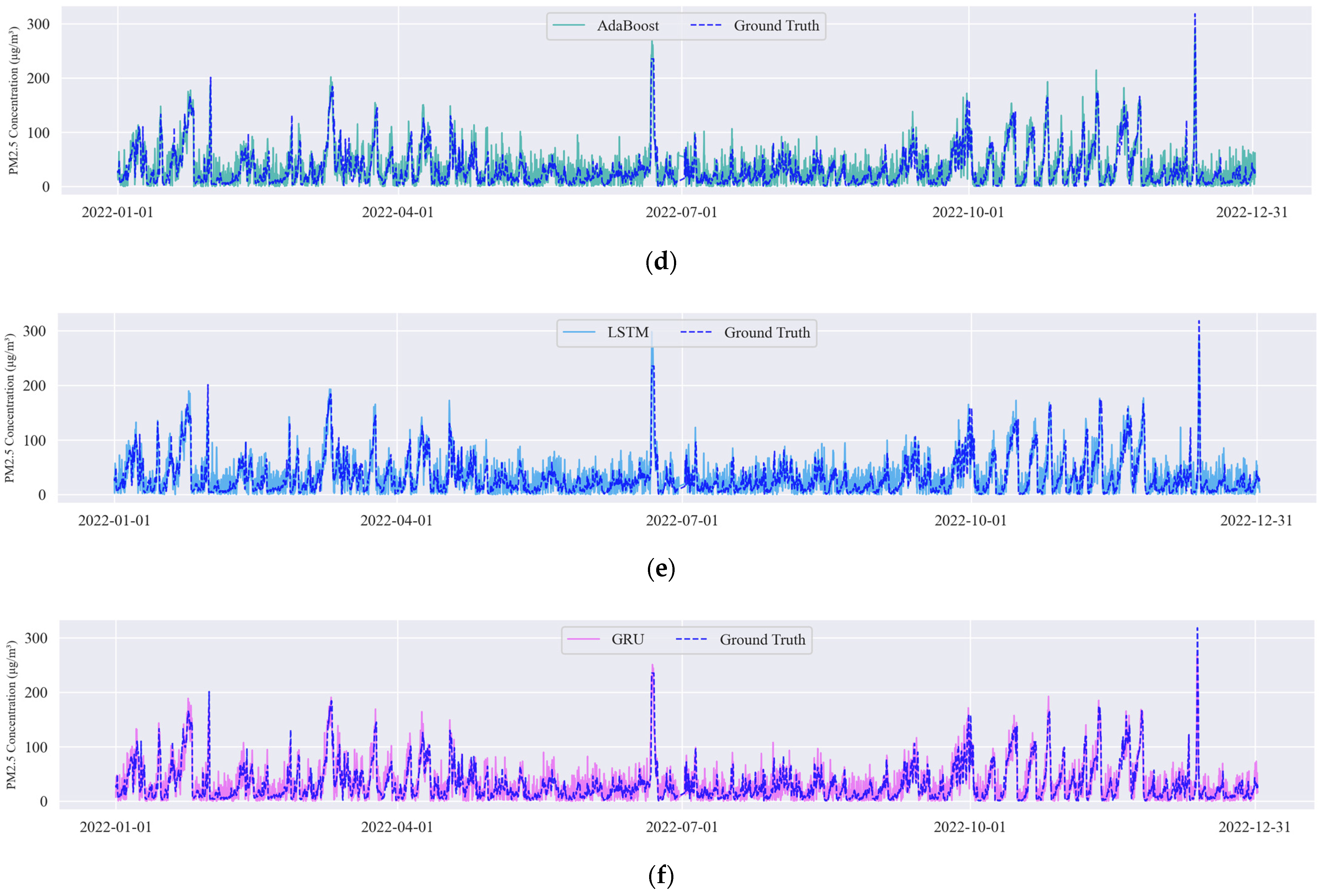
Figure 3 presents the time-series plots of PM2.5 predictions for each model throughout 2022 (Figure 3a–f). These graphs reveal that the MSAFormer model closely captures the true PM2.5 concentration trends, thereby evidencing its superior temporal modeling capability. Table 5 displays the RMSE, MAE, and R2 scores for all six models, from which it is apparent that the MSAFormer model exhibits the best predictive accuracy, marked by the lowest RMSE and MAE, as well as the highest R2 score.
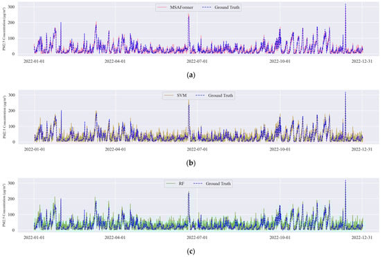

Figure 3.
Time-series plots of the PM2.5 predictions made by (a) MSAFormer, (b) SVM, (c) RF, (d) AdaBoost, (e) LSTM, and (f) GRU models for the year 2022.
Table 5.
Comparative performance of SVM, RF, AdaBoost, LSTM, GRU, and MSAFormer models in terms of RMSE, MAE, and R2 scores.
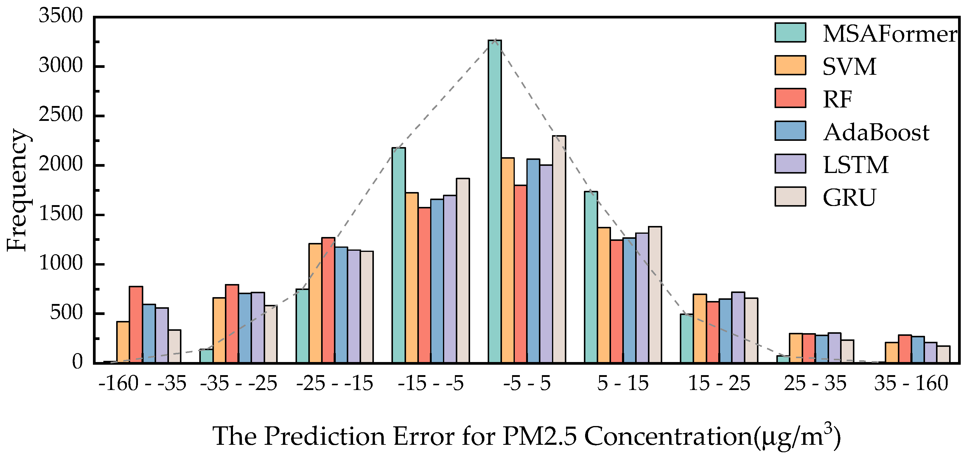
Lastly, the histogram of prediction errors (Figure 4) shows that the MSAFormer has a narrower error distribution, centralized around zero. This underlines its enhanced prediction performance as compared to the benchmark models, with smaller and fewer errors.
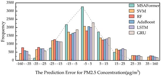
Figure 4.
Histogram of prediction errors for the six models: SVM, RF, AdaBoost, LSTM, GRU, and MSAFormer.
From these results, it can be concluded that the MSAFormer model presents significant improvements over traditional models in terms of predictive accuracy and the ability to effectively capture temporal dependencies in PM2.5 concentrations.
4.3. Sensitivity Analysis of the MSAFormer Model
This section conducts a sensitivity analysis to determine the influence of the Meteorological Sparse Autoencoding (MSA) module and the parameter, Sparse Autoencoder Coefficient (λ), on the overall performance of the proposed MSAFormer model. The first experiment was conducted without incorporating the MSA module into the MSAFormer model, meaning that meteorological factor data were not utilized for the PM2.5 concentration prediction. The second part of the analysis involved adjusting the Sparse Autoencoder Coefficient (λ), from 0.0 to 1.0 in increments of 0.1, to observe its impact on the model’s performance.
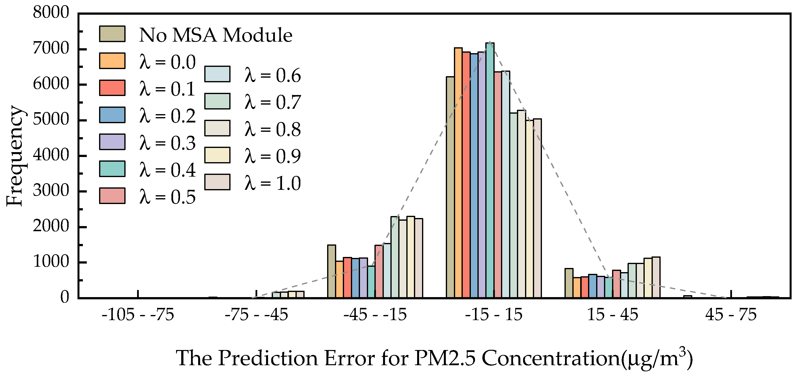
The experimental results are visually presented in Figure 5 and quantitatively summarized in Table 6. Figure 5 shows the error distribution of the MSAFormer model with varying λ values and the exclusion of the MSA module. An observable pattern from the graph is the decline in prediction error as λ increases, hitting a minimum at λ = 0.4, beyond which the error begins to rise, indicating an overfitting scenario.

Figure 5.
Error distribution of the MSAFormer model for different λ values and without the Meteorological Sparse Autoencoding module.
Table 6.
Comparative performance of the MSAFormer model for different λ values and without the Meteorological Sparse Autoencoding module, based on RMSE, MAE, and R2 scores.
The sensitivity analysis results shed light on the integral role of both the MSA module and the λ parameter in the MSAFormer model. Removing the MSA module leads to a substantial increase in error distribution, signifying the detrimental impact on the model’s performance. This indicates the importance of meteorological factors in achieving accurate PM2.5 concentration predictions, thereby validating the relevance and efficacy of the MSA module. As detailed in Table 6, different λ settings and the absence of the MSA module result in varying RMSE, MAE, and R2 scores for the MSAFormer model. An optimal λ value of 0.4 leads to the best model performance, with the lowest RMSE and MAE values and the highest R2 score. However, the absence of the MSA module does not lead to the worst performance, even though it leads to a considerable decrease in the accuracy of the predictions. The least satisfactory results are seen when λ is set to 1.0. These findings, in line with Figure 5, underscore the crucial role of the MSA module and the appropriate tuning of the λ parameter in maintaining the predictive accuracy of the MSAFormer model.
The observed outcomes reinforce the architectural rationale underpinning the MSAFormer model. The implementation of the MSA module, through a specialized sparse autoencoder, proficiently extracts meaningful features from meteorological variables sourced from nine distinct monitoring stations situated throughout Beijing. This advanced feature extraction significantly augments the model’s predictive proficiency for PM2.5 concentrations in the Haidian district. Moreover, these outcomes highlight the pivotal role played by the Sparse Autoencoder Coefficient (λ) in fine-tuning the balance between the sparsity of the feature representation and the generalization capability of the model. Notably, the model achieved optimal performance when the λ value was adjusted to 0.4. This finding suggests that a certain degree of sparsity within the autoencoder is beneficial in encapsulating critical meteorological features whilst concurrently circumventing overfitting, thus offering a compelling trade-off.
These findings unequivocally reaffirm the effectiveness and robustness of the MSAFormer model, underscoring its considerable potential for application in air quality prediction tasks, particularly in the realm of urban environmental management and public health.
5. Conclusions
In this study, we introduced MSAFormer, a transformative approach for PM2.5 concentration prediction, that offers significant improvement over conventional methodologies. The MSAFormer model creatively combines the advantages of the Transformer architecture with a Meteorological Sparse Autoencoding (MSA) module to tackle the inherent complexity of multi-station meteorological data. The MSA module effectively encapsulates the non-linear relationships in high-dimensional data by extracting salient features, overcoming the limitations of traditional methods. The Positional Embedding module further flattens the sparse-encoded features, enabling streamlined data processing in the subsequent Transformer module. In the final module, a self-attention mechanism is employed to capture temporal dependencies in the input data, thereby predicting future PM2.5 concentrations with increased precision.
Our experimental evaluation reveals that MSAFormer performs remarkably well in predicting PM2.5 concentrations in the Haidian district. In our study, we compared the MSAFormer model with traditional methods such as SVM, RF, AdaBoost, LSTM, and GRU. Specifically, the MSAFormer model demonstrates improvements in all the considered metrics: it lowers the RMSE by 6.935 to 11.888, reduces the MAE by 4.938 to 8.761, and enhances the R2 value by 0.146 to 0.266, compared to these traditional methods. Among these, the greatest improvement in R2 is observed over RF, with an increase of 29.621%. These quantitative advancements corroborate the efficacy of our model and the relevance of deep learning in environmental meteorological data analysis.
However, like all research, ours is not without limitations. The MSAFormer model relies heavily on the quality of input data. As such, data inconsistencies or inadequacies might affect the predictive capabilities of our model. Furthermore, while our model demonstrates superior performance in the Haidian district, the generalizability to other geographical locations and environmental contexts remains to be explored.
For future work, we recommend several avenues. First, the model’s robustness could be strengthened by incorporating additional sources of data and conducting multi-site evaluation tests. Second, the MSAFormer model could be further refined and generalized to predict other meteorological phenomena and pollutants, potentially contributing to a broader scope of environmental science. Finally, the implementation of the MSAFormer model in a real-world setting, such as urban air quality management systems, would provide valuable insights into its practical performance and utility.
Author Contributions
Conceptualization, H.W. and L.Z.; methodology, H.W.; software, H.W.; validation, H.W., L.Z. and R.W.; formal analysis, H.W.; investigation, H.W.; resources, H.W.; data curation, H.W.; writing—original draft preparation, H.W.; writing—review and editing, H.W.; visualization, H.W.; supervision, H.W.; project administration, H.W.; funding acquisition, L.Z. All authors have read and agreed to the published version of the manuscript.
Funding
This research was funded by the National Natural Science Foundation of China, grant number 41830108.
Institutional Review Board Statement
Not applicable.
Informed Consent Statement
Not applicable.
Data Availability Statement
The data presented in this study are available on request from the corresponding author.
Conflicts of Interest
The authors declare no conflict of interest.
References
- Patz, J.A. Public Health Risk Assessment Linked to Climatic and Ecological Change. Hum. Ecol. Risk Assess. Int. J. 2001, 7, 1317–1327. [Google Scholar] [CrossRef]
- Harlan, S.L.; Ruddell, D.M. Climate change and health in cities: Impacts of heat and air pollution and potential co-benefits from mitigation and adaptation. Curr. Opin. Environ. Sustain. 2011, 3, 126–134. [Google Scholar] [CrossRef]
- Singh, N.; Singh, S.; Mall, R.K. Urban ecology and human health: Implications of urban heat island, air pollution and climate change nexus. In Urban Ecology; Verma, P., Singh, P., Singh, R., Raghubanshi, A.S., Eds.; Elsevier: Amsterdam, The Netherlands, 2020; Chapter 17; pp. 317–334. [Google Scholar]
- Karimi, B.; Meyer, C.; Gilbert, D.; Bernard, N. Air pollution below WHO levels decreases by 40% the links of terrestrial microbial networks. Environ. Chem. Lett. 2016, 14, 467–475. [Google Scholar] [CrossRef]
- Zajchowski, C.A.B.; South, F.; Rose, J.; Crofford, E. The role of temperature and air quality in outdoor recreation behavior: A social-ecological systems approach. Geogr. Rev. 2022, 112, 512–531. [Google Scholar] [CrossRef]
- Wang, C.; Tu, Y.; Yu, Z.; Lu, R. PM2.5 and Cardiovascular Diseases in the Elderly: An Overview. Int. J. Environ. Res. Public Health 2015, 12, 8187–8197. [Google Scholar] [CrossRef] [PubMed]
- Liu, S.-T.; Liao, C.-Y.; Kuo, C.-Y.; Kuo, H.-W. The Effects of PM2.5 from Asian Dust Storms on Emergency Room Visits for Cardiovascular and Respiratory Diseases. Int. J. Environ. Res. Public Health 2017, 14, 428. [Google Scholar] [CrossRef] [PubMed]
- Luo, G.; Zhang, L.; Hu, X.; Qiu, R. Quantifying public health benefits of PM2.5 reduction and spatial distribution analysis in China. Sci. Total Environ. 2020, 719, 137445. [Google Scholar] [CrossRef]
- Al-Hemoud, A.; Gasana, J.; Al-Dabbous, A.; Alajeel, A.; Al-Shatti, A.; Behbehani, W.; Malak, M. Exposure levels of air pollution (PM2.5) and associated health risk in Kuwait. Environ. Res. 2019, 179, 108730. [Google Scholar] [CrossRef]
- McKeen, S.; Chung, S.H.; Wilczak, J.; Grell, G.; Djalalova, I.; Peckham, S.; Gong, W.; Bouchet, V.; Moffet, R.; Tang, Y.; et al. Evaluation of several PM2.5 forecast models using data collected during the ICARTT/NEAQS 2004 field study. J. Geophys. Res. Atmos. 2007, 112, 7608. [Google Scholar] [CrossRef]
- Mahajan, S.; Liu, H.M.; Tsai, T.C.; Chen, L.J. Improving the Accuracy and Efficiency of PM2.5 Forecast Service Using Cluster-Based Hybrid Neural Network Model. IEEE Access 2018, 6, 19193–19204. [Google Scholar] [CrossRef]
- Luo, C.H.; Yang, H.; Huang, L.P.; Mahajan, S.; Chen, L.J. A Fast PM2.5 Forecast Approach Based on Time-Series Data Analysis, Regression and Regularization. In Proceedings of the 2018 Conference on Technologies and Applications of Artificial Intelligence (TAAI), Taichung, Taiwan, 30 November–2 December 2018; pp. 78–81. [Google Scholar]
- Cho, S.; Park, H.; Son, J.; Chang, L. Development of the Global to Mesoscale Air Quality Forecast and Analysis System (GMAF) and Its Application to PM2.5 Forecast in Korea. Atmosphere 2021, 12, 411. [Google Scholar] [CrossRef]
- Hu, J.; Chen, J.; Ying, Q.; Zhang, H. One-year simulation of ozone and particulate matter in China using WRF/CMAQ modeling system. Atmos. Chem. Phys. 2016, 16, 10333–10350. [Google Scholar] [CrossRef]
- Mathur, R.; Xing, J.; Gilliam, R.; Sarwar, G.; Hogrefe, C.; Pleim, J.; Pouliot, G.; Roselle, S.; Spero, T.L.; Wong, D.C.; et al. Extending the Community Multiscale Air Quality (CMAQ) modeling system to hemispheric scales: Overview of process considerations and initial applications. Atmos. Chem. Phys. 2017, 17, 12449–12474. [Google Scholar] [CrossRef] [PubMed]
- Tuccella, P.; Curci, G.; Visconti, G.; Bessagnet, B.; Menut, L.; Park, R.J. Modeling of gas and aerosol with WRF/Chem over Europe: Evaluation and sensitivity study. J. Geophys. Res. Atmos. 2012, 117, 6302. [Google Scholar] [CrossRef]
- Sicard, P.; Crippa, P.; De Marco, A.; Castruccio, S.; Giani, P.; Cuesta, J.; Paoletti, E.; Feng, Z.; Anav, A. High spatial resolution WRF-Chem model over Asia: Physics and chemistry evaluation. Atmos. Environ. 2021, 244, 118004. [Google Scholar] [CrossRef]
- Wang, Q.; Zeng, Q.; Tao, J.; Sun, L.; Zhang, L.; Gu, T.; Wang, Z.; Chen, L. Estimating PM2.5 Concentrations Based on MODIS AOD and NAQPMS Data over Beijing–Tianjin–Hebei. Sensors 2019, 19, 1207. [Google Scholar] [CrossRef] [PubMed]
- Zeng, Q.; Zhu, H.; Gao, Y.; Xie, T.; Liu, S.; Chen, L. Estimating Full-Coverage PM2.5 Concentrations Based on Himawari-8 and NAQPMS Data over Sichuan-Chongqing. Appl. Sci. 2022, 12, 7065. [Google Scholar] [CrossRef]
- Mariano, P.; Almeida, S.M.; Santana, P. On the automated learning of air pollution prediction models from data collected by mobile sensor networks. Energy Sources Part A Recovery Util. Environ. Eff. 2021, 2021, 1–17. [Google Scholar] [CrossRef]
- Wu, Z.; Liu, N.; Li, G.; Liu, X.; Wang, Y.; Zhang, L. Learning Adaptive Probabilistic Models for Uncertainty-Aware Air Pollution Prediction. IEEE Access 2023, 11, 24971–24985. [Google Scholar] [CrossRef]
- Barnard, J.C.; Fast, J.D.; Paredes-Miranda, G.; Arnott, W.P.; Laskin, A. Technical Note: Evaluation of the WRF-Chem “Aerosol Chemical to Aerosol Optical Properties” Module using data from the MILAGRO campaign. Atmos. Chem. Phys. 2010, 10, 7325–7340. [Google Scholar] [CrossRef]
- Jiang, F.; Liu, Q.; Huang, X.; Wang, T.; Zhuang, B.; Xie, M. Regional modeling of secondary organic aerosol over China using WRF/Chem. J. Aerosol Sci. 2012, 43, 57–73. [Google Scholar] [CrossRef]
- Zhang, Y.; Pan, Y.; Wang, K.; Fast, J.D.; Grell, G.A. WRF/Chem-MADRID: Incorporation of an aerosol module into WRF/Chem and its initial application to the TexAQS2000 episode. J. Geophys. Res. Atmos. 2010, 115, 3443. [Google Scholar] [CrossRef]
- Ge, B.Z.; Wang, Z.F.; Xu, X.B.; Wu, J.B.; Yu, X.L.; Li, J. Wet deposition of acidifying substances in different regions of China and the rest of East Asia: Modeling with updated NAQPMS. Environ. Pollut. 2014, 187, 10–21. [Google Scholar] [CrossRef] [PubMed]
- Tie, X.; Brasseur, G.; Ying, Z. Impact of model resolution on chemical ozone formation in Mexico City: Application of the WRF-Chem model. Atmos. Chem. Phys. 2010, 10, 8983–8995. [Google Scholar] [CrossRef]
- Tan, J.; Liu, H.; Li, Y.; Yin, S.; Yu, C. A new ensemble spatio-temporal PM2.5 prediction method based on graph attention recursive networks and reinforcement learning. Chaos Solitons Fractals 2022, 162, 112405. [Google Scholar] [CrossRef]
- Masood, A.; Ahmad, K. Data-driven predictive modeling of PM2.5 concentrations using machine learning and deep learning techniques: A case study of Delhi, India. Environ. Monit. Assess. 2022, 195, 60. [Google Scholar] [CrossRef] [PubMed]
- Xu, Y.; Zhao, X.; Chen, Y. Short-term PM2.5 prediction based on a data-driven heuristic approach. In Proceedings of the 2022 3rd International Conference on Electronic Communication and Artificial Intelligence (IWECAI), Zhuhai, China, 14–16 January 2022; pp. 534–539. [Google Scholar]
- Lai, X.; Li, H.; Pan, Y. A combined model based on feature selection and support vector machine for PM2.5 prediction. J. Intell. Fuzzy Syst. 2021, 40, 10099–10113. [Google Scholar] [CrossRef]
- Mogollón-Sotelo, C.; Casallas, A.; Vidal, S.; Celis, N.; Ferro, C.; Belalcazar, L. A support vector machine model to forecast ground-level PM2.5 in a highly populated city with a complex terrain. Air Qual. Atmos. Health 2021, 14, 399–409. [Google Scholar] [CrossRef]
- Babu, S.; Thomas, B. A survey on air pollutant PM2.5 prediction using random forest model. Environ. Health Eng. Manag. J. 2023, 10, 157–163. [Google Scholar] [CrossRef]
- Wang, Y.; Du, Y.; Fang, J.; Dong, X.; Wang, Q.; Ban, J.; Sun, Q.; Ma, R.; Zhang, W.; He, M.Z.; et al. A Random Forest Model for Daily PM2.5 Personal Exposure Assessment for a Chinese Cohort. Environ. Sci. Technol. Lett. 2022, 9, 466–472. [Google Scholar] [CrossRef]
- Liu, H.; Jin, K.; Duan, Z. Air PM2.5 concentration multi-step forecasting using a new hybrid modeling method: Comparing cases for four cities in China. Atmos. Pollut. Res. 2019, 10, 1588–1600. [Google Scholar] [CrossRef]
- Kim, H.S.; Han, K.M.; Yu, J.; Kim, J.; Kim, K.; Kim, H. Development of a CNN+LSTM Hybrid Neural Network for Daily PM2.5 Prediction. Atmosphere 2022, 13, 2124. [Google Scholar] [CrossRef]
- Dong, J.; Liu, P.; Song, H.; Yang, D.; Yang, J.; Song, G.; Miao, C.; Zhang, J.; Zhang, L. Effects of anthropogenic precursor emissions and meteorological conditions on PM2.5 concentrations over the “2+26” cities of northern China. Environ. Pollut. 2022, 315, 120392. [Google Scholar] [CrossRef]
- Zhang, J.; Liu, P.; Song, H.; Miao, C.; Yang, J.; Zhang, L.; Dong, J.; Liu, Y.; Zhang, Y.; Li, B. Multi-Scale Effects of Meteorological Conditions and Anthropogenic Emissions on PM2.5 Concentrations over Major Cities of the Yellow River Basin. Int. J. Environ. Res. Public Health 2022, 19, 15060. [Google Scholar] [CrossRef]
- Xing, Q.; Sun, M. Characteristics of PM2.5 and PM10 Spatio-Temporal Distribution and Influencing Meteorological Conditions in Beijing. Atmosphere 2022, 13, 1120. [Google Scholar] [CrossRef]
- Górka, M.; Trzyna, A.; Lewandowska, A.; Drzeniecka-Osiadacz, A.; Miazga, B.; Rybak, J.; Widory, D. The impact of seasonality and meteorological conditions on PM2.5 carbonaceous fractions coupled with carbon isotope analysis: Advantages, weaknesses and interpretation pitfalls. Atmos. Res. 2023, 290, 106800. [Google Scholar] [CrossRef]
- Niu, M.; Zhang, Y.; Ren, Z. Deep Learning-Based PM2.5 Long Time-Series Prediction by Fusing Multisource Data—A Case Study of Beijing. Atmosphere 2023, 14, 340. [Google Scholar] [CrossRef]
- Kim, B.-Y.; Lim, Y.-K.; Cha, J.W. Short-term prediction of particulate matter (PM10 and PM2.5) in Seoul, South Korea using tree-based machine learning algorithms. Atmos. Pollut. Res. 2022, 13, 101547. [Google Scholar] [CrossRef]
- Zheng, Q.; Tian, X.; Yu, Z.; Jiang, N.; Elhanashi, A.; Saponara, S.; Yu, R. Application of wavelet-packet transform driven deep learning method in PM2.5 concentration prediction: A case study of Qingdao, China. Sustain. Cities Soc. 2023, 92, 104486. [Google Scholar] [CrossRef]
- Yan, L.; Zhou, M.; Wu, Y.; Yan, L. Long Short Term Memory Model for Analysis and Forecast of PM2.5. In Proceedings of the Cloud Computing and Security, Haikou, China, 8–10 June 2018; pp. 623–634. [Google Scholar]
- Moursi, A.S.A.; El-Fishawy, N.; Djahel, S.; Shouman, M.A. Enhancing PM2.5 Prediction Using NARX-Based Combined CNN and LSTM Hybrid Model. Sensors 2022, 22, 4418. [Google Scholar] [CrossRef]
- Liu, X.; Li, W. MGC-LSTM: A deep learning model based on graph convolution of multiple graphs for PM2.5 prediction. Int. J. Environ. Sci. Technol. 2022, 20, 10297–10312. [Google Scholar] [CrossRef]
- Huang, G.; Li, X.; Zhang, B.; Ren, J. PM2.5 concentration forecasting at surface monitoring sites using GRU neural network based on empirical mode decomposition. Sci. Total Environ. 2021, 768, 144516. [Google Scholar] [CrossRef] [PubMed]
- Faraji, M.; Nadi, S.; Ghaffarpasand, O.; Homayoni, S.; Downey, K. An integrated 3D CNN-GRU deep learning method for short-term prediction of PM2.5 concentration in urban environment. Sci. Total Environ. 2022, 834, 155324. [Google Scholar] [CrossRef] [PubMed]
- Karimian, H.; Li, Y.; Chen, Y.; Wang, Z. Evaluation of different machine learning approaches and aerosol optical depth in PM2.5 prediction. Environ. Res. 2023, 216, 114465. [Google Scholar] [CrossRef] [PubMed]
- Gokul, P.R.; Mathew, A.; Bhosale, A.; Nair, A.T. Spatio-temporal air quality analysis and PM2.5 prediction over Hyderabad City, India using artificial intelligence techniques. Ecol. Inform. 2023, 76, 102067. [Google Scholar] [CrossRef]
- Zhou, H.; Zhang, F.; Du, Z.; Liu, R. A theory-guided graph networks based PM2.5 forecasting method. Environ. Pollut. 2022, 293, 118569. [Google Scholar] [CrossRef] [PubMed]
- Zhang, Q.; Yang, G.; Yuan, E. PM2.5 Spatial-Temporal Long Series Forecasting Based on Deep Learning and EMD. In Proceedings of the Knowledge and Systems Sciences, Singapore, 11–12 June 2022; pp. 3–19. [Google Scholar]
- Yang, H.C.; Yang, M.C.; Wong, G.W.; Chen, M.C. Extreme Event Discovery With Self-Attention for PM2.5 Anomaly Prediction. IEEE Intell. Syst. 2023, 38, 36–45. [Google Scholar] [CrossRef]
- Zhou, L.; Wu, T.; Pu, L.; Meadows, M.; Jiang, G.; Zhang, J.; Xie, X. Spatially heterogeneous relationships of PM2.5 concentrations with natural and land use factors in the Niger River Watershed, West Africa. J. Clean. Prod. 2023, 394, 136406. [Google Scholar] [CrossRef]
- Li, J.; Dai, Y.; Zhu, Y.; Tang, X.; Wang, S.; Xing, J.; Zhao, B.; Fan, S.; Long, S.; Fang, T. Improvements of response surface modeling with self-adaptive machine learning method for PM2.5 and O3 predictions. J. Environ. Manag. 2022, 303, 114210. [Google Scholar] [CrossRef]
- Vaswani, A.; Shazeer, N.; Parmar, N.; Uszkoreit, J.; Jones, L.; Gomez, A.N.; Kaiser, Ł.; Polosukhin, I. Attention is all you need. Adv. Neural Inf. Process. Syst. 2017, 30. [Google Scholar] [CrossRef]
- Castangia, M.; Grajales, L.M.M.; Aliberti, A.; Rossi, C.; Macii, A.; Macii, E.; Patti, E. Transformer neural networks for interpretable flood forecasting. Environ. Model. Softw. 2023, 160, 105581. [Google Scholar] [CrossRef]
- Kumbalaparambi, T.S.; Menon, R.; Radhakrishnan, V.P.; Nair, V.P. Assessment of urban air quality from Twitter communication using self-attention network and a multilayer classification model. Environ. Sci. Pollut. Res. 2023, 30, 10414–10425. [Google Scholar] [CrossRef]
- Han, X.-H.; Chen, Y.-W. Residual Sparse Autoencoders for Unsupervised Feature Learning and Its Application to HEp-2 Cell Staining Pattern Recognition. In Deep Learning in Healthcare: Paradigms and Applications; Chen, Y.-W., Jain, L.C., Eds.; Springer International Publishing: Cham, Switzerland, 2020; pp. 181–199. [Google Scholar]
Disclaimer/Publisher’s Note: The statements, opinions and data contained in all publications are solely those of the individual author(s) and contributor(s) and not of MDPI and/or the editor(s). MDPI and/or the editor(s) disclaim responsibility for any injury to people or property resulting from any ideas, methods, instructions or products referred to in the content. |
© 2023 by the authors. Licensee MDPI, Basel, Switzerland. This article is an open access article distributed under the terms and conditions of the Creative Commons Attribution (CC BY) license (https://creativecommons.org/licenses/by/4.0/).